Page 1 INSTRUCTION MANUAL MODEL ZA3000 SERIES POLARIZED ZEEMAN ATOMIC ABSORPTION SPECTROPHOTOMETER (OPERATION MANUAL : FLAME ANALYSIS) Hitachi High-Technologies Corporation 24-14, Nishi-Shimbashi 1-chome, Minato-ku, Tokyo, Japan 2nd Edition, December 2012 Copyright C Hitachi High-Technologies Corporation 2012. 1st Edition, 2012 All rights reserved. Printed in Japan.
Page 2 NOTICE: Information contained in this document is subject to change without notice for improvement. This manual is copyrighted by Hitachi High-Technologies Corporation with all rights reserved. No part of this manual may be reproduced, transmitted or disclosed to a third party in any form or by any means without the express written permission of Hitachi High-Technologies Corporation.
Page 3: Preface
PREFACE We are grateful for your purchase of Hitachi ZA3000 Series Polarized Zeeman Atomic Absorption Spectrophotometer. The ZA3000 series atomic absorption spectrophotometer is an instrument designed for elemental analysis. This instrument is intended for use by persons having a basic knowledge of chemical analysis. Analysis with this...
Page 4: Safety Summary
SAFETY SUMMARY Definition of Alert Symbol and Signal Word Before using the ZA3000 Series Polarized Zeeman Atomic Absorption Spectrophotometer, carefully read the safety instructions given below. The hazard warnings which appear on the warning labels on the product or in the manual have one of the following alert headings...
Page 5: General Safety Guidelines
SAFETY SUMMARY General Safety Guidelines Precautions before Use  Before using the instrument, be sure to read this manual carefully until you fully understand its contents.  Keep this manual in a safety place nearby so that it can be referred to whenever needed.
Page 6 SAFETY SUMMARY General Safety Guidelines (Continued)  Keep in mind that the hazard warnings in this manual and on the instrument cannot cover every possible case, as it is impossible to predict and evaluate all circumstances beforehand. Therefore, just following the given directions may be inadequate for operation.
Page 7 SAFETY SUMMARY General Safety Guidelines (Continued) Precautions on Installation, Maintenance and Relocation  The customer shall not attempt initial installation (upon delivery) of the instrument. For safe and exact use of the instrument, service personnel trained and approved by us will carry out the installation. ...
Page 8: Warning Indications In This Manual
SAFETY SUMMARY Warning Indications in this Manual Warning indications described in this manual and their locations in it are listed below. List of DANGER Indications  Malfunction of Pacemaker! There is a danger of faulty operation of a pacemaker due to the strong magnetic field produced.
Page 9: List Of Warning Indications
SAFETY SUMMARY List of WARNING Indications  Beware of High Voltage! There is a danger of electric shock due to high voltage of about 400 V. Touching the socket of the hollow cathode lamp could result in fatal or serious injury. Before replacing the lamp, be sure to turn OFF the lamp current (click the lamp OFF button).
Page 10: Explosion Due To Perchloric Acid
SAFETY SUMMARY List of WARNING Indications (Continued)  Explosion due to Perchloric Acid! If metals (copper, silver and mercury) that form metal acetylide and perchloric acid are contained in a sample when using a high-temperature burner, they react in the flame chamber and may result into explosions with loud noise due to backfiring.
Page 11: List Of Caution Indications
SAFETY SUMMARY List of CAUTION Indications  Strong Magnetic Fields! Be careful not to let your hand get attracted to the magnet. Do not bring metal objects including iron, such as a screwdriver, near the magnet. (Sections 3 and 5 in this manual) ...
Page 12: List Of Caution Indications
SAFETY SUMMARY List of CAUTION Indications  Malfunction by Wrong Gas Type! Hydrogen flame cannot be used by this instrument. Never connect hydrogen gas to this instrument. (Section 1 in this manual)  Deterioration of Burner Chamber by Chemicals! A strong acid other than hydrochloric acid or hydrofluoric acid may damage the burner chamber.
Page 13: Table Of Contents
CONTENTS PREFACE ABOUT THIS MANUAL SAFETY SUMMARY .................. SAFETY-1 Definition of Alert Symbol and Signal Word .. SAFETY-1 General Safety Guidelines ......SAFETY-2 Warning Indications in this Manual ....SAFETY-5 List of DANGER Indications ......SAFETY-5 Malfunction of Pacemaker! ........ SAFETY-5 List of WARNING Indications ......
Page 14 Fundamental Operation of Software Windows ... 2-5 2.3.1 Clicking and Double-clicking ....... 2-5 2.3.2 Names and Functions of Window Elements ............ 2-5 2.3.3 How to Input Measurement Conditions ..2-7 2.3.4 Opening Files ..........2-10 2.3.5 Saving Files ..........2-11 2.3.6 Asking for Help ...........
Page 15 3.12 Changing the Display of a Working Curve Graph ......... 3-45 3.13 Termination of Measurement ........ 3-46 CHECKING THE RESULT ..................4-1 Data Table .............. 4-2 4.1.1 Error Marks..........4-4 4.1.2 Correction of Operator, Analysis Name, and Comment ....4-5 Profile Graph ............
Page 16 5.5.1 Insertion of Samples ........5-14 5.5.2 Remeasurement ......... 5-15 Auto-Start ............... 5-16 Auto-Flame Off ............5-18 Emission Measurement ......... 5-19 Using Monitor Measuring Function ...... 5-22 5.10 Setting Automatic Start ......... 5-25 5.11 Power/Water Saving by Eco Mode ....... 5-27 5.11.1 Setting Eco Mode ........
Page 17 8.3.5 Checking and Saving the Diagnostic Results ............8-9 8.3.6 Output of Diagnostic Results ...... 8-11 TROUBLESHOOTING .................... 9-1 INDEX ........................INDEX-1 - v -...
Page 18: Start Up
1. START UP The procedure below should be implemented prior to supplying power to the spectrometer. 1.1 Check of Instrument On the main unit of atomic absorption spectrophotometer, perform the following checks. Is each unit of the instrument (main unit, PC, and optional accessories such as autosampler) connected properly? For cable connection, coolant piping and gas piping, refer to the maintenance edition.
Page 19: Mounting Of Hollow Cathode Lamps
1.2 Mounting of Hollow Cathode Lamps CAUTION Do Not Touch Hot Parts! There is a danger of burns upon touching heated parts. Especially the burner remains hot for a while even after extinguishing the flame. Before exchanging the burner, wait at least 10 minutes for it to cool down. CAUTION Malfunction by Wrong Gas Type! Hydrogen flame cannot be used by this instrument.
Page 20 If the lamp socket is not secured properly, it may snag on another lamp and cause motor malfunction or break a lamp. The lamp made by Hitachi High-Technologies should use HLA-4 type. Since, as for the old products (HLA-3 type etc.), the lamp code may be caught it cannot be used.
Page 21: Supply Of Gases
1.3 Supply of Gases 1.3 Supply of Gases Prepare the fuel and auxiliary gases in accordance with the atomizer to be used. Atomizer Combination of Fuel and Auxiliary Gases Standard burner Air-acetylene, air High-temperature Nitrous oxide-acetylene, air-acetylene, air burner Hg cell ...
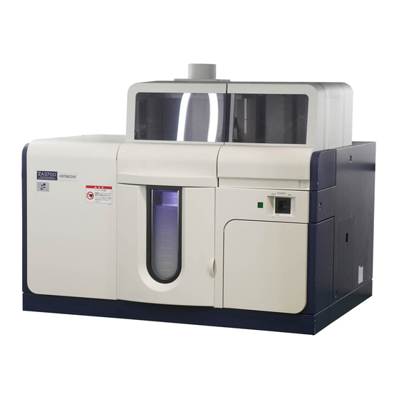
Page 22: Power-On
1.4 Power-on Turn ON the respective power switches of the PC and peripheral devices such as printer that are connected to the instrument. Turn ON the power switch (Fig. 1-2) on the front right of the atomic absorption spectrophotometer. Then start up the PC. Power switch Fig.
Page 23: Power-On Of Exhaust Duct
1.5 Power-on of Exhaust Duct 1.5 Power-on of Exhaust Duct Turn on power supply of the exhaust duct line to rotate the fan. Use the exhaust duct airflow in the range from 600 to 1200 m near the frame opening at the upper part of the main body. When there is a large airflow, conduct airflow adjustment using dampers.
Page 24 Check of instrument, and preparation of hollow cathode lamps and gas Power-on of PC, spectrophotometer main unit and duct Startup of AAS program Setting of measurement conditions Execution of Set Conditions Supply of gas and cooling water Turning on flame Aspiration of purified water for 5 minutes Execution of auto zero Measurement of standard sample...
Page 25: Startup Of Software
2. STARTUP OF SOFTWARE 2.1 Startup of Atomic Absorption Spectrophotometer Program Turn on power to the spectrophotometer main unit, wait at least 15 seconds, and then double-click the shortcut icon “Zeeman AAS” (Fig. 2-1) on the PC screen. Fig. 2-1 Shortcut Icon of Zeeman AAS The initialization window appears, and the atomic absorption spectrophotometer program is started.
Page 26: Setting The Instrument Online
2.2 Setting the Instrument Online 2.2 Setting the Instrument Online The following two states are possible for the atomic absorption spectrophotometer program.  Online status: Measurement can be performed through control of the spectrophotometer main unit.  Offline status: Data processing can be executed on the PC side alone without controlling the spectrophotometer main unit (status in which online mode is inactive).
Page 27: At Startup] Is Selected
2.2.1 Fig. 2-4 Check of Progress of Online Processing  In the case where [Set Conditions at Startup] is specified, condition setting will be executed under the specified measurement conditions. Make sure of no water leak from the cooling water flow path and click OK if no problem is found.
Page 28: When
2.2 Setting the Instrument Online On completion of program start, the Method window shown 2.2.2 When [Communicate in Fig. 2-3 appears. with Instrument For setting the online status, click [On-line] in the [Tools] at Startup] is Not menu in the menu bar (see Fig. 2-6). Selected The progress of the initialization can be checked via the status of the time bar shown during the online mode (Fig.
Page 29: Fundamental Operation Of Software Windows
2.3.1 2.3 Fundamental Operation of Software Windows Explained next are the fundamentals of window operation with the atomic absorption spectrophotometer software. 2.3.1 Clicking and “Clicking” and “double-clicking” are the mouse operations Double-clicking necessary for operating the atomic absorption spectrophotometer.  Clicking : Press and release the left mouse button quickly.
Page 30 2.3 Fundamental Operation of Software Windows Menu Bar Contains [File], [View] and other menu items which are arranged horizontally. The items on the menu bar vary with the window. There are two methods of selecting a menu or command.  Move the mouse pointer to a menu item and click it. ...
Page 31: How To Input Measurement Conditions
2.3.3 Toolbox Contains a number of large buttons arranged vertically on the left edge of the screen. Buttons that are frequently used for start of measurement, window selection, etc. are displayed here. As with the toolbar buttons, the name of each button can be checked by using the mouse.
Page 32 2.3 Fundamental Operation of Software Windows Putting Check Mark in Check Box To insert a checkmark, click with the cursor in a check box . As shown in Fig. 2-10, a check mark is put in the box to indicate the selected status. When clicking the check box again, the check mark disappears to indicate the unselected status.
Page 33 2.3.3 (5) Input of Character String In the display as shown in Fig. 2-13, you can input a character string directly after clicking inside text box. Move the mouse pointer onto the input column, and the maximum number of characters will be displayed in a tooltip frame.
Page 34: Opening Files
2.3 Fundamental Operation of Software Windows A method or data file can be opened in the following procedure. 2.3.4 Opening Files Click the [Open] button on the toolbar or click [Open Method File] or [Open Data File] in the [File] menu. The file opening dialog box as shown in Fig.
Page 35: Saving Files
2.3.5  When clicking the button, a new folder can be created.  When clicking the button, a new file display format can be selected. The files saved in the specified folder are displayed in the column under [Look in]. In this case, only the files of the type specified in [Files of type] are displayed.
Page 36 2.3 Fundamental Operation of Software Windows the method) and a data file has the name Resultyyyy_mmdd_hhmm_ss.adf (yyyy mm dd hh mm ss denotes the date and time point of measurement end). The default names may be used as they are. Fig.
Page 37: Asking For Help
2.3.6 The Help feature is useful when you don’t know how to operate 2.3.6 Asking for Help or you want a detailed explanation. Calling Help for Window Click the [Help] button in the tool bar in the [Method] window to display the help for the presently open window. Clicking a description with a green underscore displays the help for that description (Fig.
Page 38 2.3 Fundamental Operation of Software Windows Clicking the [Help] button (Fig. 2-17) can display the help window [Fig. 2-18] in the dialog box opened by the operation in the [Method] window. Fig. 2-17 Save Analysis Results as Dialog Box Fig. 2-18 Help Window Checking with Contents Open the [Help] menu and select the [Index] command in the menu bar.
Page 39 2.3.6 Checking with Keyword Input the characters to be searched in the keyword input box on the Help window, and the searched keywords will be displayed. Select the objective item and click the [Display] button. The relevant help will be displayed. Fig.
Page 40: Measurement With Conditions Input
3. MEASUREMENT WITH CONDITIONS INPUT The input of measurement conditions and measurement procedure are described here using quantitative measurement by an analysis of working curve method as an example. 3.1 Generation of Measurement Conditions The procedure for creating new measurement conditions is described next.
Page 41: Displaying The Method Window
3.1 Generation of Measurement Conditions When the Method window is not yet opened, click the [Method] 3.1.1 Displaying the button (<13> in Fig. 3-1) on the toolbox and the Method window Method Window will appear. Click the [Measurement Mode] button (<1> in Fig. 3-1) to open 3.1.2 Setting the measurement mode window.
Page 42 3.1.3 Click the elements to be analyzed in order on the Periodic Table (<1> in Fig. 3-2). The selected elements will change to green and will be added to the [Element-Order] table (<2> in Fig. 3-2). A maximum of 8 lamps can be set in the instrument, and when using multi-element lamps, up to 12 elements can be set.
Page 43: Instrument Setup
3.1 Generation of Measurement Conditions Click the [Instrument Setup] button (<3> in Fig. 3-3) and the 3.1.4 Instrument Setup Instrument Setup window will open. <1> Fig. 3-3 Instrument Setup Window The tab for the element selected in the Element window will be displayed.
Page 44 3.1.4 Emission intensity: Used in emission mode measurement.  Calculation Mode Integral is normally used, and need not be changed. The other modes are mainly used in graphite furnace analysis. Integral : Peak area is converted to area per second. This is mainly used in flame analysis.
Page 45 3.1 Generation of Measurement Conditions The analytical wavelengths can be checked via [Tools]- [Analytical Information] on the Method window. Input range for wavelength is from 190.0 to 900.0 nm. NOTES: 1. The Sensitivity Ratio is the rough value (Literature value) when the highest sensitivity wavelength is assumed to be “1”.
Page 46 3.1.4  Time Constant The time constant expresses the degree of signal smoothing. A larger time constant provides a reduced noise but a damped rise of the signal. A value of 1.0 second is normally used for flame analysis, and need not be changed. When there is much noise in the signal, a value of 2.0 may be better.
Page 47: Setting Analytical Conditions
3.1 Generation of Measurement Conditions 3.1.5 Setting Analytical Click the [Analytical Condition] button (<4> in Fig. 3-5) and Conditions the Analytical Condition window will appear. Fig. 3-5 Analytical Condition Window Set the following items.  Atomizer Normally the optimum device for the set element is selected by default, and need not be changed.
Page 48 3.1.5  Fuel Flow Input ranges are as follows. Air-C : 1.0 to 4.5 L/min (when the standard burner is used) : 5.0 to 8.0 L/min (when the high- temperature burner is used) Normally a flow rate (corresponding to the atomizer and type of flame) that is suitable for the set element is selected by default, and need not be changed for the Standard Burner.
Page 49 3.1 Generation of Measurement Conditions  Measurement Time Obtain the absorbance data for the time set from the start of measurement and calculate the level of absorbance. This is normally set at about 5 seconds. Input range is from 0.5 to 20 seconds. ...
Page 50: Setting Standards Table
3.1.6 Click the [Standards Table] button (<5> in Fig. 3-1) to open 3.1.6 Setting Standards Table the Standards Table window (Fig. 3-6). <1> Fig. 3-6 Standards Table Window 3 - 11...
Page 51 3.1 Generation of Measurement Conditions Set the following items.  Determination Mode [Absorbance] is used to measure the absorbance of a solution but does not quantify the solution. [Working Curve] is used to perform quantitative analysis of a sample in which coexisting materials contained in an unknown sample do not affect the atomization of the element.
Page 52 3.1.6  No. of STDs Specify the number of standard solutions (usually 3 to 5). Input range is from 2 to 10. From about 3 to 5 standards is normally sufficient. Input range is from 1 to 20. If the order is linear and the number of STDs is 2, the correlation coefficient is necessarily 1.
Page 53 3.1 Generation of Measurement Conditions decimal digits, a value obtained by rounding off the digits below the specified number is used as the standard sample concentration. Also, if the effective number of digits including decimal digits exceeds six, the number of decimal digits should be reduced so the effective number will be six.
Page 54: Setting Sample Table
3.1.7  UNK Unit Input the unit of unknown sample concentration. If the dilution factor is entered, the unit may be different from that for the STD sample. Carefully check before entering the factor. Input will be accepted in up to 6 characters. Even if this input is omitted, measurement can be performed.
Page 55 3.1 Generation of Measurement Conditions NOTE: All of the data on [ID], [Sample Name], [Weight], [Solvent], [Dil. Factor] and [Factor] of the entered sample table is reset.  [Change] button Used to change the [No. of UNK] of [Number of Samples].
Page 56 3.1.7 b. When the number of samples in sample table equals the entered [No. of UNK]: Content of the sample table will not be changed. c. When the entered [No. of UNK] is smaller than the number of samples in sample table: Example of execution;...
Page 57 3.1 Generation of Measurement Conditions UNK] button. Fig. 3-12 Insert of UNK Sample (1) The UNK sample is inserted in the sample table. The ID of the inserted sample becomes [4]. Fig. 3-13 Insert of UNK Sample (2) NOTE: The ID of the inserted UNK sample must change so as not to overlap with the ID of the existing UNK sample.
Page 58 3.1.7 Fig. 3-15 Delete of UNK Sample (2) Entry of Sample Names Select the [Sample Name] part of the table and enter sample names. Input range is up to 24 characters. Measurement can be made even if sample names are omitted.
Page 59 3.1 Generation of Measurement Conditions b. Click the object rows in sequence with the mouse while holding down the Ctrl key, and only those rows will be selected as indicated in Fig. 3-17. Fig. 3-17 Row Selection Method (2) (with automatic numbering) For setting the standard sample name, click the [STD Sample Name] button to open the entry window, and enter sample names the same as with unknown samples.
Page 60 3.1.7 Input for Concentration Correction When a sample has been diluted through pretreatment, the original concentration can be calculated. For this purpose, enter numerics into the [Weight], [Solvent], [Dil. Factor] and [Factor] columns. When calculation for concentration correction is not particularly required, then changes need not be made (“1”...
Page 61: Setting Qc Conditions
3.1 Generation of Measurement Conditions Setting of Measurement Object Click the [Measure Object] tab (<1> in Fig. 3-19) to display the Measure Object window. <1> Fig. 3-19 Measure Object Window The sample to be measured is indicated by , and specification can be made per element.
Page 62: Setting Report Format
3.1.9 Click the [Report Format] button (<9> in Fig. 3-1) to display the 3.1.9 Setting Report Report Format dialog. Auto-printing at the end of measurement Format and the items to be printed can be selected here. When auto-printing is not specified, printing can be made upon selecting the desired items at the end of measurement.
Page 63 3.1 Generation of Measurement Conditions Fig. 3-20 Parameter List Window (for each element) Fig. 3-21 Parameter List Window (Conditions common to all elements) The setting of method is thus completed. 3 - 24...
Page 64: Verification Of Measurement Condition
3.2 Verification of Measurement Condition The set or updated contents in the Method window remain in the editing status until you press the Verify button. Only after clicking the Verify button, does the relevant measurement condition become valid. Click the [Verify] button (<14> in Fig. 3-1). A dialog box for saving of analytical conditions will appear.
Page 65: Monitoring Of Measurement Process
3.3 Monitoring of Measurement Process 3.3 Monitoring of Measurement Process The progress of measurement can be checked on the Monitor window. This window consists of 5 sections as shown in Fig. 3-23. The size of 4 sections, excluding the Instrument Monitor Bar, can be changed by dragging them with the mouse cursor aligned with the boundary.
Page 66 Profile Graph The profile of atomization signals is displayed. This graph is a simple monitor display and its data is not saved. Therefore, if you change display mode, the past profile will be erased. Display of all measured data is allowed on the Data Process window after measurement.
Page 67 3.3 Monitoring of Measurement Process Instrument Monitor Bar Analyte element, message and analysis mode are displayed. In addition, the following items are displayed.  ABS Absorbance signal (background corrected) is displayed in real time.  REF Reference signal (background absorption) is displayed in real time.
Page 68 Indicates the status of the drain trap sensor. A red indication is provided when the water volume is low or the switch of the drain lid is not fully inserted. These indicate the status and present flow rate of fuel gas and oxidant gas.
Page 69: Wavelength Adjustment
3.4 Wavelength Adjustment 3.4 Wavelength Adjustment Before start of measurement, turn on the hollow cathode lamp and carry out wavelength adjustment. Even if this procedure is skipped, it will be automatically implemented at start of measurement. However, stabilization of lamp energy takes about 5 to 15 minutes, so this procedure should be implemented here.
Page 70 On the menu bar, open the [Instrument Control] menu and click [Lamp Spectrum]. Make sure the peak at the measuring wavelength appears at the center of the displayed spectral graph, and then click the [OK] button. Fig. 3-25 Lamp Spectrum Dialog Box CAUTION Beware of Intense Light! The hollow cathode lamp emits intense ultraviolet rays.
Page 71: Check Of Optical Axis Of Atomizer
3.5 Check of Optical Axis of Atomizer 3.5 Check of Optical Axis of Atomizer CAUTION Strong Magnetic Fields! Be careful not to let your hand get attracted to the magnet. Do not bring metal objects including iron, such as a screwdriver, near the magnet.
Page 72: Ignition Of Flame
3.7 Ignition of Flame Close the door at the front of the flame part. Press the [FLAME ON/OFF] button on the spectrophotometer main unit for about two seconds. NOTES: 1. The [FLAME ON/OFF] button will not function unless the conditions have been verified. It is a safety precaution that [FLAME ON/OFF] will not function unless the button is pressed for about two seconds.
Page 73 3.7 Ignition of Flame "Leak Test - Gas Charging" is displayed on the instrument monitor bar. Fig. 3-27 Leak Test - Gas Charging When the flow path is filled with gas, a message instructing you to close the main valve will appear. So close the main valve of gas and click [Yes] on the dialog.
Page 74 Open the main valve of gas and press the [FLAME ON/OFF] button on the spectrophotometer main unit (for about two seconds). Then the flame comes out of the pilot flame and ignited. Be sure to keep the front door tightly closed when operating ignition.
Page 75: Start Of Measurement
3.8 Start of Measurement 3.8 Start of Measurement DANGER Malfunction of Pacemaker! There is a danger of faulty operation of a pacemaker due to the strong magnetic field produced. A person who uses a pacemaker should not come within 1 meter of the instrument, or should avoid handling the instrument altogether.
Page 76: Preparation For Measurement
3.8.1 CAUTION Beware of Intense Light! An intense ultraviolet light is radiated from the flame in flame analysis, which could damage the eyes. Be sure to wear protective goggles when using the instrument. And do not detach the window at the front of the flame section when using the instrument.
Page 77: Start Of Measurement
3.8 Start of Measurement While continuing pure water injection, click the [Auto-Zero] 3.8.2 Start of Measurement button in the toolbox to turn the baseline to zero. Fig. 3-32 Auto-Zero Button The [Auto Zero] button on the spectrophotometer main unit may also be used. When [Ready] appears on the instrument monitor bar, inject STD sample 1 and click [Start] button in the toolbox.
Page 78 3.8.2 The top row of the "Sample ID/Name" cell is the space for the sample ID, which is indicated as "order of measurement - element name - attribute of sample to measure - order of repetition." The bottom row is for the sample name, in which the name of a sample input from [Method] is shown.
Page 79: Change Of Monitor Graph Display
3.9 Change of Monitor Graph Display 3.9 Change of Monitor Graph Display The monitor graph can change scales individually or read the data of the cursor position by showing the cursor. The monitor, profile and working curve graphs can each be subjected to scale change, or readout of data at the cursor position upon displaying a trace cursor.
Page 80: Signals/Change Scale
3.9.3 3.9.3 Signals/Change Only [Change Scale] applies to the working curve graph. Scale This function can also be activated by clicking the scale change button on the toolbar. Though the items appearing in the displayed dialog box will vary according to the graph selected, basically the following items can be set.
Page 81 3.9 Change of Graph Display  Division Select the method of entering scale divisions for the relevant axis. Automatic : Scale divisions will be entered automatically according to the Max. and Min. limits set at scale, and the enlarged/reduced display of graph. Max.Min.
Page 82: Y-Axis Auto-Scale
3.9.4 By clicking the auto-scale button on the toolbar in the case of a profile graph or working curve graph, auto- scaling will be executed for both vertical and horizontal axes. 3.9.4 Y-axis Auto-Scale Auto-scaling is executed only for the vertical axis. The display is optimized.
Page 83: Clearing Of Monitor Graph
3.10 Clearing of Monitor Graph 3.10 Clearing of Monitor Graph Click the [Reset Monitor] button on the toolbar to clear the signal displayed on the monitor graph and display a graph from the beginning. 3.11 Changing the Display of a Profile Graph The scale can be changed individually for each profile graph.
Page 84: Changing The Display Of A Working Curve Graph
3.12 3.12 Changing the Display of a Working Curve Graph The scale can be changed individually for each working curve graph. Move the cursor over the working curve graph and right- click to display a popup menu. Click the desired item in the menu. The function of each item is described below.
Page 85: Termination Of Measurement
3.13 Termination of Measurement 3.13 Termination of Measurement When measurement of all the set unknown samples is finished, the [Start] button changes to a faint indication on the screen. Although additional unknown samples can be added here, normally click the [Close Sequence] button in the toolbox. Fig.
Page 86 3.13 Fig. 3-40 Gas Dialog Box When exiting the software, check that the Eco mode is off. If the mode is on, turn it off. In the Eco state, the software cannot be exited. Refer to 5.11 “Power/Water Saving by Eco Mode.” Fig.
Page 87 3.13 Termination of Measurement Fig. 3-43 Execution of a Utility NOTES: 1. In the Eco state, the atomic absorption spectrophotometer software cannot be exited. Make sure to disable the Eco state before exiting the software. The water save mode is available only for the tandem type (ZA3000).
Page 88: Checking The Result
4. CHECKING THE RESULT When you click the [Close Sequence] button (<1> in Fig. 4-1), display changes to the Data Process window where editing, printing, saving, etc. of measurement result can be selected. When automatic saving of analysis results is selected, the analysis results are saved as a file at this point.
Page 89: Data Table
4.1 Data Table In this window, multiple measurement results can be opened. When the Data Process window automatically appears at the end of measurement (or at closure of a sequence), the result of the relevant measurement is displayed. However, if a new measurement is carried out or a result file is opened subsequently, the target data may not be displayed at the foremost position.
Page 90 Sample ID Codes The asterisk (*) represents a number. Sample ID Type of Sample BLANK Blank solution STD Standard sample STDR Reslope sample STDC Standard check sample QC check sample UNK- Unknown sample UNK-A Spike-added unknown sample UNK-D Diluted unknown sample UNK-W Unknown sample diluted twice UNK-DA...
Page 91: Error Marks
4.1 Data Table Measurement result data may be accompanied with an error 4.1.1 Error Marks mark. Although measurement can be continued by ignoring an error mark, data may lose reliability. It is therefore recommended to take a corrective measure listed below. Indication Cause Remedy...
Page 92: Correction Of Operator, Analysis Name, And Comment
4.1.2 4.1.2 Correction of [Operator], [Analysis Name] and [Comment] which is input or is Operator, not input in the Method window can be corrected or input here. Analysis Name, and Comment Click the [Parameter List] button on the toolbar or [Parameter List] in the [Edit] menu, and a dialog box will open.
Page 93 4.2 Profile Graph to open [Profile] window (Fig. 4-4). Fig. 4-4 Profile Dialog Box  Overlaying You can select data to be displayed on the window. Click “Overlay” (See Fig. 4-5). Fig. 4-5 Dialog Box for Specifying Overlaying Profile (1) Select in the “Sample ID”...
Page 94 Fig. 4-6 Dialog Box for Specifying Overlaying Profile (2) Click “Add.” The selected sample ID moves to the “Selected samples” field. Fig. 4-7 Dialog Box for Specifying Overlaying Profile (3) Click “OK.” You can select a sample ID from the “Selected sample”...
Page 95 4.2 Profile Graph Fig. 4-8 Profile Dialog Box The baseline configuration line is displayed (Fig. 4- 9 (1)). Place your mouse cursor around the line. The cursor status changes to a moving cursor ). Click the mouse under this status and move it up and down to determine a new baseline position.
Page 96 Fig. 4-10 Profile Dialog Box Starting time configuration line is displayed (Fig. 4- 11 (1)). Place your mouse cursor around the line. The cursor status changes to a moving cursor ).Click the mouse under this status and move it right and left to determine a new starting time position for atomized data.
Page 97: Working Curve Graph
4.3 Working Curve Graph 4.3 Working Curve Graph A working curve resulting from the measurement by working curve method, standard addition method or simple standard addition method can be displayed. Fig. 4-12 Working Curve Graph When clicking the [Working Curve Detail] button above the graph or double-clicking the graph, the Working Curve Detail dialog box (Fig.
Page 98: Displaying Details Of Working Curve
4.3.1 Click the [Working Curve Detail] button or double-click a working 4.3.1 Displaying Details curve graph, and the Working Curve Detail dialog box (Fig. 4-13) of Working Curve appears allowing change to the order of working curves, etc. At the top right of the window, each factor of the regression curve by the least square method (formula for working curve) is indicated.
Page 99 4.3 Working Curve Graph Changing the STD Unit To change, input a desired unit in the [STD Unit] input column and click the [Recalculate] button. Changing the Number of STD Digits below Decimal Point To change, directly input a value in the [STD Decimal Place] input column or set the desired value by clicking the button (up/down) at the right of this column.
Page 100 4.3.1         1/Conc: is a reciprocal number of an STD concentration value for i. 1/Conc2: W is a reciprocal number of a square of an STD concentration value for i. Thus, you can create a working curve formula weighted on low concentration.
Page 101: Saving And Printout Of Result
4.4 Saving and Printout of Result 4.4 Saving and Printout of Result Unless there is no need for detailed analysis or recalculation of measurement result or correction of sample name, measurement result should be saved and printed as required. Saving and printout are also allowed after recalculation and sample name correction.
Page 102 4.4.1 Enter a file name. The default file name is Result yyyy_mmdd_hhmm_ss.adf (yyyymmddhhmmss denotes the date and time point of measurement end or sequence end). There is no problem in using the default file name, but you can change it to another file name for easier identification.
Page 103: Printout Of Result
4.4 Saving and Printout of Result The method of outputting results to a printer is explained here. 4.4.2 Printout of Besides measurement results, analytical conditions can be Result printed. The printing formats vary depending on the data table displayed in the Data Process window. You can print the file name on the upper right side (header) of the printed result.
Page 104 4.4.2 Output Element When there is measurement data of multiple elements, you should select All Elements or Select Element. In the case Select Element is specified, the element(s) for printout should be checked. When there is data of only one element, there is no need to change from All Elements.
Page 105 4.4 Saving and Printout of Result Data to be printed varies with the type of data table displayed in the Data Process window (Table of Each Element, Detail Table, and Concentration Table). Under display of a Concentration Table or Table of Each Element, only the mean value in repetitive measurement will be printed.
Page 106: Printing Format Of Profile
4.4.3 4.4.3 Printing Format When [Graph] is specified in [Profile] for output to the printer, of Profile printing format differs depending on which data table is displayed in the Data Process window. The printing format with each data table is detailed below (printing formats such as Method are the same among the tables).
Page 107 4.4 Saving and Printout of Result Printout with a Detail Table Displayed Graph is turned at 90 and the profiles due to repetitive measurement are put in order from the top. For the numeric data, the data due to each measurement cycle is printed.
Page 108 4.4.3 Printout with a Concentration Table Displayed Profiles are not printed. Only the mean concentration value of each unknown sample is listed. Fig. 4-18 Unknown Sample Data Printed from Concentration Table under Display 4 - 21...
Page 109: Analysis And Recalculation Of Data
4.5 Analysis and Recalculation of Data 4.5 Analysis and Recalculation of Data Following analysis, the measurement results provide for recalculation and input item correction. NOTE: Note that some functions (example: deleting data, etc.) become unavailable which could cause mismatched judgment results depending on the processing of data when the QC functions are set to the measurement conditions.
Page 110: Exchanging Data
4.5.2 4.5.2 Exchanging Data If a sample was mistaken, data can be exchanged. In a Data Table, click the row of the sample for exchange to turn it blue. Click the [Exchange Samples] button at the right of the data table or click [Exchange Samples] in the [Data] menu.
Page 111: Changing Sample Unit
4.5 Analysis and Recalculation of Data Click the [Sample Unit] button at the right of a data table or click 4.5.6 Changing Sample Unit [Sample Unit] in the [Data] menu. A dialog box opens. Type in a desired sample unit and click the [OK] button. Pay attention to the unit when using the concentration correction factor.
Page 112 4.5.11 In Data Table, select the row of the sample to be specified and click [Sample Blank] - [Set Sample Blank] in the [Data] menu. A dialog box for confirmation opens. Click the [Recalculate] button. To the sample ID set as a sample blank, “S” is attached (for example, UNK-001S), but the analytical values of that sample remain unchanged.
Page 113: Use Of The Data In Other Applications
4.6 Use of the Data in Other Applications 4.6 Use of the Data in Other Applications When you want to use results in other Windows program such as spreadsheet software, the result data need to be output from the [Report Format] window as in “4.4.2 Printout of Result.” Selectable output formats are Text File, Excel File and Customize by MS Excel.
Page 114: Customizing The Template
4.6.3 NOTE: If the original TEMPLATE file is directly edited and saved in the overwriting mode, the original file will be lost forever. To prevent this, be sure to copy the file and edit the copied file. When using this function for the first time, it is recommended to try an output without editing the template.
Page 115 4.6 Use of the Data in Other Applications The sheet which opens first is item list sheet. This is indicated by the sheet index ITEM_LIST at the bottom of sheet. If another sheet is displayed, change to the item list sheet by clicking the sheet title [ITEM_LIST]. The template file consists of multiple sheets and each sheet basically contains [Printout Character String] (or graph) and [Variable] beginning with ~.
Page 116 4.6.3 A List of Worksheets Classification Sheet name Item list ITEM_LIST Measurement Graphite Furnace Autosampler Each Element GA_AS_ELEMENT Mode Detail Table GA_AS_DETAIL Conc. Table GA_AS_CONC Manual Each Element GA_MANUAL_ELEMENT Detail Table GA_MANUAL_DETAIL Conc. Table GA_MANUAL_CONC Flame Autosampler Each Element FL_AS_ELEMENT Detail Table FL_AS_DETAIL Conc.
Page 117: Using Various Functions
5. USING VARIOUS FUNCTIONS 5.1 Various Measurement Methods The following describes various measurement methods except the working curve method. For details of the working curve method and common analytical condition items, refer to Section 3. DANGER Malfunction of Pacemaker! There is a danger of faulty operation of a pacemaker due to the strong magnetic field produced.
Page 118: Absorbance Mode
5.1 Various Measurement Methods CAUTION Strong Magnetic Fields! The atomizer unit utilizes a magnet. The strong magnetic field produced may cause damage to a watch, magnetic card and so on. Avoid bringing such objects near the magnet. In absorbance mode, only the absorbance of each unknown 5.1.1 Absorbance sample is measured without creating a working curve.
Page 119: Standard Addition Method
5.1.2 Specify values in [Sample Table] and [Autosampler] (when it is used). If necessary, specify values in [Report Format]. After confirming the conditions specified in the above steps, carry out measurement. 5.1.2 Standard In the standard addition method, quantitative analysis is Addition Method performed while making correction for a possible difference in sensitivity between standard and unknown samples (mainly due...
Page 120 5.1 Various Measurement Methods Fig. 5-3 shows the samples to be prepared. Use blank samples which resemble the unknown samples in terms of acid concentration, etc. Add to the standard samples (STD) a certain amount of unknown samples and the standard solution of an element to be measured after changing the concentration.
Page 121 5.1.2 Fig. 5-4 Standards Table Window In [Determination Mode], select [STD Add.], and in [Order], select [Linear]. In the [Working Curve] column, make entries for [No. of STDs], [STD Replicate], [STD Decimal Place], [STD Unit] and STD [Conc.]. In the standard addition method, concentration is calculated by extrapolation of a linear working curve.
Page 122: Simple Standard Addition Method
5.1 Various Measurement Methods This simple standard addition method has two steps. The 5.1.3 Simple Standard standard addition method is conducted with the first samples. Addition Method The working curve that was affected by the coexisting substance obtained by the first step is applied to the second samples onward (See Fig.
Page 123 5.1.3 Solvent Standard solution Unknown sample Blank solution Blank STD1 STD2 STD3 STD4 test Fig. 5-6 Preparation of Aliquots in Simple Standard Addition Method Starting from the Method window, make entries in the [Measurement Mode] window, [Elements] window, [Instrument Setup] window and [Analytical Condition] window.
Page 124 5.1 Various Measurement Methods In [Determination Mode], select [Simple STD Add.], and in [Order], select [Linear]. In the [Working Curve] column, make entries for [No. of STDs], [STD Replicate], [STD Decimal Place], [STD Unit] and STD [Conc.]. In the standard addition method, concentration is calculated by extrapolation of a linear working curve.
Page 125: Correction Of Working Curve Drift (Reslope Function)
5.2 Correction of Working Curve Drift (Reslope Function) Reslope function is used to measure a specific standard sample at the determined intervals and correct sensitivity variations of the working curve. It is also applicable when using a working curve measured in the past (existing working curve). Although this function is usable in the working curve method or simple standard addition method, it is most effective when the working curve is close to a straight line.
Page 126 5.2 Correction of Working Curve Drift (Reslope Function) Measurement of STD4 Creation of working curve by resloping    : Initial STD4 absorbance : STD4 absorbance in reslope measurement Measurement of Unknown Samples 31 to 40 (using working curve in (5)) ...
Page 127: Measurement Under The Same Conditions (Copy Method)
5.3 Measurement under the Same Conditions (Copy Method) A new measurement can be carried out under the same conditions as those of the presently open analytical result by utilizing the Copy Method function. For using the working curve that has been drawn in the previous measurement, open the Data Process window, and click the [Copy Method] button on the toolbar.
Page 128: Using An Existing Working Curve
5.4 Using an Existing Working Curve 5.4 Using an Existing Working Curve In atomic absorption spectrometry, a working curve is prepared for each measurement in principle since analytical sensitivity is affected by such factors as atomizer conditions. However, the existing working curve can be used as a software function. For using the existing working curve, arrange the conditions for minimizing the influence by sensitivity variations such as use of the data just after measurement or combined use of the reslope...
Page 129 Fig. 5-11 Existing Working Curve Confirmation Window Clicking the [Working Curve Preview] button presents a list of working curves copied. Then, when a working curve corresponding to the analyte element is double-clicked, the Working Curve Detail dialog box will open. In this dialog box, check the conditions of the working curve concerned.
Page 130: Insertion And Remeasurment Of Sample
5.5 Insertion and Remeasurment of Sample 5.5 Insertion and Remeasurment of Sample During measurement, you can insert samples or remeasure already measured samples. 5.5.1 Insertion of With the current measurement kept in pause, click the [Edit Sample Table] button in the Monitor window. Samples Fig.
Page 131: Remeasurement
5.5.2 Fig. 5-13 Insertion of Unknown Sample Change the ID of the inserted sample so as to avoid a double use of the same ID. Then, click the [OK] button. When the autosampler is used, double-click [Unknown Sample Cup No.] to change the cup number so as to avoid a double use of the same name.
Page 132: Auto-Start
5.6 Auto-Start 5.6 Auto-Start In common practice of measurement, press the [Start] button after sample injection. In auto-start measurement, the computer recognizes the rise of a measurement signal at the time of sample injection. Click the [Analytical Condition] button on the toolbar, and turn on the check box of [Auto-start].
Page 133 The computer monitors the percentage of the signal convergent width. The signal convergent width is defined as the change in signal for 1 second divided by the corresponding mean absorbance. If the signal convergent width is within the specified range, the computer carries out measurement after waiting for the specified delay time.
Page 134: Auto-Flame Off
5.7 Auto-Flame Off 5.7 Auto-Flame Off After completion of manual measurement, you can take the Auto-Flame Off step in which a flame is made to burn for a specified period time for the purpose of cleaning the burner chamber. In the Monitor window, select the [Auto-Flame Off] command from the [Instrument Control] menu.
Page 135: Emission Measurement
5.8 Emission Measurement The operational procedure for emission measurement is described below. Also see Section 3 Measurement with Conditions Input. In the Measurement Mode window, select [Emission] and [Manual]. Fig. 5-16 Measurement Mode Window In the Elements window, specify the element to be used for emission measurement.
Page 136 5.8 Emission Measurement Wavelength Element Description (nm) Nitrous oxide - acetylene flame used (high- 518.0 temperature burner) 553.6 Air - acetylene flame used (standard burner) 422.7 Air - acetylene flame used (standard burner) 451.1 Air - acetylene flame used (standard burner) 766.5 Air - acetylene flame used (standard burner) 670.8...
Page 137 Setup analytical conditions, standards table parameters, and sample table parameters.  In emission measurement, it is recommended to use resloping since variations in sensitivity are likely to occur when a long time is taken for measurement.  For some elements, best results may be attained by changing the default conditions.
Page 138: Using Monitor Measuring Function
5.9 Using Monitor Measuring Function 5.9 Using Monitor Measuring Function ABS values and REF values monitored on the window can be saved in a designated file as the monitor measurement result data. For the sample introduction method, manual measurement is alone available, and the monitor measuremen time range is from 21 to 3600 seconds (set by the second).
Page 139 Fig. 5-19 Monitor Measurement Starting Window Click [OK] to start measurement. When the monitor measurement time is ended, a text file designated at the "monitor data saved file" (Fig. 5-20) is prepared. The sample is shown on the left, while the reference signal intensity (absorbance) on the right.
Page 140 5.9 Using Monitor Measuring Function Click the execution cancel button to suspend monitoring. Then, a text file that contains the data until suspended is prepared. 5 - 24...
Page 141: Setting Automatic Start
5.10 5.10 Setting Automatic Start When the PC is restarted after installation of the AAS program, the program is launched automatically to set up the online mode. You can change this setting or carry out the procedure up to condition setting through reading a specific method file. For the above purpose, click the [Utilities] in the [Tools] menu and in the Utilities window, click the [Startup] tab.
Page 142 5.10 Setting Automatic Start of the software.  Set Conditions at Startup When [Communication with Instrument at Startup] is selected, this function automatically carries out the procedure up to condition setting (lamp lighting and wavelength adjustment) in the set method. To activate this function, click the [Set Conditions at Startup] check box to put a check mark in it.
Page 143: Power/Water Saving By Eco Mode
5.11.1 5.11 Power/Water Saving by Eco Mode  Power saving mode The hollow cathode lamps which are being turned on are turned off to minimize the standby power. This mode is activated when no operation of the instrument is made for over 1 hour.
Page 144: Canceling Eco Status
5.11 Power/Water Saving by Eco Mode Select [Economy] tab in the dialog box. Fig. 5-23 Utility Window Mark an item to be performed and click [OK]. Power off the instrument and put it back online with the NOTE: The Eco mode function starts to run after getting back online.
Page 145 5.11.2 The water saving mode indicates the cooling water mark in green on the Instrument Status window. Fig. 5-25 Eco Status (Water Saving Mode) Click [Cancel Eco status] in the toolbar on the Data Collection Monitor window. Fig. 5-26 [Eco Status Cancellation] Button You can also cancel the Eco status in the following procedure: Click [Canceling the Economy Mode] in [Instrument control] of...
Page 146 5.11 Power/Water Saving by Eco Mode NOTE: Be sure to cancel the Eco status as the software cannot be operated or the furnace atomic absorption spectrometry software cannot be terminated under the Eco status. 5 - 30...
Page 147: Restoring Data Lost Due To A Power Failure
5.12 5.12 Restoring Data Lost due to a Power Failure If a power failure occurs during measurement, the data being measured will be lost. In the ZA3000, measurement data attained before occurrence of a power failure is saved in a temporary backup file.
Page 148: Using The Qc Functions
6. USING THE QC FUNCTIONS The ZA3000 has QC functions. On activation of this function, the instrument judges whether or not the analytical result is appropriate. According to the judgment, you can remeasure the same sample as required. In flame analysis, when the method is set to manual or an autosampler with pretreatment, QC functions can be used.
Page 149 6. USING THE QC FUNCTIONS NOTES: 1. For using the QC function, the following conditions need to be set. Use Saved Working Curve ..Unused Determination Mode ......Working Curve or Simple STD Add. Reslope ..... Unspecified For the data measured by the QC function, the following data reprocessing operations cannot be specified.
Page 150: Using Correlation Coefficient Of Working Curve (Check Working Curve)
6.1.1 6.1 Using Correlation Coefficient of Working Curve (Check Working Curve) Whether the working curve is appropriate or not is judged based on the correlation coefficient. And remeasurement or deletion of the standard sample will be carried out according to specification.
Page 151: Contents To Be Printed On The Report
6.1 Using Correlation Coefficient of Working Curve (Check Working Curve) NOTES: 1. If the correlation coefficient of the regenerated working curve is still smaller than the reference value, measurement will be terminated. If the next analyte element is specified, click the [Next Element] button to proceed to its measurement.
Page 152: Using The Working Curve Range And Rsd (Check Sample)
6.2.1 6.2 Using the Working Curve Range and RSD (Check Sample) An unknown sample is checked on whether or not its concentration lies within the working curve range. If not within the range, the sample will be diluted at the specified dilution factor and then measured again.
Page 153 6.2 Using the Working Curve Range and RSD (Check Sample) NOTES: 1. When RSD of remeasurement was outside the permissible range again, the next sample measurement will be carried out. When the determination mode is set to Simple STD Add., the first unknown sample will be excluded from the RSD limit check.
Page 154: Setting Procedure
6.3.1 6.3 Using the QC Sample (Check QC Sample) A QC sample may be measured at a specified interval. If the measured concentration is not within the permissible range, remeasurement of working curve and unknown sample can be performed as a failure action according to specification. Other permitted actions are continuing (ignore failure) or ending the sequence.
Page 155 6.3 Using the QC Sample (Check QC Sample) Set up the following items.  Interval: Input the interval of QC Sample 1 or 2 measurement in terms of unknown samples. When both are selected, the measurement starts in the order of QC check sample 1, followed by QC check sample 2 after finishing the measurement of the number of samples set.
Page 156 6.3.2 If working curve is regenerated during measurement in the simple STD addition method, data of the first unknown sample can be calculated again. However, the value calculated first will be reported for the first unknown sample and the recalculated curve will be used for subsequent samples only.
Page 157 6.4 Displaying QC Message 6.4 Displaying QC Message The Monitor window and Data Process window has the QC Message button on the toolbar. Fig. 6-5 [QC Message] Button Press this button by clicking, and double-click each data in Data Table. Then, QC message corresponding to the data will be displayed.
Page 158: Changing The Analyte Element For Continuous Measurement
7. TERMINATING OR CONTINUING MEASUREMENT Explained here are procedures for continuing and terminating measurement after measuring a series of samples. 7.1 Changing the Analyte Element for Continuous Measurement Even when the measurement of the current element has not yet been completed, you can start the measurement of the next element specified if more than 2 elements are specified in the measurement conditions.
Page 159: Terminating Measurement
7.2 Terminating Measurement 7.2 Terminating Measurement After measuring a series of samples or while measurement is paused, click the [Close Sequence] button in the toolbox. Fig. 7-2 [Close Sequence] Button NOTES: 1. Until the current sequence is closed, verifying new methods or terminating the AAS program is not permitted.
Page 160: Closing Aas Program
7.3 Closing AAS program In the [File] menu, click [Exit AAS]. Fig. 7-3 File Menu If the cooling water is not stopped, a cautionary message will appear. Water pressure may be applied to the cooling line after the electromagnetic valve closes. Be sure to stop the cooling water before working on the next task.
Page 161 7.3 Closing AAS program Fig. 7-5 Dialog Box for Acetylene Gas NOTE: Many of the samples include acid. Leaving them may cause the instrument to rust. The message of an acetylene gas main cylinder closed check will appear. Close the main valve of the acetylene gas before working on the next task.
Page 162: Closing Operations
7.4.1 7.4 Closing Operations 7.4.1 Turning off Click the [Start] button at the bottom left of screen and click Power Supply of [Shut Down]. PC and Instrument Turn off power supply to the AAS main unit. For the peripheral units of PC, follow the instruction manual of each unit.
Page 163: Instrument Diagnosis
8. INSTRUMENT DIAGNOSIS Instrument diagnosis function checks the performance of instrument through measurement on the following items.  Wavelength accuracy  Baseline stability  Sensitivity  Repeatability The performance of instrument is warranted to match the product specifications through inspection at the factory. As the instrument is used longer, however, some performance items may be degraded due to deterioration of parts having a limited service life (consumables) or for similar reasons.
Page 164: Items To Be Prepared By The User
(4) Ca standard solution (for emission method) NOTES: 1. Any hollow cathode lamp other than made by Hitachi cannot be used for instrument diagnosis. Use of other maker’s hollow cathode lamp may result in failure to achieve exact diagnosis or a shortening of lamp life.
Page 165: Diagnostic Items
8.2 Diagnostic Items Wavelength Accuracy Peak is searched using a mercury (Hg) hollow cathode lamp and it is confirmed that deviation from the actual wavelength lies within the permissible range. Wavelength accuracy is checked at 253.7, 546.1 and 871.6 nm. Baseline Stability Condition setting is executed using a copper (Cu) hollow cathode lamp.
Page 166: Operation
8.3 Operation 8.3 Operation Follow the instructions below, assuming the instrument is diagnosed on all items in the flame mode. The lamp or standard solution may not be required if all diagnostic tests are not performed. Install the lamps into the lamp turret. 8.3.1 Preparation The Hg and Cu lamps should be set in No.
Page 167 8.3.2 Fig. 8-3 Measurement Mode Dialog Box You can enter desired characters for [Operator], [Diagnosis Name] and [Comment]. Click the [Next] button for advance to the Diagnosis Conditions Dialog Box. Fig. 8-4 Diagnosis Conditions Dialog Box 8 - 5...
Page 168 8.3 Operation In [Instrument Diagnosis], select [Automatic] or [Manual]. In the [Automatic] mode, measurement will be automatically carried out on the selected items. In the [Manual] mode, measurement on each item can be manually started by clicking [Start (each item)] on the [Instrument Diagnosis] menu.
Page 169 8.3.2 Click the [Next] button to open the [Report Format] dialog box. Fig. 8-5 Report Format Dialog Box With the check box of [Automatic Output] turned on, the results of diagnosis are automatically output to the printer connected or the file concerned after completion of measurements (at the end of sequence).
Page 170 8.3 Operation In the [Output to] column, turn on the radio button [Printer], [Text File] or [Excel File]. When the [Text File] or [Excel File] radio button is turned on, click the button located at the right end of the entry box, and specify a file storage location and a file name.
Page 171: Start Of Measurement
8.3.4 If [Automatic] has been selected in the Diagnosis 8.3.4 Start of Measurement Conditions dialog box, click the [Start] button on the toolbox. Fig. 8-8 [Start] Button If [Manual] has been selected in the Diagnosis Conditions dialog box, click [Start (each item)] (in the frame in Fig. 8-9) on the [Instrument Diagnosis] menu.
Page 172 8.3 Operation Fig. 8-11 Diagnosis Result Indication Example (Wavelength Accuracy) For saving (recording) the result of diagnosis, click the [Add to Diagnosis Log] button on the toolbar or [Add to Diagnosis Log] in the [Data] menu Fig. 8-12 [Add to Diagnosis Log] Button NOTE: Instrument diagnosis does not have a file saving step.
Page 173 8.3.6 Fig. 8-14 Diagnosis Log Dialog Box 8.3.6 Output of Click the [Report] button on the toolbar to open the Report Diagnostic Format dialog box. Results Fig. 8-15 Report Button 8 - 11...
Page 174 8.3 Operation Fig. 8-16 [Report] Dialog Box In [Header], [Diagnosis Data], [Method] and [Profile], click the check box of the desired item to put a check mark in it. In [Left Margin], mark any of the three radio buttons by clicking it.
Page 175 8.3.6 NOTES: 1. The spectra of each wavelength indicated for wavelength accuracy explains the condition during diagnosis. It, however, does not indicate sensitivity or deviation. Check Judgment Results in the table. The wavelength setting method used for diagnosis is directly moved to the set wavelength. This method depends on the precision of the wavelength drive mechanism and does not necessarily indicate the peak position of the lamp...
Page 176 9. TROUBLESHOOTING Listed below are the possible causes and remedies of the typical troubles that you may often encounter in the flame analysis. If your trouble is not covered in this table, the instrument may be faulty. In such a case, contact our service engineer. Symptoms Possible Causes Check and Remedy...
Page 177 9. TROUBLESHOOTING (cont’d) Symptoms Possible Causes Check and Remedies Rate of recovery Interference due to a Decrease the concentration of the coexisting improper coexisting substance in substance by means of dilution or extraction. sample For some elements, add a matrix modifier. Sample viscosity too high Aspirate the sample, and check the degree of aspiration.
Page 178 INDEX Acid ..................3-32 Auto zero................3-33 Auto-start ................5-15 Auto-start ................5-16 Auto-flame off ............... 5-18 Baseline specification ............4-17 Burner height ................3-9 Close sequence ..............7-2 Changing sample unit ............4-24 Changing sample name ............4-23 Check of instrument ..............1-1 Concentration Table ..............
Page 179 Gas leakage test ..............3-29 Generation of measurement conditions ........3-1 Help window ................2-12 Hollow cathode lamp ............... 1-2 Lamp Spectrum ..............3-27 Lamp current ................3-7 Menu bar ................. 2-5 Method file ................2-9 Monitor measuring function ........... 5-22 Offline ..................
Page 180 Standard addition method ............5-3 Set conditions ............... 3-26 Simple standard addition method ..........5-6 Slit width .................. 3-6 Status bar ................2-6 Table of each element ............. 4-2 Template ................4-26 Time constant ................. 3-7 Toolbox ................... 2-5 Toolbar ..................2-5 Troubleshooting ..............
Page 181 INSTRUCTION MANUAL MODEL ZA3000 SERIES POLARIZED ZEEMAN ATOMIC ABSORPTION SPECTROPHOTOMETER (OPERATION MANUAL : GRAPHITE FURNACE ATOMIZER) Hitachi High-Technologies Corporation 24-14, Nishi-Shimbashi 1-chome, Minato-ku, Tokyo, Japan 2nd Edition, November 2012 Copyright C Hitachi High-Technologies Corporation 2012. 1st Edition, 2012 All rights reserved. Printed in Japan.
Page 182 NOTICE: Information contained in this document is subject to change without notice for improvement. This manual is copyrighted by Hitachi High-Technologies Corporation with all rights reserved. No part of this manual may be reproduced, transmitted or disclosed to a third party in any form or by any means without the express written permission of Hitachi High-Technologies Corporation.
Page 183 PREFACE We are grateful for your purchase of Hitachi ZA3000 Series Polarized Zeeman Atomic Absorption Spectrophotometer. The ZA3000 series atomic absorption spectrophotometer is an instrument used for elemental analysis. This instrument shall not be used with specimens infected by microbes or viruses.
Page 184 SAFETY SUMMARY Definition of Alert Symbol and Signal Word Before using the ZA3000 Series Polarized Zeeman Atomic Absorption Spectrophotometer, carefully read the safety instructions given below. The hazard warnings which appear on the warning labels on the product or in the manual have one of the following alert headings...
Page 185 SAFETY SUMMARY General Safety Guidelines Precautions before Use  Before using the instrument, be sure to read this manual carefully until you fully understand its contents.  Keep this manual in a safety place nearby so that it can be referred to whenever needed.
Page 186 SAFETY SUMMARY General Safety Guidelines (Continued)  Keep in mind that the hazard warnings in this manual and on the instrument cannot cover every possible case, as it is impossible to predict and evaluate all circumstances beforehand. Therefore, just following the given directions may be inadequate for operation.
Page 187 SAFETY SUMMARY General Safety Guidelines (Continued) Precautions on Installation, Maintenance and Relocation  The customer shall not attempt initial installation (upon delivery) of the instrument. For safe and exact use of the instrument, service personnel trained and approved by us will carry out the installation. ...
Page 188 SAFETY SUMMARY Warning Indications in this Manual Warning indications described in this manual and their locations in it are listed below. List of DANGER Indications  Malfunction of Pacemaker! There is a danger of faulty operation of a pacemaker due to the strong magnetic field produced.
Page 189 SAFETY SUMMARY List of WARNING Indications  Beware of High Voltage! There is a danger of electric shock due to high voltage of about 400 V. Touching the socket of the hollow cathode lamp could result in fatal or serious injury. Before replacing the lamp, be sure to turn OFF the lamp current (click the lamp OFF button).
Page 190 SAFETY SUMMARY List of CAUTION Indications  Strong Magnetic Fields! Be careful not to let your hand get attracted to the magnet. Do not bring metal objects including iron, such as a screwdriver, near the magnet. (Sections 1, 3, 5 and 8 in this manual) ...
Page 191 SAFETY SUMMARY List of CAUTION Indications (Continued)  Beware of Intense Light!  An intense light is emitted from the cuvette, which could damage the eyes. Do not look directly at the cuvette during atomization. (Sections 1 and 5 in this manual) ...
Page 192 SAFETY SUMMARY List of CAUTION Indications  Strong Magnetic Fields! The graphite furnace utilizes a magnet. The strong magnetic field produced may cause damage to a watch, magnetic card and so on. Avoid bringing such objects near the magnet. (Sections 1, 3, 5 and 8 in this manual) SAFETY - 9...
Page 193 CONTENTS PREFACE ......................... 1 ABOUT THIS MANUAL ....................1 SAFETY SUMMARY ..................SAFETY-1 Definition of Alert Symbol and Signal Word .. SAFETY-1 General Safety Guidelines ......SAFETY-2 Warning Indications in this Manual ....SAFETY-5 List of DANGER Indications ......SAFETY-5 Malfunction of Pacemaker ........
Page 194 2.3.1 Clicking and Double-clicking ......2-5 2.3.2 Names and Functions of Window Elements........2-5 2.3.3 How to Input Measurement Conditions ..2-7 2.3.4 Opening Files ..........2-9 2.3.5 Saving Files ..........2-11 2.3.6 Asking for Help ..........2-12 MEASUREMENT WITH CONDITIONS INPUT ............3-1 Generation of Measurement Conditions ....
Page 195 3.12 Changing the Display of a Profile Graph ..... 3-71 3.12.1 Display Mode ..........3-71 3.12.2 Auto Scale ........... 3-71 3.12.3 Other Menus ..........3-71 3.13 Changing the Display of a Working Curve Graph ......... 3-72 3.13.1 Menus ............3-72 3.14 Termination of Measurement ........
Page 196 5.1.3 Standard Addition Method (ex-furnace addition) ........5-8 5.1.4 Simple Standard Addition Method (in-furnace addition) ........5-12 5.1.5 Simple Standard Addition Method (ex-furnace addition) ........5-16 Using Stock Standard Solutions ......5-20 Addition of Matrix Modifier ........5-22 5.3.1 Drying of Matrix Modifier ......5-23 Sequential Injection of Samples ......
Page 197 6.4.2 Contents to be Printed on the Report ..6-13 Using Spike Recovery (Check Recovery) .... 6-13 6.5.1 Setting Procedure ........6-13 6.5.2 Contents to be Printed on the Report ..6-16 Displaying QC Message ........6-17 TERMINATING OR CONTINUING MEASUREMENT ..........7-1 Continuing Measurement with Element Change ............
Page 198 10. TEMPERATURE PROGRAM DEVELOPMENT FUNCTION ........ 10-1 10.1 Setting of Temperature Program Test Conditions ............10-2 10.2 Start of Measurement .......... 10-18 10.3 Heating Temperature Graph ....... 10-19 10.4 Judgment Standards for Automatic Generation of Temperature Program ........10-20 10.5 Reflecting on Analysis Conditions ..... 10-22 11.
Page 199: Check Of Instrument
1. STARTUP The procedure below should be implemented prior to supplying power to the spectrometer 1.1 Check of Instrument On the main unit of atomic absorption spectrophotometer, perform the following checks. Is each unit of the instrument (main unit and PC) connected properly? For cable connection, coolant piping and gas piping, refer to the maintenance edition.
Page 200: Mounting Hollow Cathode Lamp
1.2 Mounting Hollow Cathode Lamp 1.2 Mounting Hollow Cathode Lamp Mount the hollow cathode lamps to be used for measurements. Opening the cover of the lamp compartment exposes the lamp turret. (Fig. 1-1) Make sure the surface of the hollow cathode lamps is not tainted.
Page 201 If the lamp socket is not secured properly, it may snag on another lamp and cause motor malfunction or break a lamp. The lamp made by Hitachi High-Technologies should use HLA-4 type. Since, as for the old products (HLA-3 type etc.), the lamp code may be caught it cannot be used.
Page 202: Supply Of Gases
1.3 Supply of Gases 1.3 Supply of Gases Prepare the gas which matches the heating program to be used. Gas Type Normal Argon Alternate Mixture of argon + oxygen (5 to 10%)  Alternate gas is usable only when the optional alternate gas unit is provided.
Page 203: Graphite Cuvette Installation
1.4.1 1.4 Graphite Cuvette Installation There are 4 types of graphite cuvettes selectable. Among them, 1.4.1 Selection of select the optimum one for a sample to be measured. Graphite Cuvette Pyro Tube HR Cuvette: Because the surface of this cuvette is coated with ultrahigh- density graphite, it is suitable for analysis of almost all elements.
Page 204 1.4 Graphite Cuvette Installation NOTES: 1. The graphite cuvette is worn and deteriorated due to sublimation of graphite or its reaction with the sample vapor, etc. through repeated measurements. If the graphite cuvette has significantly deteriorated, atomic absorption sensitivity fluctuates and reproducibility is degraded.
Page 205: Mounting Of Graphite Cuvette
1.4.2 1.4.2 Mounting of DANGER Graphite Cuvette Malfunction of Pacemaker! There is a danger of faulty operation of a pacemaker due to the strong magnetic field produced. A person who uses a pacemaker should not come within 1 meter of the instrument, or should avoid handling the instrument altogether.
Page 206 1.4 Graphite Cuvette Installation Check if the taper part of the electrode ring (the part which contacts with the cuvette) is tainted or not. If tainted, clean the part by using cleaning paper. Poor contact between the electrode ring and the cuvette may hamper normal electric current flow, causing some errors.
Page 207 1.4.2 Lever Tweezers Fig. 1-2 Mounting of Graphite Cuvette Return the lever carefully. Close the lid of atomizer unit. CAUTION Ignition of the Graphite Furnace! If the cover of the graphite furnace is left open when heating, there is a danger of ignition resulting in burns. Be sure to close the cover of the unit when heating and performing measurement.
Page 208: Power-On
1.5 Power-on CAUTION Do Not Touch Hot Parts! There is a danger of burns upon touching heated parts. Be sure to grasp the white resin part of the cover to open the cover of the graphite furnace. 1.5 Power-on Turn ON the respective power switches of the PC and peripheral devices such as printer that are connected to the instrument.
Page 209: Power-On Exhaust Duct
WARNING Beware of Toxic Gas! Inhalation of toxic gas could be injurious to human health. Inhaling the vapor emitted from the sample may cause inflammation of the respiratory tract. Be sure to operate the ventilating fan to discharge the vapor emitted from the sample through the exhaust duct. 1.6 Power-on Exhaust Duct Power on the exhaust duct and operate the fan.
Page 210: Basic Operation Flow
1.7 Basic Operation Flow 1.7 Basic Operation Flow Figure 1-4 shows the basic operation flow of atomic absorption spectrophotometer in the working curve method, for example. This spectrophotometer has the function for automatically starting the instrument as shown in Fig. 1-4. For this function, refer to “5.11 Setting Automatic Start.”...
Page 211: Startup Of Software
2. STARTUP OF SOFTWARE 2.1 Startup of Atomic Absorption Spectrophotometer Program Turn on power to the spectrophotometer main unit, wait for over 15 seconds, and then double-click the shortcut icon “Zeeman AAS” (Fig. 2-1) on the PC window. Fig. 2-1 Shortcut Icon of ZeemanAAS The initialization window appears, and the atomic absorption spectrophotometer program is started.
Page 212: Setting The Instrument Online
2.2 Setting the Instrument Online 2.2 Setting the Instrument Online The following two states are possible for the atomic absorption spectrophotometer program.  Online status : Measurement can be performed through control of the spectrophotometer main unit.  Offline status : Data processing can be executed on the PC side alone without controlling the spectrophotometer main unit (status in which online mode is inactive).
Page 213 2.2.1 Fig. 2-4 Checking Progress of Online Processing In the case where [Set Conditions at Startup] is specified, condition setting will be executed under the specified measurement conditions. Check if there is any water leak along the cooling water flow. Click [OK] if no leak is found. This is displayed when cooling water is flowing.
Page 214 2.2 Setting the Instrument Online On completion of program start, the Method window shown 2.2.2 When in Fig. 2-3 appears. [Communicate with Instrument For setting the online status, click [On-line] in the [Tools] at Startup] is Not menu of the Menu Bar (see Fig. 2-6). The progress of the Selected initialization can be checked via the time bar to be displayed while online (Fig.
Page 215: Fundamental Operation Of Software Windows
2.3.1 2.3 Fundamental Operation of Software Windows Explained next are the fundamentals of window operation with the atomic absorption spectrophotometer software. “Clicking” and “double-clicking” are the mouse operations 2.3.1 Clicking and necessary for the spectrophotometer. Double-clicking  Clicking : Press and release the left mouse button quickly.
Page 216 2.3 Fundamental Operation of Software Windows <1> Menu Bar Contains [File], [View] and other menu items which are arranged horizontally. The items on the menu bar vary with the window. There are two methods of selecting a menu or command. ...
Page 217: How To Input Measurement Conditions
2.3.3 <3> Tool Box Contains a number of large buttons arranged vertically on the left edge of the screen. Buttons that are frequently used for start of measurement, window selection, etc. are displayed here. As with the toolbar buttons, the name of each button can be checked by using the mouse.
Page 218 2.3 Fundamental Operation of Software Windows Putting Check Mark in Check Box To insert a checkmark, click with the cursor in a check box . As shown in Fig. 2-10, a check mark is put in the box to indicate the selected status. When clicking the check box again, the check mark disappears to indicate the unselected status.
Page 219: Opening Files
2.3.4 Input of Character String In the display as shown in Fig. 2-13, you can input a character string directly after clicking inside text box. Move the mouse pointer onto the input field, and the maximum number of characters will be displayed in a tooltip frame.
Page 220 2.3 Fundamental Operation of Software Windows Fig. 2-14 Open Method Dialog Box  When clicking the down arrow at the right of “Look in,” you can see the hierarchical structure of folders.  When clicking the button, the active folder is shifted to the one previously displayed.
Page 221: Saving Files
2.3.5 For saving a method or data file, implement the following 2.3.5 Saving Files procedure. Click [Save As] in the [File] menu on the [Method] and [Data] windows, and the file saving dialog box will open as shown in Fig. 2-15. For saving the data for the first time after measurement, the same dialog box can be displayed by clicking the [Save] button...
Page 222: Asking For Help
2.3 Fundamental Operation of Software Windows 2.3.6 Asking for Help The Help feature is useful when you don’t know how to operate or you want a detailed explanation. Calling Help for Window Clicking the [Help] button in the toolbar of the Method window displays the help for the presently open window.
Page 223 2.3.6 Clicking the [Help] button (Fig. 2-17) in the dialog box opened through operations on the Method window displays the [Help] window (Fig. 2-18). Fig. 2-17 Example of [Help] Button in Dialog Box Fig. 2-18 Help Window 2 - 13...
Page 224 2.3 Fundamental Operation of Software Windows Checking with Contents Open the [Help] menu and select the [Index] command. The dialog box for the contents of Help for the atomic absorption spectrophotometer will be displayed (Fig. 2-19). When you click a description with a green underscore among the help items, new help items appear.
Page 225: Measurement With Conditions Input
3. MEASUREMENT WITH CONDITIONS INPUT The input of measurement conditions and measurement procedure are described here using as an example analysis by the working curve method with the autosampler. 3.1 Generation of Measurement Conditions The procedure for creating new measurement conditions is described next.
Page 226: Displaying The Method Window
3.1 Generation of Measurement Conditions When this window is not yet opened, display it by clicking the 3.1.1 Displaying the [Method] button (<13> in Fig. 3-1). Method Window Click the [Measurement Mode] button (<1> in Fig. 3-1) to open 3.1.2 Setting the measurement mode window.
Page 227 3.1.3 In the periodic table (<1> in Fig. 3-2), click the elements to be measured in sequence. The clicked element turns green and is added to the [Element - Order] table (<2> in Fig. 3-2). A maximum of 8 lamps can be set in the instrument, and when using multi-element lamps, up to 12 elements can be set.
Page 228: Instrument Setup
3.1 Generation of Measurement Conditions Click the [Instrument Setup] button (<3> in Fig. 3-1) to open 3.1.4 Instrument Setup the Instrument setup window (Fig. 3-3). <1> Fig. 3-3 Instrument Setup Window The tab for the element selected in the Element window will be displayed.
Page 229 3.1.4 Reference: Measurement with background absorption signal (corresponding to reference beam in double beam optics) Emission intensity: Used in emission mode measurement.  Calculation Mode Usually, there is no need for change from “Peak Height.” Change to “Peak Area” when required. “Peak Width” may be effective for high-concentration samples.
Page 230 3.1 Generation of Measurement Conditions Fig. 3-4 Wavelength Dialog Box Moreover, the numerical value can be input directly. The analytical wavelengths can be checked via [Tools]- [Analytical Information] on the Method window. Input range for wavelength is from 190.0 to 900.0 nm. NOTES: 1.
Page 231 3.1.4  Slit Width Specify a slit width for the monochromator. Normally an optimum value for the set element (default value) is set, and need not be changed. Change the slit width if necessary when the wavelength or other item has been changed. When there is no neighboring line, light quantity can be increased and noise can be reduced by widening the slit.
Page 232 3.1 Generation of Measurement Conditions  PMT Voltage Specifies a voltage at which to start the search for an optimum photomultiplier voltage in the automatic setting of lamp energy. Normally the optimum value is preset for the set element, and need not be changed. Since the optimum voltage will be searched for automatically even if the PMT voltage setting is changed, the PMT voltage at measurement will not vary.
Page 233 3.1.5  Cuvette Type Select [Pyro Tube C HR] usually. Use of other cuvette may improve data reliability depending on the sample to be analyzed. Current level in heating varies with the type of cuvette. Therefore, if a wrong type is specified, an exact temperature may become unobtainable.
Page 234 3.1 Generation of Measurement Conditions [Current Control] The temperature of the cuvette is controlled based on the relationship between the temperature and the current. Input of Heating Temperature Program Temperature program has 11 stages in total. Among them, 1 (drying), 5 (ashing), 9 (atomizing), 10 (cleaning) and 11 (cooling) stages are set by default (stages of other numbers are displayed in a subdued tone).
Page 235 3.1.5 Input of a temperature program requires setting of the following items.  Start Temp. Dry ....50 to 1000 C Ash ....50 to 2800 C Atomize ..... 50 to 2800 C Clean ....50 to 3000 C (50 to 2800°C for other than Pyro Tube C HR and D HR) NOTE: The maximum temperature varies with the type of...
Page 236 3.1 Generation of Measurement Conditions  Hold Time The end temperature can be held for the set time. Input range Dry ....0 to 100 s Ash ....0 to 100 s Atomize ..... 1 to 20 s Clean ....1 to 20 s (1 to 10 s for Pyro Tube C HR and D Cool ....
Page 237 3.1.5  Gas Type Specifies the kind of gas. Specify Normal (argon gas) usually. Change to the alternate gas (refer to 1.3 “Supply of Gasses”) when required for speeding up oxidation of organic substances in a sample (optional alternate gas unit is necessary).
Page 238 3.1 Generation of Measurement Conditions Fig. 3-6 Copying the dry stage (1) The setting of Dry Stage will be copied and the [Paste Dry Stage] button will be enabled. Fig. 3-7 Copying the dry stage (2) 3 - 14...
Page 239 3.1.5  Paste Dry Stage Click the tab of the analyte element for which the drying stage setting is to be pasted. <1> Fig. 3-8 Pasting the dry stage (1) Click the [Paste Dry Stage] button and the copied setting of Dry Stage will be pasted.
Page 240 3.1 Generation of Measurement Conditions Fig. 3-9 Pasting the dry stage (2) NOTE: When [Paste Dry Stage] is executed, all of the Dry Stage is overwritten by the setting of the copied Dry Stage (Stage No.1 to 4).  Temperature program development This is a function to determine a temperature program that can be obtained from the maximum absorbance or the minimum RSD value by performing automatic...
Page 241 3.1.6 NOTE: This function gives the “P” mark if data are obtained that indicate the possibility of bumping. It does not indicate the occurrence of bumping of the sample.  Setting of temperature program for cleaning the cuvette This is a function to reduce the memory effect of the previous measurement on the next measurement by heating the cuvette.
Page 242 3.1 Generation of Measurement Conditions Set the following items.  Determination Mode [Absorbance] is used to measure the absorbance of a solution but does not quantify the solution. [Working Curve] is used to perform quantitative analysis of a sample in which coexisting materials contained in an unknown sample do not affect the atomization of the element.
Page 243 3.1.6 If the order is linear and the number of STDs is 2, the correlation coefficient is necessarily 1. It is recommended to set the number to 3 or more. If the order is linear and the number of STDs is 3, the correlation coefficient is necessarily 1.
Page 244 3.1 Generation of Measurement Conditions NOTE: If the entered value exceeds the specified number of decimal digits, a value obtained by rounding off the digits below the specified number is used as the standard sample concentration. Also, if the effective number of digits including decimal digits exceeds six, the number of decimal digits should be reduced so the effective number will be six.
Page 245: Setting Sample Table
3.1.7  UNK Unit Input the unit of unknown sample concentration. If the dilution factor is entered, the unit may be different from that for the STD sample. Carefully check before entering the factor. Input will be accepted in up to 6 characters. Even if this input is omitted, measurement can be performed.
Page 246 3.1 Generation of Measurement Conditions Setting the Number of Samples Enter a number of unknown samples in the [No. of UNK] column, and click the [Reset] button or [Change] button. To add or delete unknown samples, use the [Insert UNK] button or [Delete UNK] button in the [Edit] frame.
Page 247 3.1.7 Fig. 3-13 Change of Sample Table (2) b. When the number of samples in sample table equals the entered [No. of UNK]: Content of the sample table will not be changed. c. When the entered [No. of UNK] is smaller than the number of samples in sample table: Example of execution;...
Page 248 3.1 Generation of Measurement Conditions  [Insert UNK] button Click the [No.] of the sample next to the sample to be inserted so that the entire row of the number turns blue. Then, click the [Insert UNK] button. The ID of the inserted samples is set to [ID+1] of the previous sample of the sample that has been selected (blue).
Page 249 3.1.7  [Delete UNK] button Click the [No.] of the target sample so that the entire row of the number turns blue. Then, click the [Delete UNK] button. Fig. 3-18 Delete of UNK Sample (1) The selected row is deleted. Fig.
Page 250 3.1 Generation of Measurement Conditions a. Click the first row with the mouse, and while holding down the Shift key, click the final row with the mouse, then all of the rows within that range will be selected as indicated in Fig. 3-20. Fig.
Page 251 3.1.7 Fig. 3-22 STD Sample Name Setting Window Input for Correction on Concentration When a sample has been diluted through pretreatment, the original concentration can be calculated. For this purpose, enter numerics into the [Weight], [Solvent], [Dil. Factor] and [Factor] columns. When calculation for concentration correction is not particularly required, then changes need not be made (“1”...
Page 252 3.1 Generation of Measurement Conditions [Copy Conc. Correct.] button, then select the row of the copy destination, and click the [Paste Conc. Correct.] button. The unit may change with the value entered. If this is the case, check the [UNK Sample Unit]. Example: A solution with 1.000 mg sample A dissolved in 100 ml of the solvent is measured.
Page 253 3.1.8 The sample to be measured is indicated by , and specification can be made per element. For selecting the measurement object, click the relevant row, and when it turns blue, click the row again or click the [Measure (UNK)] button.
Page 254 3.1 Generation of Measurement Conditions Setting on Sample Injection Set the following items.  Setting of unknown sample dilution factor (in Sample Dilution) An unknown sample can be measured after its dilution using the autosampler. For measurement of a diluted sample, enter a value in the [Dil.
Page 255 3.1.8  Sample Name Click a sample name column, and the desired sample name can be input. Measurements can be made without a sample name entered. For multiple inputs of the same sample name and addition of serial numbers, Sample Table in 3.1.7 should be used instead of Autosampler, because input is easier.
Page 256 3.1 Generation of Measurement Conditions  Rinse Replicate Inputs the number of autosampler nozzle rinsing times before pipetting. Usually, “1” (once) is input. If carryover due to the previous sample is recognized, increasing the number of rinsing times may be helpful. The liquid properties of the rinse solution should be matched with those of the sample.
Page 257 3.1.8  Diluent cup No. Specify the location of the aliquot and the diluent used to dilute the sample. It can be specified for each element. It is recommended to specify the diluent cup number separately for each element susceptible to contamination.
Page 258 3.1 Generation of Measurement Conditions  Heat Injection Specify this injection mode for heating the cuvette while a sample is injected. Heating injection is usable for an organic solvent and the like sample apt to disperse in the cuvette or for shortening the drying time of a usual aqueous solution.
Page 259 3.1.8  Auto-Cleaning Maximum heating is specified at start of measurement and element changeover. This cleaning is effective when the analyte element of the previous measurement is left in the cuvette. For automatic cleaning, click the check box to place the check mark in it and make your entry for [Cleaning Time].
Page 260 3.1 Generation of Measurement Conditions [Addition] determines whether to add the reagent before or after sample injection (“Pre” or “Post”). For a palladium modifier, the injection after sample may provide a higher reproducibility because such a modifier contains much acid and is apt to disperse in the cuvette. "Post”...
Page 261 3.1.8  Modifier Drying Usually, drying is carried out after injection of both sample and modifier. When Modifier Drying is specified, however, drying is carried out once after injection of the first sample, and then the next sample is injected. This is effective for a sample apt to disperse in the furnace, but not required usually.
Page 262 3.1 Generation of Measurement Conditions Fig. 3-27 Autosampler Window (UNK Cup No.) When you want to change the serial number of a specific sample alone, the [Edit Selected Area] button can be used in the following way. (See Fig. 3-28.) First, input the cup No.
Page 263 3.1.8 Enter a cup number. <1> <2> Select <3> Click Fig. 3-28 Serial Number Input for Specific Samples Check of Measurement Cups Click the [Sample Map] tab (<4> in Fig. 3-24) at the top of window, and a map showing the arrangement of measurement cups will be displayed (Fig.
Page 264 3.1 Generation of Measurement Conditions Fig. 3-29 Autosampler Window (Sample Map) In the map display, the symbols listed in the table below are used. * Sample cup symbols in map display Symbol Sample Name S1 to S10 Standard samples 1 to 10 A1 to A3 Stock STDs 1 to 3 M1 to M4...
Page 265: Setting Qc Conditions
3.1.9 Allowable: , Unallowable: – Unknown Spike Blank test Stock STD sample sample sample sample solution Unknown – – – – – sample   – – – sample    Stock STD – –  – – – –...
Page 266: Check Of Analytical Conditions
3.1 Generation of Measurement Conditions  Automatic reporting If this box is checked, the measurement results will be printed in the specified format after completion of the measurement sequence. Formats include print (paper), text and Microsoft Excel. When auto-printing is not specified, printing can be made upon selecting the desired items at the end of measurement.
Page 267 3.1.11 Fig. 3-31 Parameter List Window (Common conditions) The setting of method is thus completed. 3 - 43...
Page 268: Verification Of Measurement Condition
3.2 Verification of Measurement Condition 3.2 Verification of Measurement Condition The set or updated contents in the Method window remain in the editing status until you press the Verify button. Only after clicking the Verify button, does the relevant measurement condition become valid.
Page 269 Fig. 3-32 Dialog box for Specifying Continuous Injection Check that the nozzle and the sample inlet (on the left- hand side) of the cuvette are properly positioned. Click [OK] in the dialog box (Fig. 3-33). Click [Cancel] if the cover of the atomization reactor is left open or an incorrect cuvette is placed.
Page 270 3.2 Verification of Measurement Condition Fig. 3-34 Dialog Box for Checking the Nozzle Position Once the analytical conditions are verified, display changes to the Monitor window (Fig. 3-35). Fig. 3-35 Monitor Window 3 - 46...
Page 271: Monitoring Of Measurement Process
3.3 Monitoring of Measurement Process The progress of measurement can be checked on the Monitor window. This window consists of 5 sections as shown in Fig 3-36. The size of 4 sections excluding the Instrument Monitor Bar, can be changed by dragging them with the mouse cursor aligned with the boundary.
Page 272 3.3 Monitoring of Measurement Process Profile Graph The profile of atomization signals is displayed. This graph is a simple monitor display and its data is not saved. Therefore, if you change display mode, the past profile will be erased. Display of all measured data is allowed on the Data Process window after measurement.
Page 273 Instrument Monitor Bar In addition to analyte elements and messages, the following items are displayed.  ABS Absorbance signal (background corrected) is displayed in real time.  REF Reference signal (background absorption) is displayed in real time.  Status The present status of spectrophotometer (such as Ready, measuring and stop) is indicated here.
Page 274 3.3 Monitoring of Measurement Process Kind of Cuvette Indication Pyro Tube HR Tube HR Cup HR Platform HR Pyro Tube C HR Tube C HR Pyro Tube D HR Click the [Instrument Log] in the [Tools] menu, the [Instrument Log] dialog box will appear. Select the Cuvette Type for use in the [Cuvette Firings] column and click [Set] button, then the [Firings setting] dialog box will appear.
Page 275  Instrument running time The total running time from the set date and time is calculated. Click [Set] to open [Set Running Time] (Fig. 3-38). Enter the number of hours in the [Running Time] field and click [Set]. Before starting the calculation, set [Running Time] to 0.0.
Page 276 3.3 Monitoring of Measurement Process  Lamp Running time The total Running time (lamp current x usage hours) of the hollow cathode lamp is calculated. Select an element to set usage time for. Click [Set] to open [Running Time] (Fig. 3-40). Enter the number of hours in the [Running Time] field and click [Set].
Page 277: Wavelength Adjustment
3.4 Wavelength Adjustment Before start of measurement, turn on the hollow cathode lamp and carry out wavelength adjustment. Even if this procedure is skipped, it will be automatically implemented at start of measurement. However, stabilization of lamp energy takes about 5 to 15 minutes, so this procedure should be implemented here.
Page 278 3.4 Wavelength Adjustment Condition setting requires about 1 to 3 minutes. When [Ready] appears in the status field, this step is completed. On the menu bar, open the [Instrument Control] menu and click [Lamp Spectrum]. Make sure the peak at the measuring wavelength appears at the center of the displayed spectral graph, and then click the [OK] button.
Page 279: Preparation For Autosampler
3.5.1 3.5 Preparation for Autosampler Rinse water is used for rinsing the nozzle tip in every sampling. 3.5.1 Supply of Rinse Usually, ultrapure water should be used. Addition of acid may Water enhance the effect of rinsing, but for adding acid, its concentration should be limited within 0.1 M.
Page 280 3.5 Preparation for Autosampler NOTES: 1. This adjustment cannot be selected unless the cuvette to place is selected and [Verify] is performed in the Method window. The type of cuvette specified in the Method window must be the same as that of the actually mounted one.
Page 281 3.5.3 inner bottom wall of cuvette in analysis. Knob for front-rear direction Knob for vertical Knob for left-right direction direction Nozzle about 0 ~ 0.5 mm Cuvette (cross-section) Cuvette with one sample inlet Nozzle about 0 ~ 0.5 mm Cuvette (cross-section) Cuvette with two sample inlets (DHR cuvette) Fig.
Page 282 3.5 Preparation for Autosampler Click the [Move Nozzle] button on the toolbar again for inserting the nozzle tip into the sample injection port in graphite cuvette. Click the [Move Nozzle] button on the toolbar again for returning the nozzle to the rinse cup position. NOTE: If the cuvette placed is different from the one specified in the Method window, click the [Reset Autosampler]...
Page 283 3.5.4 NOTES: 1. Sample should be injected at a level within about 1/2 to 3/4 of the sample cup height. If sample is injected beyond the above level, the nozzle may dip excessively into the sample to cause carryover. Each volume of reagent, diluent and blank solution should be calculated in advance according to the number of measurements and addition volume (or dilution volume for dilution), and prepare with...
Page 284 3.5 Preparation for Autosampler NOTES: On Measurement of Organic Solvent Sample Organic solvent samples usable for this instrument are limited to ethyl alcohol, methyl alcohol, acetone and methyl isobutyl ketone (MIBK) as a rule. When using organic solvents, the packing used for syringe will be deteriorated earlier.
Page 285: Flowing Of Cooling Water
3.6 Flowing of Cooling Water Supply cooling water to the instrument. When the cooling water is supplied for the first time on the day of measurement, the following dialog box will appear. Check for water leaks. If no leaks are found, click [OK]. Fig.
Page 286: Cleaning Of Graphite Cuvette
3.7 Cleaning of Graphite Cuvette 3.7 Cleaning of Graphite Cuvette Before measurement, clean the graphite cuvette by heating it at the maximum temperature. Set the monitor graph display mode to “Always” and check that a peak signal does not occur during heating (the baseline does not change).
Page 287: Memorizing Optical Temperature Control Equation
Clean the cuvette when needed. Unnecessary cleaning may lead to the degradation of the cuvette. 3.8 Memorizing Optical Temperature Control Equation Cuvette heating under optical temperature control is intended to memorize the intensity of the light emitted from the cuvette at each temperature and to control heating so as to match the light intensity.
Page 288: Start Of Measurement
3.9 Start of Measurement 3.9 Start of Measurement DANGER Malfunction of Pacemaker! There is a danger of faulty operation of a pacemaker due to the strong magnetic field produced. A person who uses a pacemaker should not come within 1 meter of the instrument, or should avoid handling the instrument altogether.
Page 289 3.9.1 3.9.1 Start of Click the [Start] button in the tool box. Measurement Fig. 3-47 [Start] Button The autosampler injects samples and the temperature program starts to carry out measurement. The status area in the Instrument Monitor Bar contains the ID of a sample under measurement, the current measurement stage and a time bar to indicate progress of each measurement stage.
Page 290: Interrupting A Measurement
3.9 Start of Measurement For interrupting a measurement, two methods described below 3.9.2 Interrupting a are selectable. Usually, the method in (1) should be used. Measurement When clicking the [Pause] button in the tool box during measurement, the current measurement of a sample is interrupted after its temperature program.
Page 291: Change Of Monitor Graph Display
3.10 NOTES: 1. If measurement is stopped immediately though a sample remains in the graphite cuvette, the next measurement will be adversely affected. To prevent this, the remaining sample should be eliminated by performing a dummy measurement without injecting a sample (with a sample cup removed) before resuming measurement.
Page 292: Trace
3.10 Change of Monitor Graph Display Upon displaying a trace cursor on the graph, readout values of 3.10.1 Trace the cursor appear simultaneously at the top of the graph. The trace cursor can be moved by means of the mouse. Clicking [Trace] once more on the pop-up menu will delete the cursor.
Page 293 3.10.3 Y-axis  Scale By putting a check at Auto-Scale, the scale will be determined automatically in accordance with the signal. When setting manually, uncheck the Auto Scale and enter lower and upper limits in the ABS Range and REF Range columns.
Page 294: Y-Axis Auto-Scale
3.10 Change of Monitor Graph Display  Division Select the method of entering scale divisions for the relevant axis. Automatic: Scale divisions will be entered automatically according to the upper & lower limits set at scale, and the enlarged/reduced display of graph. Max.Min.: Displays scales only for the maximum and minimum set at scale.
Page 295: Clearing The Monitor Graph
3.12.1 3.11 Clearing the Monitor Graph Click the [Reset Monitor] button on the toolbar to clear the signal displayed on the monitor graph and display a graph from the beginning. 3.12 Changing the Display of a Profile Graph The scale can be changed individually for each profile graph. Move the cursor over the scale and right-click to display a popup menu.
Page 296: Changing The Display Of A Working Curve Graph
3.13 Changing the Display of a Working Curve Graph 3.13 Changing the Display of a Working Curve Graph The scale can be changed individually for each working curve graph. Move the cursor over the working curve graph and right- click to display a popup menu. Click the desired item in the menu.
Page 297 3.14 Fig. 3-53 Cooling water Dialog Box Fig. 3-54 Autosampler Dialog Box Fig. 3-55 Gas Dialog Box When exiting the software, check that the Eco mode is off. If the mode is on, turn it off. In the Eco state, the software cannot be exited.
Page 298 3.14 Termination of Measurement The Eco state can be disabled as follows. Click [Disable Eco State] in [Instrument Control] in the menu bar. Fig. 3-58 Execution of a Utility NOTES: 1. In the Eco state, the atomic absorption spectrophotometer software cannot be exited. Make sure to disable the Eco state before exiting the software.
Page 299: Checking The Result
4. CHECKING THE RESULT When you click the [Close Sequence] button after the end of measurement or its interruption, display changes to the Data Process window where editing, printing, saving, etc. of measurement result can be selected. The Data Process window is composed mainly of Data Table, Profile Graph, Working Curve Graph and Instrument Monitor Bar (commonly used with Monitor window).
Page 300 4. CHECKING THE RESULT In this window, multiple measurement results can be opened. When the Data Process window automatically appears at the end of measurement (or at closure of a sequence), the result of the relevant measurement is displayed. However, if a new measurement is carried out or a result file is opened subsequently, the target data may not be displayed at the foremost position.
Page 301: Data Table
4.1 Data Table In Data Table, the numeric data of each sample is listed and various data editing operations can be performed. There are 3 display formats of measurement result (Data Tables); [Table of Each Element], [Detail Table] and [Concentration Table]. Each table is selectable by clicking the down arrow at the right of Data Table.
Page 302: Error Marks
4.1 Data Table Detail Table The repetitive measurement data of a selected element and a selected sample can be displayed. A desired sample is selectable by clicking the down arrow at the right of [Sample ID]. When there are many repetitive measurement cycles, list display can be scrolled by clicking the scroll bar at the right of this table.
Page 303: Correction Of Operator, Analysis Name And Comment
4.1.2 (cont’d) Indication Cause Remedy Absorbance of unknown Analyst should judge the allowable absorbance range sample is at least 5% above the upper limit of working curve, that the higher than the maximum absorbance of an unknown sample may reach. absorbance of standard When necessary, change concentration of the unknown sample.
Page 304: Profile Graph
4.2 Profile Graph 4.2 Profile Graph The atomization profile according to the measurement data specified in Data Table can be displayed to allow check whether the profile is appropriate or not. Fig. 4-3 Profile Graph When clicking the 1-sample display button above the graph, only the result of the repetitive measurement of the sample (its row highlighted in blue) selected in Data Table is overlaid.
Page 305 Fig. 4-4 Profile Dialog Box  Overlaying You can select data to be displayed on the window. Click “Overlay” (See Fig. 4-5). Fig. 4-5 Dialog Box for Specifying Overlaying Profile (1) Select in the “Sample ID” field a sample to be overlaid.
Page 306 4.2 Profile Graph Fig. 4-6 Dialog Box for Specifying Overlaying Profile (2) Click “Add>>” The selected sample ID moves to the “Selected Data” field. Fig. 4-7 Dialog Box for Specifying Overlaying Profile (3) Click “OK.” You can select a sample ID from the “Selected Data”...
Page 307  Specifying baseline Change the position of the baseline. Click “Shift Baseline” (Fig. 4-8 (1)). Fig. 4-8 Profile Dialog Box The baseline configuration line is displayed (Fig. 4- 9 (1)). Place your mouse cursor around the line. The cursor status changes to a moving cursor ).
Page 308 4.2 Profile Graph Select samples to change the processing time by using “Overlay” or “Overlay All Profiles.” Click “Specify starting time” (Fig. 4-10 (1)). Fig. 4-10 Profile Dialog Box Starting time configuration line is displayed (Fig. 4- 11 (1)). Place your mouse cursor around the line. The cursor status changes to a moving cursor ).Click the mouse under this status and move it right and left to determine a new starting time...
Page 309 After determining the processing time (range of period for atomized data), click “Recalculate” (Fig. 4-11 (3)). The selected data are recalculated. You can return data to the original position by selecting the data by “Overlay” or “Overlay All Profiles” and, then, clicking “Reset”...
Page 310: Working Curve Graph
4.3 Working Curve Graph 4.3 Working Curve Graph A working curve resulting from the measurement by working curve method, standard addition method or simple standard addition method can be displayed. Fig. 4-12 Working Curve Graph When clicking the [Working Curve Detail] button above the graph or double-clicking the graph, the Working Curve Detail dialog box (Fig.
Page 311: Displaying Details Of Working Curve
4.3.1 Click the [Working Curve Detail] button or double-click a working 4.3.1 Displaying Details curve graph, and the Working Curve Detail dialog box (Fig. 4-13) of Working Curve appears allowing change to the order of working curves, etc. At the top right of the window, each factor of the regression curve by the least square method (formula for working curve) is indicated.
Page 312 4.3 Working Curve Graph Changing the Number of STD Digits below Decimal Point To change, directly input a value in the [STD Decimal Place] input field or set the desired value by clicking the button (up/down) at the right of this field. Shifting the Zero Point of Working Curve (0-Point Shift) If the created working curve does not pass through the zero point (concentration 0, absorbance 0), the curve can be...
Page 313 4.3.1 1/Conc: is a reciprocal number of an STD concentration value for i. 1/Conc2: W is a reciprocal number of a square of an STD concentration value for i. Thus, you can create a working curve formula weighted on low concentration. 1/conc2 has a bigger weight than 1/conc on low concentration.
Page 314: Saving And Printout Of Result
4.4 Saving and Printout of Result 4.4 Saving and Printout of Result Unless there is no need for detailed analysis or recalculation of measurement result or correction of sample name, measurement result should be saved and printed as required. Saving and printout are also allowed after recalculation and sample name correction.
Page 315 4.4.1 Enter a file name. The default file name is Result yyyy_mmdd_hhmm_ss.adg (yyyymmddhhmmss denotes the date and time point of measurement end or sequence end). There is no problem in using the default file name, but you can change it to another file name for easier identification.
Page 316: Printout Of Result
4.4 Saving and Printout of Result The method of outputting results to a printer is explained here. 4.4.2 Printout of Besides measurement results, analytical conditions can be Result printed. The printing formats vary depending on the data table displayed in the Data Process window. You can print the file name on the upper right side (header) of the printed result.
Page 317 4.4.2 Output Element When there is measurement data of multiple elements, you should select All Elements or Select Element. In the case Select Element is specified, the element(s) for printout should be checked. When there is data of only one element, there is no need to change from All Elements.
Page 318 4.4 Saving and Printout of Result Data to be printed varies with the type of data table displayed in the Data Process window (Table of Each Element, Detail Table, and Concentration Table). Under display of a Concentration Table or Table of Each Element, only the mean value in repetitive measurement will be printed.
Page 319: Printing Format Of Profile
4.4.3 4.4.3 Printing Format When [Graph] is specified in [Profile] for output to the printer, of Profile printing format differs depending on which data table is displayed in the Data Process window. The printing format with each data table is detailed below (printing formats such as Method are the same among the tables).
Page 320 4.4 Saving and Printout of Result Printout with a Detail Table Displayed Graph is turned at 90 and the profiles due to repetitive measurement are put in order from the top. For the numeric data, the data due to each measurement cycle is printed.
Page 321 4.4.3 Printout with a Concentration Table Displayed Profiles are not printed. Only the mean concentration value of each unknown sample is listed. Fig. 4-18 Unknown Sample Data Printed from Concentration Table under Display 4 - 23...
Page 322: Analysis And Recalculation Of Data
4.5 Analysis and Recalculation of Data 4.5 Analysis and Recalculation of Data Following analysis, the measurement results provide for recalculation and input item correction. NOTE: Note that some functions (example: deleting data, etc.) become unavailable which could cause mismatched judgment results depending on the processing of data when the QC functions are set to the measurement conditions.
Page 323: Exchanging Data
4.5.2 4.5.2 Exchanging If a sample was mistaken, data can be exchanged. Data In a Data Table, click the row of the sample for exchange to turn it blue. Click the [Exchange Samples] button at the right of the data table or click [Exchange Samples] in the [Data] menu.
Page 324: Changing Sample Unit
4.5 Analysis and Recalculation of Data 4.5.6 Changing Sample Click the [Sample Unit] button at the right of a data table or click Unit [Sample Unit] in the [Data] menu. A dialog box opens. Type in a desired sample unit and click the [OK] button. Pay attention to the unit when using the concentration correction factor.
Page 325 4.5.11 In Data Table, select the row of the sample to be specified and click [Sample Blank] - [Set Sample Blank] in the [Data] menu. A dialog box for confirmation opens. Click the [Recalculate] button. To the sample ID set as a sample blank, “S” is attached (for example, UNK-001S), but the analytical values of that sample remain unchanged.
Page 326: Use Of The Data In Other Applications
4.6 Use of the Data in Other Applications 4.6 Use of the Data in Other Applications When you want to use results in other Windows program such as spreadsheet software, the result data need to be output from the [Report Format] window as in “4.4.2 Printout of Result.” Selectable output formats are Text File, Excel File and Customize by MS Excel.
Page 327: Customizing The Template
4.6.3 NOTE: If the original TEMPLATE file is directly edited and saved in the overwriting mode, the original file will be lost forever. To prevent this, be sure to copy the file and edit the copied file. When using this function for the first time, it is recommended to try an output without editing the template.
Page 328 4.6 Use of the Data in Other Applications The sheet which opens first is item list sheet. This is indicated by the sheet index ITEM_LIST at the bottom of sheet. If another sheet is displayed, change to the item list sheet by clicking the sheet title [ITEM_LIST]. The template file consists of multiple sheets and each sheet basically contains [Printout Character String](or graph) and [Variable] beginning with ~.
Page 329 4.6.3 A List of Worksheets Classification Sheet name Item list ITEM_LIST Measurement Graphite Furnace Autosampler Each Element GA_AS_ELEMENT Mode Detail Table GA_AS_DETAIL Conc. Table GA_AS_CONC Manual Each Element GA_MANUAL_ELEMENT Detail Table GA_MANUAL_DETAIL Conc. Table GA_MANUAL_CONC Flame Autosampler Each Element FL_AS_ELEMENT Detail Table FL_AS_DETAIL Conc.
Page 330: Using Various Functions
5. USING VARIOUS FUNCTIONS 5.1 Various Measurement Methods The following describes various measurement methods except the working curve method. For details of the working curve method and common analytical condition items, refer to Section 3. DANGER Malfunction of Pacemaker! There is a danger of faulty operation of a pacemaker due to the strong magnetic field produced.
Page 331 5.1 Various Measurement Methods CAUTION Ignition of the Graphite Furnace! There is a danger of ignition and resulting burns due to residual moisture. If moisture remains in the graphite furnace after cleaning the interior, the moisture may be decomposed and produce a hydrogen flame when heating the unit.
Page 332: Absorbance Mode
5.1.1 CAUTION Strong Magnetic Fields! The graphite furnace utilizes a magnet. The strong magnetic field produced may cause damage to a watch, magnetic card and so on. Avoid bringing such objects near the magnet. In absorbance mode, only the absorbance of each unknown 5.1.1 Absorbance sample is measured without creating a working curve.
Page 333 5.1 Various Measurement Methods Specify values in the numeric entry boxes [UNK Replicate] and [UNK Decimal Place]. Specify values in [Sample Table] and [Autosampler]. If necessary, specify values in [Report Format]. After confirming the conditions specified in the above steps, carry out measurement.
Page 334 5.1.2 The in-furnace addition method is a method of preparing and measuring mixed samples (not mixed equally) in cuvettes by preparing standard solutions and unknown samples separately and adding each sample individually. If mixing of unknown and standard samples in the furnace is inadequate due to a reason such as high sample viscosity, “5.1.3 Standard Addition Method (ex-furnace addition)”...
Page 335 5.1 Various Measurement Methods (4) In the [Working Curve] field, make entries for [No. of STDs], [STD Replicate], [STD Decimal Place], [STD Unit] and STD [Conc.]. In the standard addition method, concentration is calculated by extrapolation of a linear working curve. Therefore, STD concentration should be set within a range where working curve is neither concave nor convex.
Page 336 5.1.2 Fig. 5-5 Working-curve Table Window (8) In the [STD addition] (Fig. 5-5 (1)) field, select [Inner] and make entry for [Blank Cup No.]. Use of the default value (No. 59) does not constitute any problem. “Blank” hereby indicates a blank sample for determining the extrapolation value of working curve.
Page 337: Standard Addition Method (Ex-Furnace Addition)
5.1 Various Measurement Methods In the standard addition method, quantitative analysis is 5.1.3 Standard Addition Method performed while making correction for a possible difference in sensitivity between standard and unknown samples (mainly due (ex-furnace to chemical or physical interference). In principle, a linear addition) relation expression regarding concentration (added concentration) and absorbance of an unknown sample is...
Page 338 5.1.3 Starting from the Method window, make entries in the [Measurement Mode] window, [Elements] window, [Instrument Setup] window and [Analytical Condition] window. For these entries, refer to Section 3. Click the [Standards Table] button to display the Standards Table window (Fig. 5-7). Fig.
Page 339 5.1 Various Measurement Methods Open the [Sample Table] window. Enter 1 for No. of UNK and assign sample name. Even if multiple samples are set in the ex-furnace standard addition method, only the first sample will be measured. Although no sample will be aspirated actually at the cup position specified for an unknown sample, input is required for displaying the sample name.
Page 340 5.1.3 Fig. 5-9 Working-curve Table Window In the [STD addition] field, select [Outer] and make entry for [Blank Cup No.]. Use of the default value (No. 59) does not pose any problem. For [STD Cup No.], enter the cup No. of the unknown sample to which each standard sample was added.
Page 341: Simple Standard Addition Method (In-Furnace Addition)
5.1 Various Measurement Methods This method has two steps. The standard addition method is 5.1.4 Simple Standard used for the first samples, and then the second samples onward Addition Method are measured by using (horizontally shifting the working curve) (in-furnace the gradient of the working curve affected by the co-existing addition) substances.
Page 342 5.1.4 Fig. 5-11 Standards Table Window In [Determination Mode], select [Simple STD Add.], and in [Order], select [Linear]. (4) In the [Working Curve] field, make entries for [No. of STDs], [STD Replicate], [STD Decimal Place], [STD Unit] and STD [Conc.]. In the standard addition method, concentration is calculated by extrapolation of a linear working curve.
Page 343 5.1 Various Measurement Methods Make entries in the [Sample Table] window. In [No. of UNK], set the number of samples including the first unknown sample. The samples are not aspirated from the cup position specified for the first UNK sample, but the sample names need to be entered to display the sample names.
Page 344 5.1.4 Fig. 5-13 Working-curve Table Window (8) In the [STD addition] field, select [Inner] and make entry for [Blank Cup No.]. Use of the default value (No. 59) does not cause any problem. “Blank” hereby indicates a blank sample for determining the extrapolation value of working curve.
Page 345: Simple Standard Addition Method (Ex-Furnace Addition)
5.1 Various Measurement Methods This method has two steps. The standard addition method is 5.1.5 Simple Standard Addition Method used for the first samples, and then the second samples onward are measured according to the working curve generated by (ex-furnace addition) using the first unknown sample and affected by co-existing substances (See Fig.
Page 346 5.1.5 Starting from the Method window, make entries in the [Measurement Mode] window, [Elements] window, [Instrument Setup] window and [Analytical Condition] window. For these entries, refer to Section 3. Click the [Standards Table] button to display the Standards Table window (Fig. 5-15). Fig.
Page 347 5.1 Various Measurement Methods Make entries in the [Sample Table] window. In [No. of UNK], set the number of samples including the first unknown sample. Although no sample will be aspirated actually at the cup position specified for the first unknown sample, input is required for displaying the sample name.
Page 348 5.1.5 Fig. 5-17 Working-curve Table Window (8) In the [STD addition] field, select [Outer] and make entry for [Blank Cup No.]. Use of the default value (No. 59) does not pose any problem. For [STD Cup No.], enter the cup No. of the unknown sample to which each standard sample was added.
Page 349: Using Stock Standard Solutions
5.2 Using Stock Standard Solutions 5.2 Using Stock Standard Solutions The autosampler for ZA3000 incorporates a function for preparing standard solution aliquots to generate a working curve by changing the volume of injection from a single standard solution cup (max. 3) into the graphite cuvette. In details, each aliquot is injected into the furnace so as to meet the concentration of the set standard and then a diluent is injected so that the total injection volume matches the specified sample...
Page 350 (b) For STD Cup No., enter the cup position from which each standard solution is aspirated. Make entries for the corresponding [Conc.] and [Cup No.] in the table of Stock STD and turn on the [Set] check box. A maximum of 3 aliquot standard solutions are settable. They can be specified separately for each STD.
Page 351: Addition Of Matrix Modifier
5.3 Addition of Matrix Modifier 5.3 Addition of Matrix Modifier For automatically adding a reagent such as matrix modifier with the autosampler, perform the following procedure. Add matrix modifiers for effect (examples) described in Table 5-2. Table 5-2 Effect of Matrix Modifier Purpose Effect Type of matrix modifier...
Page 352: Drying Of Matrix Modifier
5.3.1 For the set Modifier, make entries for [Modifier Name], [Volume] and [Addition]. Measurement can be performed without entering modifier name. Any volume of 1 to 20 L can be specified in [Volume], but a volume of about 10 L is appropriate. The volume of modifier is to be added to that of injected sample.
Page 353: Sequential Injection Of Samples
5.4 Sequential Injection of Samples 5.4 Sequential Injection of Samples When you inject multiple samples into a cuvette to use, for example, matrix modifiers for a single measurement, the first sample is aspirated by the autosampler nozzle, followed by the next sample by the force of air.
Page 354 NOTES: 1. Samples may be contaminated as only the outer wall of the nozzle is cleaned before aspirating the next sample. Please be careful in using the sequential injection. The sequential injection is not recommended for measurement in the order of multiple μg/L(ppb), measurement of elements susceptible to contamination such as Na and Zn, etc., measurement of samples with highly...
Page 355: Twin Injection
5.5 Twin Injection 5.5 Twin Injection The twin injection is designed to inject samples through two injection inlets by using Pyrotube D HR for measurement. It splits samples in two for injection, enabling you to enlarge the contact area between the samples and the cuvette surface. You can reduce the drying time and the incineration time as this method improves the heat conductive efficiency.
Page 356 Click [Verify] to open a dialog box configured with the Pyrotube D HR for the measurement condition (Fig. 5-22). Open the cover of the graphite furnace to confirm the cuvette is set to the “Pyrotube D HR” and click “OK.” Fig.
Page 357 5.5 Twin Injection Fig. 5-24 Dialog Box for Confirming Nozzle Position Click [Start measurement]. 5 - 28...
Page 358: Cleaning Cuvette
5.6 Cleaning Cuvette You can use the temperature program for cleaning between measurements to eliminate any impact of memory effect on the next measurement. You can choose either the maximum heat method or the temperature program method.  Heating method Open [Autosampler] window and mark the “Cuvette Cleaning.”...
Page 359 5.6 Cleaning Cuvette  Temperature program method Click “Temperature Program” radio button on [Analytic conditions] window. Fig. 5-26 Setting Analytic Conditions Window Fig. 5-27 Setting Temperature Program for Cleaning Window Enter the temperature program for cleaning (Fig. 5-27). You can set the temperature program for each element. 5 - 30...
Page 360 Open [Autosampler] window and mark the “Cuvette Cleaning”. Fig. 5-28 Setting Cleaning Cuvette Window Click the “Temperature Program” radio button. Set the cleaning injection volume and the cleaning cup No. Set the number of cuvette cleanings (1-3). Determine the number of cleanings between sample measurements.
Page 361: Sample Bumping Detection
5.7 Sample Bumping Detection 5.7 Sample Bumping Detection You can identify the behavior of the sample signal and the reference signal in the drying stage of the measurement (including automatic creation of the temperature program) and mark with “P” measurement values of samples with possible bumping.
Page 362: Correction Of Working Curve Drift (Reslope Function)
5.8 Correction of Working Curve Drift (Reslope function) Reslope function is used to measure a specific standard sample at the determined intervals and correct sensitivity variations of the working curve. It is also applicable when using a working curve measured in the past (existing working curve). Although this function is usable in the working curve method or simple standard addition method, it is most effective when the working curve is close to a straight line.
Page 363 5.8 Correction of Working Curve Drift (Reslope function) Measurement of STD4 Creation of working curve by resloping    : Initial STD4 absorbance : STD4 absorbance in reslope measurement Measurement of Unknown Samples 31 to 40 (using working curve in (5)) ...
Page 364: Concentrating Sample
5.9 Concentrating Sample The sample concentrating function of autosampler, if used when the desired concentration in the unknown sample is low, enables the user to measure a low concentration sample by repeating sample injection and drying multiple times. For concentrating a sample, make your entry for [Conc. Times] in the [Sample injection] tab display of Autosampler window (Fig.
Page 365: Diluting Sample
5.10 Diluting Sample 5.10 Diluting Sample When you select the sample diluting function with the autosampler, measurement through dilution can be carried out by injecting an unknown sample in a volume smaller than the set one plus a diluent into the graphite cuvette. Such impact can be reduced by adding diluents when the concentration of the co- existing substances or acid concentration in the unknown sample is high.
Page 366 5.10 When you want to set the same dilution factor for all samples, first enter a dilution factor for one sample and click the [Sample ID] column of that sample to turn the entire row blue. Then, click the [Set Dil. Factor to All Samples] (Fig.
Page 367: Heating Injection Of Sample
5.11 Heating Injection of Sample 5.11 Heating Injection of Sample A sample such as organic solvent is apt to disperse in the graphite cuvette and reproducibility of its measurement may be degraded. In such a case, sample dispersion can be suppressed by injection with the graphite cuvette heating.
Page 368: Measurement Under The Same Conditions (Copy Method)
5.12 5.12 Measurement under the Same Conditions (Copy Method) A new measurement can be carried out under the same conditions as those of the presently open analytical result by utilizing the Copy Method function. For using the working curve that has been drawn in the previous measurement, open the Data Process window, and click the [Copy Method] button on the toolbar.
Page 369: Using An Existing Working Curve
5.13 Using an Existing Working Curve 5.13 Using an Existing Working Curve In the graphite furnace atomic absorption spectrometry, sensitivity is affected by the state of graphite cuvette and other conditions. Therefore, a working curve should, as a rule, be created every measurement.
Page 370 5.13 Fig. 5-36 Existing Working Curve Confirmation Window Clicking the [Working Curve Preview] button presents a list of working curves copied. Then, when a working curve corresponding to the analyte element is double-clicked, the Working Curve Detail dialog box will open. In this dialog box, check the conditions of the working curve concerned.
Page 371: Insertion And Remeasurement Of Sample
5.14 Insertion and Remeasurement of Sample 5.14 Insertion and Remeasurement of Sample While pausing measurement, you can add samples or remeasure already measured samples. In order to pause a measurement, use the Pause button. Refer to Section 3.9.2 NOTE: If the measurement is paused by Cancel button, some samples may be left in the cuvette.
Page 372 5.14.1 Fig. 5-38 [Sample Name/Concentration Correction] Window (Before Addition) Added sample Fig. 5-39 [Sample Name/Concentration Correction] Window (After Addition) NOTES: 1. Change the IDs so that the inserted UNK sample ID does not duplicate with the existing UNK sample ID Even if a sample is added above the row of an already measured sample, it will not be measured.
Page 373 5.14 Insertion and Remeasurement of Sample In this status, click the [Insert UNK] button. (See Fig. 5-40.) Added sample Fig. 5-40 Insertion of Unknown Sample Change the ID of the inserted sample so as to avoid a double use of the same ID. You cannot change the sample ID which finished measurement.
Page 374: Remeasurement
5.14.2 With a measurement kept in pause, click the sample to be 5.14.2 Remeasurement remeasured in Data Table to turn its row blue. In the [Measure] menu, click [Remeasurement]. A message for confirmation appears. After your confirmation, click the [OK] button. Click the [Start] button for measurement.
Page 375: Setting Automatic Start
5.15 Setting Automatic Start 5.15 Setting Automatic Start When the PC is restarted after installation of the AAS program, the program is launched automatically to set up the online mode. You can change this setting or carry out the procedure up to condition setting through reading a specific method file.
Page 376 5.15  Communication with Instrument at Startup For automatically setting the instrument online at start of the application, click this check box to put a check mark in it. Unless this setting is made, you should set the online mode by selecting [Tools] - [Online] from the menu bar.
Page 377: Power/Water Saving By Eco Mode
5.16 Power/Water Saving by Eco Mode 5.16 Power/Water Saving by Eco Mode  Power saving mode The hollow cathode lamps which are being turned on are turned off to minimize the standby power. This mode is activated when no operation of the instrument is made for over 1 hour.
Page 378 5.16.2 Select [Economy] tab in the dialog box. Fig. 5-44 Utility Window Mark an item to be performed and click [OK]. Power off the instrument and put it back online with the NOTE: The Eco mode function starts to run after getting back online.
Page 379 5.16 Power/Water Saving by Eco Mode Fig. 5-46 Eco Status (Water Saving Mode) Click [Cancel Eco status] in the toolbar on the Data Collection Monitor window. Fig. 5-47 Eco Status Cancellation Button You can also cancel the Eco status in the following procedure: Click [Canceling the Economy Mode] in [Instrument control] of the toolbar.
Page 380: Restoring Data Lost Due To A Power Failure
5.17 5.17 Restoring Data Lost due to a Power Failure If a power failure occurs during measurement, the data being measured will be lost. In the ZA3000, measurement data attained before occurrence of a power failure is saved in a temporary backup file.
Page 381: Using The Qc Functions
6. USING THE QC FUNCTIONS The ZA3000 has QC functions. On activation of this function, the instrument judges whether or not the analytical result is appropriate. According to the judgment, you can remeasure the same sample as required. Operating procedure and details of this function are explained below.
Page 382 6. USING THE QC FUNCTIONS NOTES: 1. For using the QC function, the following conditions need to be set. Use Saved Working Curve Determination ... Unused Mode ......Working Curve or Simple STD Add. Reslope ....Unspecified Conc. Times ..... 1 For the data measured by the QC function, the following data reprocessing operations cannot be specified.
Page 383: Using Correlation Coefficient Of Working Curve (Check Working Curve)
6.1.1 6.1 Using Correlation Coefficient of Working Curve (Check Working Curve) Whether the working curve is appropriate or not is judged based on the correlation coefficient. And remeasurement or deletion of the standard sample will be carried out according to specification.
Page 384: Setting Procedure
6.1 Using Correlation Coefficient of Working Curve (Check Working Curve) Rerun All STD ..Remeasures all standard samples and creates working curve again. Del. Outer STD ..Deletes the farthest standard sample from the working curve and creates it again. Run Outer STD ..
Page 385: Setting Procedure
6.2.2 6.2 Using the Working Curve Range and RSD (Check Sample) An unknown sample is checked on whether or not its concentration lies within the working curve range. If not within the range, the sample will be diluted at the specified dilution factor and then measured again.
Page 386 6.2 Using the Working Curve Range and RSD (Check Sample)  Setting Dilution Factor: For dilution and remeasurement of an unknown sample which exceeds the tolerance, dilution factor needs to be specified here. If the remeasured value is still outside the allowable range, the sample will be further diluted by a factor twice as large as the specified value followed by remeasurement.
Page 387 6.2.2 In a dilution where an unknown sample is pipetted in less than 5 L, the accuracy of sample injection volume will be degraded. Input a dilution factor so that the sample is pipetted in 5 L or more. When a dilution factor is specified in one of Check Sample and Check Recovery, the value will be automatically assigned in the other check.
Page 388: Using Sensitivity Variations Of Standard Solution (Check Std)
6.3 Using Sensitivity Variations of Standard Solution (Check STD) 6.3 Using Sensitivity Variations of Standard Solution (Check STD) A standard sample used for creation of working curve is measured at a specified interval. If the absorbance is not within the permissible range, remeasurement of standards and unknown samples can be performed according to specification.
Page 389 6.3.2  Tolerance (%): Specify an allowable deviation (%) of the measured concentration, which is obtained by fitting the measured absorbance in Check STD to the working curve, from the set concentration of the specified standard sample.  Interval: Input the measurement interval of the specified standard sample in terms of unknown samples.
Page 390: Setting Procedure
6.4 Using the QC Sample (Check QC Sample) 6.4 Using the QC Sample (Check QC Sample) A QC sample may be measured at a specified interval. If the measured concentration is not within the permissible range, remeasurement of working curve and unknown sample can be performed as a failure action according to specification.
Page 391 6.4.1 Set the following items.  Interval: Input the interval of QC Sample 1 or 2 measurement in terms of unknown samples. When both are selected, the measurement starts in the order of QC check sample 1, followed by QC check sample 2 after finishing the measurement of the number of samples set.
Page 392 6.4 Using the QC Sample (Check QC Sample) For setting the second QC sample, make entries for QC Sample 2 in the same way as above. In the window appearing when clicking the [Modifier/QC Cup No.] tab in the Autosampler window, enter the QC Cup Fig.
Page 393: Contents To Be Printed On The Report
6.4.2 The following messages are printed in the report: 6.4.2 Contents to be  QC measurement value exceeds the permissible range. Printed on the  Measurement is finished. Report  Measure all standard samples anew and prepare working curves again. Re-measure sample groups involved in error. 6.5 Using Spike Recovery (Check Recovery) A sample of known concentration (spike sample) is added to an unknown sample and then measured to obtain its recovery.
Page 394 6.5 Using Spike Recovery (Check Recovery) NOTE: The total volume of injection into the graphite cuvette is given by (sample injection volume) + (spike sample volume) + (total addition volume of modifiers 1 to 4). If this total volume exceeds the injection volume allowed for the relevant graphite cuvette, an error will be detected.
Page 395 6.5.1 When a dilution factor is specified in one of Check Recovery and Check Sample, the value will be automatically assigned in the other checks.  Action: Specify any of the processes below in case recovery does not satisfy Recovery Tolerance. Continue ....
Page 396: Contents To Be Printed On The Report
6.5 Using Spike Recovery (Check Recovery) Fig. 6-8 Modifier/QC Cup No. Window 6.5.2 Contents to be The following messages are printed in the report:  Recovery value exceeds the permissible range. Sample will Printed on the Report be diluted and measured again. ...
Page 397: Displaying Qc Message
6.6 Displaying QC Message The Monitor window and Data Process window has the QC Message button on the toolbar. Fig. 6-9 QC Message Button Press this button by clicking, and double-click each data in Data Table. Then, QC message corresponding to the data will be displayed.
Page 398: Terminating Or Continuing Measurement
7. TERMINATING OR CONTINUING MEASUREMENT Explained here are procedures for continuing and terminating measurement after measuring a series of samples. 7.1 Continuing Measurement with Element Change Even when the measurement of the current element has not yet been completed, you can start the measurement of the next element specified if more than 2 elements are specified in the measurement conditions.
Page 399: Terminating Measurement
7.2 Terminating Measurement 7.2 Terminating Measurement After measuring a series of samples or while measurement is paused, click the [Close Sequence] button in the toolbox. Fig. 7-2 [Close Sequence] Button NOTES: 1. Until the current sequence is closed, verifying new methods or terminating the AAS program is not permitted.
Page 400: Closing Aas Program
7.3 Closing AAS Program In the [File] menu, click [Exit AAS]. Fig. 7-3 File Menu If the cooling water is not stopped, a cautionary message will appear. Water pressure may be applied to the cooling line after the electromagnetic valve closes. Be sure to stop the cooling water before working on the next task.
Page 401 7.3 Closing AAS Program Fig. 7-5 Dialog Box for Acetylene Gas NOTE: Many of the samples include acid. Leaving them may cause the instrument to rust. The message of an acetylene gas main cylinder closed check will appear. Close the main valve of the acetylene gas before working on the next task.
Page 402: Closing Operations
7.4.1 7.4 Closing Operations 7.4.1 Turning off Click the [Start] button at the bottom left of screen and click Power Supply of [Shut Down] to turn off the PC. PC and Instrument Turn off power supply to the AAS main unit. For the peripheral units of PC, follow the instruction manual of each unit.
Page 403: Measurement In Manual Mode
8. MEASUREMENT IN MANUAL MODE 8.1 Setting of Conditions On the [Method of injecting samples] of the Measurement Mode display of the Analytical Condition window (Fig. 8-1), select [Manual]. Fig. 8-1 Analytical Condition Window Make entries in the [Element], [Instrument Setup], [Analytical Condition], [Standards Table], [Sample Table] and [Report Format] windows.
Page 404: Preparation For Measurement
8.2 Preparation for Measurement 8.2 Preparation for Measurement Click the [Ready] button in the tool box. Start with “Set conditions” when the hollow cathode lamp is off. Fig. 8-1 [Ready] Button NOTE: In the manual mode, the Start button will not appear unless the [Ready] button is clicked.
Page 405: Flowing Of Cooling Water
8.3 Flowing of Cooling Water Supply cooling water to the instrument. NOTES: 1. A water flow of about 2 L/min is required within a water pressure range from 35 to 50 kPa (about 0.35 to 0.5 kgf/cm ). If the temperature of cooling water is much lower than the room temperature, condensation of water vapor in the air may occur on the quartz window of atomizer.
Page 406: Cleaning Of Graphite Cuvette
8.4 Cleaning of Graphite Cuvette 8.4 Cleaning of Graphite Cuvette Before measurement, clean the graphite cuvette by heating it at the maximum temperature. Set the display mode of the monitor graph to “Always” and check if the peak signal is not generated (the baseline is not changed) at the time of heating.
Page 407: Memorizing Optical Temperature Control Equation
8.5 Memorizing Optical Temperature Control Equation Cuvette heating under optical temperature control is intended to memorize the intensity of the light emitted from the cuvette at each temperature and to control heating so as to match the light intensity. This is executed independently for each type of cuvette and calibration data is retrieved for each cuvette.
Page 408: Start Of Measurement
8.6 Start of Measurement 8.6 Start of Measurement DANGER Malfunction of Pacemaker! There is a danger of faulty operation of a pacemaker due to the strong magnetic field produced. A person who uses a pacemaker should not come within 1 meter of the instrument, or should avoid handling the instrument altogether.
Page 409: Starting Measurement
8.6.1 8.6.1 Starting Confirm that the reference signal is at nearly zero level. Measurement If the signal is deviated considerably from the zero level, click the [Auto-Zero] button. The baseline returns to zero. Fig. 8-4 [Auto-Zero] Button Open the lid of atomizer unit and inject a certain amount of the sample with a micro-pipet or the like.
Page 410: Interrupting A Measurement
8.6 Start of Measurement For interrupting a measurement, two methods described below 8.6.2 Interrupting a are selectable. Usually, the method in (1) should be used. Measurement When clicking the [Pause] button in the tool box during measurement, the current measurement of a sample is interrupted after its temperature program.
Page 411 8.6.2 If measurement is stopped immediately though a sample remains in the graphite cuvette, the next measurement will be adversely affected. To prevent this, the remaining sample should be eliminated by performing a dummy measurement without injecting a sample before resuming measurement.
Page 412: Terminating Or Continuing Measurement
8.7 Terminating or Continuing Measurement 8.7 Terminating or Continuing Measurement Explained here is each procedure for continuing and terminating measurement after measuring a series of samples. 8.7.1 Continuing After measurement of the first element, change to the element Measurement specified for the next measurement. with Element Change In the tool box, click the [Next Element] button.
Page 413: Instrument Diagnosis
9. INSTRUMENT DIAGNOSIS Instrument diagnosis function checks the performance of instrument through measurement on the following items.  Wavelength accuracy  Baseline stability  Sensitivity  Repeatability The performance of instrument is warranted to match the product specifications through inspection at the factory. As the instrument is used longer, however, some performance items may be degraded due to deterioration of parts having a limited service life (consumables) or for similar reasons.
Page 414: Items To Be Prepared By User
Graphite cuvette (Pyro Tube HR) NOTES: 1. Any hollow cathode lamp other than made by Hitachi High-Technologies cannot be used for instrument diagnosis. Use of other maker’s hollow cathode lamp may result in failure to achieve exact diagnosis or a shortening of lamp life.
Page 415: Diagnosis Items
9.2 Diagnosis Items Wavelength Accuracy Peak is searched using a mercury (Hg) hollow cathode lamp and it is confirmed that deviation from the actual wavelength lies within the permissible range. Wavelength accuracy is checked at 253.7, 546.1 and 871.6 nm. Baseline Stability Condition setting is executed using a copper (Cu) hollow cathode lamp.
Page 416: Operation
9.3 Operation 9.3 Operation Follow the instructions below, assuming the instrument is diagnosed on all items. The lamps, standard solutions or graphite cuvette may not be required if all diagnostic tests are not performed. Install the lamps into the lamp turret. 9.3.1 Preparation The mercury and copper lamps should be set in Nos.
Page 417 9.3.2 Fig. 9-3 Measurement Mode Dialog Box You can enter desired characters for [Operator], [Diagnosis Name] and [Comment]. Click the [Next] button for advance to the Diagnosis Conditions Dialog Box. Fig. 9-4 Diagnosis Conditions Dialog Box In [Instrument Diagnosis], select [Automatic] or [Manual]. In the [Automatic] mode, measurement will be automatically carried out on the selected items.
Page 418 9.3 Operation (5) In Diagnosis Threshold, the recommended values are listed. These values are changeable, if required, except for [Wavelength Accuracy].  Wavelength Accuracy 0.45 nm. No change is allowed.  Baseline Stability (Noise) Input a permissible noise value in the change of absorbance with a time period of 5 minutes.
Page 419 9.3.2 Fig. 9-5 [Report Format] Dialog Box With the check box of [Automatic Output] turned on, the results of diagnosis are automatically output to the printer connected or the file concerned after completion of measurements (at the end of sequence). The diagnostic data can also be output manually after completion of measurements.
Page 420 9.3 Operation In the [Output to] field, turn on the radio button [Printer], [Text File] or [Excel File]. When the [Text File] or [Excel File] radio button is turned on, click the button located at the right end of the entry box, and specify a file storage location and a file name.
Page 421: Start Of Measurement
9.3.4 Set a Cu standard solution (20 g/L) in No. 58 of the 9.3.4 Start of sample tray. Measurement When [Automatic] is selected, click the [Start] button in the toolbox. Fig. 9-8 [Start Measurement] Button When [Manual] is selected, click [Start (each item)] in the [Instrument Diagnosis] menu.
Page 422 9.3 Operation The result of diagnosis is now displayed in the window. The result of diagnosis on each item can be displayed by clicking the relevant diagnosis item tab in the window. Fig. 9-11 Example of Diagnosis Result Display (Wavelength Accuracy) For saving (recording) the result of diagnosis, click the [Add to Diagnosis Log] button on the toolbar or [Add to Diagnosis Log] in the [Data] menu.
Page 423 9.3.5 Fig. 9-14 Diagnosis Log Dialog Box 9 - 11...
Page 424: Output Of Diagnostic Result
9.3 Operation Click the [Report Format] button on the toolbar to open the 9.3.6 Output of Report Format dialog box. Diagnostic Result Fig. 9-15 Report Format Button Fig. 9-16 [Report] Dialog Box In [Header], [Diagnosis Data], [Method] and [Profile], click the check box of the desired item to put a check mark in it.
Page 425 9.3.6 Click the [Print Preview] button, and the print preview will be displayed. Clicking the [Output] button will output the diagnostic data to the set destination. NOTES: 1. The spectrum of each wavelength displayed for the wavelength accuracy shows the status at the time of diagnosis.
Page 426: Temperature Program Development Function
10. TEMPERATURE PROGRAM DEVELOPMENT FUNCTION This function has been developed for determining a temperature program, based on the maximum absorbance or minimum RSD value, by performing automatic test measurement while changing drying, ashing and atomizing temperatures stepwise. Because plural temperature program patterns are automatically measured sequentially, this function is usable for examining on a temperature program in order to determine analytical conditions.
Page 427: Setting Of Temperature Program Test Conditions
10.1 Setting of Temperature Program Test Conditions 10.1 Setting of Temperature Program Test Conditions For using the function for supporting automatic generation of temperature program, setting is required on the [Method] - [Analytical Condition] window. When this function is used, usual quantitative analysis will not be carried out.
Page 428 10.1 Click the [Test Conditions] button and the [Temp. Program Test Conditions] dialog box will be displayed. Select measurement items for this function and set measurement conditions. Fig. 10-2 Temp. Program Test Conditions Dialog Box Test Sample ID Among the unknown sample (UNK) IDs set in the [Method] - [Sample Table] window, specify the ID of the sample to be tested.
Page 429 10.1 Setting of Temperature Program Test Conditions NOTE: When the UNK Replicate is “1”, the error (Code: 85-81) will be displayed for the object element upon clicking the [Verify] button. (This is because a statistical value cannot be calculated for “1” entry for this parameter.) In the [Standards Table] window, 2 or larger value should be entered for UNK Replicate.
Page 430 10.1  To the [Start Temp.], the temperature set for [Start Temp. Interval] is added linearly. Start Temp. End Temp. First measurement 60 °C 140 °C Second measurement 80 °C 140 °C Third measurement 100 °C 140 °C Fourth measurement 120 °C 140 °C NOTE:...
Page 431 10.1 Setting of Temperature Program Test Conditions Fig. 10-5 Dry Test Window Start Temp. End Temp. First measurement 80 °C 150 °C Second measurement 110 °C 150 °C Third measurement 130 °C 150 °C [Dry Test] is executed up to the [Start Temp.] given by “[End Temp.] - 20°C”.
Page 432 10.1  Background Detection Background detection in the [Dry Test] is a function for monitoring the reference signal (REF) in the drying stage and judging the timing of the end of drying from a change in the reference signal, thereby setting a drying time.
Page 433 10.1 Setting of Temperature Program Test Conditions Drying - Background Detection Detection Reference signal start REF detection start level REF detection end level Drying Time(s) Fig. 10-6 Background Detection in the Dry Test NOTES: 1. This function is effective for the elements (As, Se) measurable at wavelengths under 200 nm.
Page 434 10.1 Shortly after turning on the light source lamp, the reference signal fluctuates due to a change in the lamp energy. The lamp requires a warm-up period of about 10 minutes after turning it on. Measurement should be started after the reference signal has stabilized. In a measurement immediately after a cuvette is mounted, the reference signal may not stabilize due to contamination of the cuvette.
Page 435 10.1 Setting of Temperature Program Test Conditions Fig. 10-7 Dry Addition Window Ash Test Performs measurement while raising the ashing temperature in the ashing stage at the set intervals to display a graph of absorption sensitivity (ABS and REF) at the ashing temperature.
Page 436 10.1 Set the following items.  Start/End Temp. (°C) Enter the start/end temperature of ashing test. Usually enter a value within about 400 to 500C. Input range: 50 to 2800C  Max. Temp. (C) Enter the maximum temperature when raising the ashing temperature at the set intervals in the [Ash Test].
Page 437 10.1 Setting of Temperature Program Test Conditions Fig. 10-9 Ashing Test Window Start Temp. End Temp. First measurement 400 °C 400 °C Second measurement 600 °C 600 °C Third measurement 700 °C 700 °C An ashing test is executed up to the [Max. Temp.] level.
Page 438 10.1  Gas Flow (mL/min) Enter a carrier gas flow rate in the ashing stage. Usually there is no need for changing 200 mL/min. Input value: 0, 10, 30, 200 mL/min  Gas Type Select the desired kind of carrier gas in the ashing stage (between Normal and Alternate).
Page 439 10.1 Setting of Temperature Program Test Conditions Ashing - Background Detection Detection Reference signal start REF detection start level REF detection end level Ashing Time(s) Fig. 10-10 Background Detection in the Ash Test NOTES: 1. Background detection may fail because the reference signal does not rise adequately depending on the kind of sample, sample injection volume, measuring wavelength, cuvette type, etc.
Page 440 10.1 In a measurement immediately after a cuvette is mounted, the reference signal may not stabilize due to contamination of the cuvette. After mounting a cuvette, carry out heating at the highest temperature a few times. The Temp. Program Development function should be executed after stabilization of the reference signal.
Page 441 10.1 Setting of Temperature Program Test Conditions NOTE: Whenever the alternate gas is used in [Ash Test], you must specify [Ash addition] and set a stage for replacement with the normal gas. Start Temp. : 550C (or lower) End Temp. : 550C (or lower) Ramp Time : 20 s Gas flow : 200 mL/min...
Page 442 10.1  Hold Time (s) Enter an atomization holding time. Usually, the default time of 5 s may not constitute a problem. Input range: 2 to 20 s  Gas Flow (mL/min) Enter a carrier gas flow rate in the atomization stage. Usually the default value of 30 mL may not constitute a problem.
Page 443: Start Of Measurement
10.2 Start of Measurement 10.2 Start of Measurement Specify, on the [Autosampler] window, the position of the sample cup (cup No.) which is equivalent to the unknown sample ID for evaluation. Temp. Program Development function measures only one sample specified for evaluation. Determine conditions and start measurement.
Page 444: Heating Temperature Graph
10.3 10.3 Heating Temperature Graph Temp. Program Development function displays the heating temperature graph on the location of the working curve graph on the [Data Collection Monitor] and [Data Process] windows. Fig. 10-14 Heating Temperature Graph The graph switching button is available on the upper part of the heating temperature graph.
Page 445: Judgment Standards For Automatic Generation Of Temperature Program
10.4 Judgment Standards for Automatic Generation of Temperature Program 10.4 Judgment Standards for Automatic Generation of Temperature Program In the Temperature Program Development function, judgment will be made according to the following standards.  Dry Test According to the comparison of repeatability (RSD) at different [Start Temp.] in the [Dry Test], the temperature that ensures the best repeatability (RSD) will be judged as the [Start Temp.] of the heating temperature program.
Page 446 10.4  Atomize Test For the [Atomize Test], a judgment method can be selected in the “Temp. Program Test Conditions” dialog box. Each judgment standard is described below. Judge: Sensitivity Judgment will be made according to the comparison of absorption sensitivity when changing the [Start/End Temp.] in the [Atomize Test].
Page 447: Reflecting On Analysis Conditions
10.5 Reflecting on Analysis Conditions 10.5 Reflecting on Analysis Conditions The heating temperature program calculated from the execution result of [Temp. Program Development] can be reflected on the [Method], thereby performing a measurement. Object Element for Copy Method In the [Data] window, click the [Copy] button, and the [Object Element for Copy Method] dialog box will be displayed.
Page 448 10.5 NOTE: Only the element after completion of the measurement dependent on the [Temp. Program Development] can be reflected on the [Method]. Of the element whose measurement was stopped halfway or caused an error (“The sample is not appropriate for the test.”), the heating temperature program will not be generated, so reflection is impossible.
Page 449 10.5 Reflecting on Analysis Conditions Unmark the checkbox. Fig. 10-16 Method Window 10 - 24...
Page 450: Troubleshooting
11. TROUBLESHOOTING Listed below are the possible causes and remedies of the typical troubles that you may often encounter in the graphite furnace analysis. If your trouble is not covered in this table, the instrument may be faulty. In such a case, contact our service engineer.
Page 451 11. TROUBLESHOOTING (cont’d) Symptom Cause Check and Remedy Repeatability is The nozzle of autosampler is Check if the depth of nozzle in the poor. inappropriate. graphite cuvette is optimum. Check if the nozzle has an adequate flow cut performance. If the performance is poor due to contamination, wipe off contaminants or pull out the tubing and cut off the tip to renew it.
Page 452 INDEX Absorbance mode ..............5-3 Aliquot Standard Solution ............3-26 Auto-Zero ................8-6 Automatic start ..............5-45 Background Detection ..........10-6, 10-11 Baseline stability ..............9-1 Blank Cup ................5-5 Close Sequence ..............7-2 Cleaning cuvette ..............5-28 Changing calculation mode ........... 4-23 Changing sample unit............
Page 453 Generation of measurement conditions ........3-1 Graphite cuvette installation ............ 1-1 Heat Injection ................ 5-22 Heating injection ..............5-37 Heating temperature graph ..........10-17 Help window ................2-13 Hollow cathode lamp ............... 1-2 Injection Speed ..............3-25 Instrument Diagnosis............... 9-1 Judgment standards for automatic generation of temperature program............
Page 454 Overlay ................. 4-20 Pause ..................3-51 PMT voltage ................3-7 Profile graph ................4-1 Power switch ................. 1-10 QC function ................6-1 QC message ................. 6-16 Recovery ................6-12 Reslope ................. 5-17 Sample blank ................ 4-22 Set Conditions ............... 3-40 Setting of method ..............
Page 455 Verify ..................3-34 Working curve graph ............... 4-1 Wavelength accuracy .............. 9-1 INDEX - 4...
Page 456 INSTRUCTION MANUAL 7J1-9027-000 Ver.1 February. 2016 MODEL HFS-4 HYDRIDE FORMATION SYSTEM...
Page 457 Hitachi High-Tech Science Corporation. 3. Hitachi High-Tech Science Corporation assumes no liability for any direct, indirect, or consequential damages arising from use not described in this manual.
Page 458 Thank you very much for purchasing Model HFS-4 Hydride Formation System. This system is designed for elemental analysis by hydride generation method connecting to the flame of the ZA3000 series atomic absorption spectrophotometer. This manual describes the functions and maintenance instructions on the instrument for use by persons having a basic knowledge of chemical analysis.
Page 459 IMPORTANT Precautions on CE Conformity Marking In consideration of use in the European countries, this instrument bears the CE mark indicating the conformity to the requirements mentioned below. 1. Electromagnetic Compatibility Requirement This instrument is designed to satisfy the European Norm EN61326-1 (2013) for the CE conformity marking through conformity to the EMC Directive 2014/30/EU.
Page 460 Information for Users on WEEE (only for EU Countries) This symbol is in compliance with the Waste Electrical and Electronic equipment directive 2012/19/EC (WEEE). This symbol on the product indicates the requirement NOT to dispose the equipment as unsorted municipal waste, but use the return and collection systems available.
Page 461 Product Warranty The Model HFS-4 Hydride Formation System is warranted to be free from defects in material and workmanship under normal use and within the product specifications, both of which are indicated in this manual. We makes no warranties, either express or implied, as to product quality, performance, value as a commodity or applicability for any particular purpose.
Page 462 (3) Limitations and Exclusions on Warranty Note that this warranty is void in the following cases even during the period of warranty. (a) Failure due to operation at a place not meeting the installation requirements specified by us. (b) Failure due to power supply voltage/frequency other than specified by us or due to power failure.
Page 463 (8 h/day, 20 days/month)) For using the instrument beyond the useful service life, it shall be checked for safety by Hitachi High-Tech Science Corporation sales representative or service office of Hitachi High-Technologies Corporation sales representative. (This safety check will be available on a chargeable basis.)
Page 464 Installation, Relocation and After-sale Technical Service (1) Installation and Relocation (a) Installation of this instrument shall be carried out by or under supervision of our qualified service personnel or authorized service agent. (b) Before installation of this instrument, the customer shall make preparations for satisfying the installation requirements in accordance with this manual.
Page 465 (d) Some structural components other than maintenance parts and consumables may not be available after discontinuing manufacture of the instrument, in which case repair will not be possible if the instrument breaks down. It is recommended to discontinue use of the instrument in this case.
Page 466 SAFETY SUMMARY Definition of Alert Symbol and Signal Word Before using the Model HFS-4 Hydride Formation System, carefully read the safety instructions given below. The hazard warnings which appear on the warning labels on the product or in the manual have one of the following alert headings consisting of an alert symbol and a signal word DANGER, WARNING or CAUTION.
Page 467 SAFETY SUMMARY General Safety Guidelines Precautions before Use  Before using the instrument, be sure to read this manual carefully until you fully understand its contents.  Keep this manual in a safety place nearby so that it can be referred to whenever needed.
Page 468 SAFETY SUMMARY General Safety Guidelines (Continued)  Keep in mind that the hazard warnings in this manual and on the instrument cannot cover every possible case, as it is impossible to predict and evaluate all circumstances beforehand. Therefore, just following the given directions may be inadequate for operation. Be alert and use your common sense.
Page 469 SAFETY SUMMARY General Safety Guidelines (Continued) Precautions on Installation, Maintenance and Relocation  The customer shall not attempt initial installation (upon delivery) of the instrument. For safe and exact use of the instrument, service personnel trained and approved by us will carry out the installation. ...
Page 470 SAFETY SUMMARY Warning Indications Appearing in this Manual Warning indications described in this manual and their locations therein are listed below. List of DANGER indication  Malfunction of Pacemaker This instrument utilizes a permanent magnet of 0.9 tesla in the burner unit and another of 1.0 tesla in the atomizer furnace.
Page 471 SAFETY SUMMARY Warning Indications Appearing in this Manual (Continued) List of WARNING indications  Beware of High Voltage There is a possibility of serious injury or death due to electric shock from mains voltage. Therefore, the power cord should be connected in the last step of the connection process.
Page 472 SAFETY SUMMARY Warning Indications Appearing in this Manual (Continued) List of CAUTION Indications  Breakage of Separator The separator is made of glass, and could cause injury if broken. Be very careful when connecting a tube or silicone plug to it. (Section 1) ...
Page 473 SAFETY SUMMARY Warning Indications Appearing in this Manual (Continued) List of CAUTION Indications  Water Leakage Be careful about water leakage. Improper connection of the pump tubes may cause liquid leakage. Be sure to securely tighten the screws of the nipples. (Section 1) ...
Page 474 SAFETY SUMMARY Warning Label The label shown below is attached to the Model HFS-4 hydride formation system. Danger of being sucked in Attached at the top of Model HFS-4. Danger of the electric shock Attached at the side of Model HFS-4. SAFETY - 9...
Page 475 CONTENTS PREFACE ABOUT THIS MANUAL IMPORTANT Precautions on CE Conformity Marking ...... IMPORTANT-1 Information for Users on WEEE (only for EU Countries) ..........IMPORTANT-2 Product Warranty ............IMPORTANT-3 Service Life of This Instrument ........IMPORTANT-5 Installation, Relocation and After-sale Technical Service ............IMPORTANT-6 Technical Seminars and Training for Customers ..
Page 476 2 FUNCTION Name and Function for Each Part ........2- 1 2.1.1 Front Panel .............. 2- 1 2.1.2 Pump Unit ............... 2- 2 2.1.3 Rear Panel .............. 2- 2 Principle ................2- 3 Specifications ..............2- 4 3 OPERATION Reagents ................3- 1 Sample................
Page 477: Installation (For Customer's Reference)
1 INSTALLATION (FOR CUSTOMER’S REFERENCE) 1.1 Location 1.1.1 Installation Table and Layout The Model HFS-4 is to be installed in front of the atomic absorption spectrophotometer main unit. If there is not enough space on the installation table for the main unit, a separate table needs to be prepared.
Page 478: Required Equipment
Full scale Attach a stop valve to the terminal of the pipe in the measuring room. The details refer to the ZA3000 series Maintenance Manual. NOTE: Operation with an improper gas pressure may result in a performance degradation of the instrument.
Page 479: Check Of Standard Parts
1.3 Check of Standard Parts Check the name and quantity of each part against the packing list. If some parts are missing or damaged, inform your dealer immediately. 1.4 Items to be Prepared by User Prepare the items listed below. For concentration and preparation of each reagent, refer to “3.1 Reagents”.
Page 480: Setting Of Three-Liquid Flow Channel
1.5.1 Setting of Three-liquid Flow Channel (1) Raise the support clamp lever and put the tube support down. (2) Connect the furnished sample suction tube (part No. 7J1-7300), hydrochloric acid suction tube (part No. 7J1-7305) and sodium borohydride suction tube (part No. 7J1-7310) to the three tubes led out of the model HFS-4.
Page 481 (3) Set the nipple groove of each tube connected from the OUTLET side of tube guide in the order of the sodium borohydride suction tube, hydrochloric acid suction tube and sample suction tube. Then, set the nipple groove on the INLET side of tube guide while matching with the groove in the pump rotor.
Page 482: Installation Of Separator
1.5.2 Installation of Separator (1) Loosen the screws on the left side face of HFS-4, fit the separator fixture (part No. 7J1-7185) and tighten the screws again. Separator fixture Fig. 1-4 Mounting of Separator Fixture CAUTION The separator is made of glass. If the separator is broken, you may suffer an injury.
Page 483 Drain tubes Separator Fig. 1-5 Installation of Separator NOTE: Tube and fluoro-rubber plug should be connected securely to the separator. After connection, visually check that water is no leaking. 1 - 7...
Page 484: Setting Of Four-Liquid Flow Channel
1.5.3 Setting of Four-liquid Flow Channel Reconfiguration of the flow channel is required for measurement using the four-liquid flow channel, in which a preliminary reducing agent is automatically added by the pump. Follow the procedures below to reconfigure the flow channel. 1.5.3.1 Setting of Reaction Coil (1) Remove the screws from the right and left sides and the back of the instrument and detach the cover.
Page 485 (3) Prepare the reducing agent mixing tube assembly (part No. 7J1-7190) and the reducing agent suction tube (part No. 7J1-7315) with blue band marking, both of which are provided as accessories. Reducing agent mixing tube assembly Reducing agent suction tube Fig.
Page 486 (5) After completing the connections of the tubes, attach the fixing plate of the reducing agent mixing tube assembly with the screws. Then, circulate water through the tubes to check that there is no leakage. CAUTION Be careful about water leakage. An incomplete connection of the pump tubes may cause liquid leakage from a connection point.
Page 487 Fig. 1-11 Setting of Pump Tubing for Four-liquid Flow Channel NOTE 1: Each tube should be inserted into the nipple completely. If connection is incomplete, poor suction or leakage may occur. NOTE 2: Each tube should be connected correctly in accordance with the identification marker.
Page 488: Installation Of Atomizer
1.5.4 Installation of Atomizer Attach heat shield plates to the magnet. DANGER This instrument utilizes a 0.9 tesla permanent magnet in the burner unit. There is a danger of faulty operation of a pacemaker due to the strong magnetic field produced. A person who uses a pacemaker should not come within 1 meter of the instrument, or should avoid handling the instrument altogether.
Page 489 (2) Turn the magnet for flame clockwise at 90°. Disconnect the cooling water tubes after confirming that the water is not flowing. Then, pull out the burner head. Shield-fixing screws Fig. 1-13 Removal of Burner Head (3) Remove two shield-fixing screws in the front side of the magnet. (4) Turn the magnet counterclockwise at 180°.
Page 490: Piping
(7) Turn the magnet to the opposite direction at 180° again, and tighten the fixing screws. (8) Turn the magnet to the opposite direction at 180°, and tighten the fixing screws in the opposite side. (9) Set the burner head into the burner chamber, connect the cooling water tubes, and rotate the magnet to the measurement position.
Page 491 Joint with metal nipple Gas supply side HFS-4 side Nylon tube (2) Drain tube The separator has a drain connection port. Cut the drain tube at the appropriate length, and then insert its end into the drain bottle. Guide the tube straight downward so that the liquid inside flows smoothly without stagnating.
Page 492: Power Distribution And Grounding
1.5.6 Power Distribution and Grounding (1) Connect the power cord provided as an accessory to the socket on the back side of the main unit. (2) Make sure that the grounding wire is securely connected in order to reduce the risk of electric shock from current leaking. WARNING Electric Shock due to Contact with Hazardous Voltage...
Page 493: Function
2 FUNCTION 2.1 Name and Function for Each Part 2.1.1 Front Panel Pump rotor Sodium borohydride bottle Contains NaBH Separator solution Separates hydride gas and solution Preliminary reducing agent bottle Pure water Contains KI solution (for washing) bottle Acid bottle Contains HCI Reagent tray Fig.
Page 494: Pump Unit
2.1.2 Pump Unit Tube guide Pump tube Nipple Support clamp lever Tube support Rotor Identification marker Fig. 2-2 Pump Unit 2.1.3 Rear Panel Ar GAS INLET Fuse holder Power connector Fig. 2-3 Rear Panel 2 - 2...
Page 495: Principle
2.2 Principle Arsenic (As), selenium (Se), antimony (Sb) and some other elements in aqueous solution produce gaseous hydrides through reaction with nascent state hydrogen. These elements can be analyzed with high sensitivity by leading the gaseous hydrides into an atomizer which thermally decomposes and atomizes them.
Page 496: Specifications
2.3 Specifications Table 2-1 Specifications Mode Continuous Flow Sample flow rate About 7 mL/min Reagent flow rate About 1 mL/min Reducing agent flow rate* About 1 mL/min Carrier gas Ar:100 mL/min (200 kPa) fixed Pump Peristaltic pump Reagents NaBH and HCl Reducing agent KI and Ascorbic Acid Power requirements...
Page 497: Operation
3 OPERATION This chapter describes the operation using the three-liquid flow channel, in which preliminary reduced sample is measured using hydrochloric acid and sodium borohydride. For the operation using the four-liquid flow channel, in which a preliminary reducing agent is automatically added by the pump, refer to “4 MEASUREMENT USING FOUR LIQUIDS”.
Page 498: Sample
3.2 Sample (1) Pretreatment Samples must be inorganic aqueous solutions. Since most arsenic compounds have low boiling points, organic samples should preliminarily be decomposed by wet ashing or other method. River water and wastewater containing only inorganic substances can be measured with no pretreatment. When sample contains detergent or organic substance, however, it should be decomposed into an inorganic substance.
Page 499 (3) Preparation for measurement of selenium Sample preparation is exemplified below. (a) Standard solutions for working curve (selenium: 0, 5, 10, 15 ug/L)** a. Hydrochloric acid : 4 mL b. 1 mg/L selenium standard solution : 0, 50, 100, 150 uL Add a and b, and adjust the total volume to 20 mL with pure water.
Page 500: Setting Of Reagents
3.3 Setting of Reagents Place the following reagent bottles on the reagent tray of HFS-4 and insert each suction tube into the bottle according to the identification marker. (1) 1 % of sodium borohydride solution Green identification marker. (2) 1.0 mol/L hydrochloric acid Red identification marker.
Page 501: Setting Of Absorption Cell
3.5 Setting of Absorption Cell DANGER Malfunction of Pacemaker This instrument utilizes a 0.9 tesla permanent magnet in the burner unit. There is a danger of faulty operation of a pacemaker due to the strong magnetic field produced. A person who uses a pacemaker should not come within 1 meter of the instrument, or should avoid handling the instrument altogether.
Page 502 (1) Detach the fitting 1 and 2 by loosening the fitting screws. Absorption cell Fitting 2 Cell holder Holder-fixing screw Fitting screws Fitting 1 Fig. 3-1 Absorption Cell and Cell Holder (2) Attach the absorption cell to the lower side of the cell holder and fix it with the fittings.
Page 503 (3) Connect the silicone tube to the absorption cell. Fig. 3-4 Connection of Silicone Tube (4) Place the cell holder onto the flame magnet so that the absorption cell is parallel between the gap of magnet pole pieces. (5) Tighten the holder-fixing screw at the right side of the cell holder. Absorption cell Cell holder Holder-fixing screw...
Page 504 (6) Hold a piece of thin paper (such as copy paper) at the end of the cell. Adjust cell position so that the absorption cell and light beam form concentric circles on the paper at both ends of the cell. Thin paper Light beam Absorption cell...
Page 505: Startup Of Hfs-4
3.6 Startup of HFS-4 (1) Feed pure water into each pump tube, and make sure that each pump tube is set in the roller groove of the pump. Then, push the tube support onto the pump tube and set the support clamp lever in position by lowering it.
Page 506 (2) Check that the separator contains pure water. Fig. 3-8 Checking Separator (3) Connect Ar gas to the HFS-4 and supply the gas. Turn on the power switch of the HFS-4 and confirm that the power lamp lights up and the pump starts to rotate. NOTE: If the argon gas is not supplied to the HFS-4, the system does not run.
Page 507: Measurement
CAUTION High Temperature The absorption cell and cell holder become very hot when the flame is ignited. There is a danger of burns upon touching them. Do not touch the cell and cell holder when the flame is ignited. Wait until the cell and cell holder cool down before handling them.
Page 508: Closing Operations
3.8 Closing Operations (1) After measurement of the last sample, aspirate pure water through all of the suction tubes for washing. (2) Disconnect the Silicone tube form the separator. (3) Extinguish the flame after waiting for about 1 min. NOTE 1: Do not extinguish the flame without disconnecting the silicone tube from the separator.
Page 509: Measurement With Autosampler
3.9 Measurement with Autosampler (1) Exchange the Teflon tube of the sample suction tube for the furnished autosampler tube (part No. 171-6335). (2) One sample measurement will require a sample volume of about 10 mL. Prepare adequate volume of sample. (3) Delay Time on the Analytical Condition window should be set to about 80 s.
Page 510: Principle
4 MEASUREMENT USING FOUR LIQUIDS This chapter describes the procedure in which a reducing agent is automatically added by the pump. This procedure is applicable to the measurement of arsenic only. 4.1 Principle Arsenic (As) in aqueous solution produces gaseous hydrides through reaction with nascent state hydrogen.
Page 511 4.2 Reagents Note that the reducing agent should be prepared beforehand because arsenic needs to be reduced in the four-liquid flow channel. (1) 1% Sodium Borohydride (NaBH ) Solution Dissolve 5 g of sodium borohydride (analytical grade or higher) and 2 g of sodium hydroxide (special grade or higher) with pure water, and adjust the total volume to 500 mL.
Page 512 4.3 Sample (1) Pretreatment Samples must be inorganic aqueous solutions. Since most arsenic compounds have low boiling points, organic samples should preliminarily be decomposed by wet ashing or other method. Floating matter and dust contained in sample should preliminarily be removed by filtering or other suitable process. (2) Preparation In the process of mixing four liquids, a sample is mixed with reducing agent to convert the arsenic in the sample to trivalent...
Page 513: Preparation For Measurement Using Four Liquids
4.4 Setting of Reagents Place the following reagent bottles on the reagent tray of the HFS-4 and insert each solution tube into the bottle according to the identification marker. (1) 1% sodium borohydride solution Green identification marker. (2) 1.0 mol/L hydrochloric acid Red identification marker.
Page 514 Fig. 4-2 Setting of Support Clamp Lever (4) Check that the separator contains pure water. Fig. 4-3 Checking Separator (5) Turn on the power switch of the HFS-4 and confirm that the power lamp lights up and the pump starts to rotate. NOTE: If the argon gas is not supplied to the HFS-4, the system does not run.
Page 515: Operation Of Measurement Using Four Liquids
NOTE 2: Although the color of the thermal tape on the flame magnet may be changed to black, that is not abnormal. NOTE 3: Do not extinguish the flame without disconnecting the silicone tube from the separator. Otherwise water is introduced into the absorption cell, and the cell may crack.
Page 516 (6) In the selenium analysis, it is recommended using the three liquid flow channel. But you can do the measurement both of arsenic and selenium remains of the four-liquid flow channel. In the case of selenium measurement, pure water is usedin the flow path of the pre-reducing agent.
Page 517: Maintenance
5 MAINTENANCE Continuous use of the instrument without periodic inspection and maintenance may result in degradation of components that can cause some serious problems, including gas leakage, liquid leakage, electricity leakage, or ignition. Perform inspection and maintenance according to the specified intervals regardless of the frequency of use.
Page 518: Replacement Of Fuse
(6) Fix the pump tube in reverse to the disassembling procedure. NOTE 1: Be sure to turn off the HFS-4 power before replacement of the pump tube. 2: The pump tube has a service life of about 100 operating hours. Near the end of the service life, the tube should be checked carefully for deterioration or damage.
Page 519: Troubleshooting
5.3 Troubleshooting If a trouble occurs on the instrument, it should be eliminated with reference to Table 5-1. For a trouble outside the range of this table, contact the local service representative. Table 5-1 Troubleshooting Symptoms Causes (check methods) Remedies 1.
Page 520 Symptoms Causes (check methods) Remedies 3. Absorption signal does Tube is not connected from HFS-4 to a Connect the tube. not appear (while AAS heat absorption cell. is normal) (Check connecting tube.) Condensation has occurred inside Eliminate condensation or connecting tube (particularly in Se replace the connecting tube.
Page 521: Replacement Parts
6 REPLACEMENT PARTS Continuous use of the instrument containing a life-limited component that has reached its life limit may cause some serious problems, including gas leakage, liquid leakage, electricity leakage, or ignition. Replace life-limited components at specified time intervals regardless of the frequency of use.
Page 522: Maintenance Parts
6.3 Maintenance Parts Two time-lag fuses are necessary. Part No. Time-lag fuse (2 A, 250 V) J821396 1 pc. NOTE: The kind and capacity of a maintenance fuse must be the same as the existing one. 6 - 2...

Hitachi ZA3000 Series Instruction Manual

Quick Links

Chapters

Troubleshooting

Related Manuals for Hitachi ZA3000 Series

Summary of Contents for Hitachi ZA3000 Series