Page 1 ® Advanced Test Equipment Rentals www.atecorp.com 800-404-ATEC (2832) HP 8753E Network Analyzer Supersedes October 1998 HP Rut No. 08753-90367 Printed iu USA February 1999...
Page 2 Notice. The information contained in this document is subject to change without notice. Hewlett-Packard makes no warranty of any kind with regard to this material, including but not limited to, the implied warranties of merchantability and fitness for a particular purpose.
Page 3 If the warranty covers repair or service to be performed at Buyer’s facility, then the service or repair will be performed at the Buyer’s facility at no charge within HP service travel areas Outside HP service travel areas, warranty service will be performed at Buyer’s facility only upon HP’s prior agreement, and Buyer shall pay HP’s round-trip travel expenses.
Page 4 If you are sending the instrument to Hewlett-Packard for service, ship the analyzer to the nearest HP service center for repair, including a description of any failed test and any error message. Ship the analyzer, using the original or comparable anti-static packaging materials.
Page 5 UNITED STATES Instrument Support Center Hewlett-Packard Company (800) 403-0801 EUROPEAN FIELD OPEEA!l’IONS Headquarters Hewlett-Packard S.A. Hewlett-Packard France Hewlett-Packard GmbH 1 Avenue Du Canada Hewlett-Packard Strasse 150, Route du Nantd’Avril Zone D’Activite De Courtaboeuf 1217 Meyrin Z/Geneva 61352 Bad Homburg v.d.H (41 22) 780.8111 France (49 6172) 16-O...
Page 6: Safety Symbols
Safety Symbols The following safety symbols are used throughout this manual. Familiarize yourself with each of the symbols and its meaning before operating this instrument. Caution Caution denotes a hazard. It calls attention to a procedure that, if not correctly performed or adhered to, would result in damage to or destruction of the instrument.
Page 7: General Safety Considerations
(F 3A/250V). The use of other fuses or material is prohibited. Warning lb prevent electrical shock, disconnect the HP 87533 from mains before cleaning. Use a dry cloth or one slightly dampened with water to clean the external case parts. Do not attempt to clean internally.
Page 8 Caution This product is designed for use in Installation Category II and Pollution Degree 2 per IEC 1010 and 664 respectively. Caution VENTILATION REQUIREMENTS: When instaIling the product in a cabinet, the convection into and out of the product must not be restricted. The ambient temperature (outside the cabinet) must be less than the maximum operating temperature of the product by 4O C for every 100 watts dissipated in the cabinet.
Page 9 User’s Guide Overview Chapter 1, “HP 8753E Description and Options, n describes features, functions, and available options. Chapter 2, “Making Measurements,” contains step-by-step procedures for making measurements or using particular functions. Chapter 3, “Making Mixer Measurements, n contains step-by-step procedures for making calibrated and error-corrected mixer measurements.
Page 10 The Quick Reference Guide provides a summary of selected user features. The HEW3 Programming and Command Reference Guide provides programming information for operation of the network analyzer under HP-IB control.
Page 11 The HP BASIC Programming Examples Guide provides a tutorial introduction using BASIC programming examples to demonstrate the remote operation of the network analyzer. The System Vertication and ‘lkst Guide provides the system verification and performance tests and the Performance Test...
Page 12 Santa Rosa, CA 95403-I 799 Hyogo, 651-22 Japan Declares that the product: Product Name: Network Analyzer Model Number: HP 8753E Product Options: This declaration covers all options of the above product Conforms to the following Product specifications: Safety: IEC 61010-1:199O/EN 61010-I:1993 EMC:...
Page 13: Table Of Contents
Service and Support Options ......Differences among the HP 8753 Network Analyzers ....
Page 14 2-13 Characterizing a Duplexer ......2-14 Required Equipment ......2-14 Procedure for Characterizing a Duplexer .
Page 15 2-63 Set Up the Lower Stopband Parameters ....2-63 Set Up the Passband Parameters ..... 2-63 Set Up the Upper Stopband Parameters .
Page 16 LO to RF Isolation ......3-33 RF Feedthrough ......3-35 4.
Page 17 What You Can Save to a Computer ..... 4-34 Saving an Instrument State ......4-35 Saving Measurement Results .
Page 18 Where to Look for More Information ..... HP 8753E System Operation ......
Page 19 IF Detection ....... Ratio Calculations ......Sampler/IF Correction .
Page 20 Segment Menu......6-23 ......6-23 Stepped Edit List Menu .
Page 21 6-56 Marker Function Menu ......6-56 Marker Search Menu ......6-56 6-56 .
Page 22 Using the Instrument State Functions ..... 6-110 HP-IB Menu ....... . . 6-111 6-111 .
Page 23 Compatible Sweep Types ......6-119 External Source Requirements ..... 6-119 6-119 Capture Range.
Page 24 Naming Files Generated by a Sequence ....6-151 HP-GL Considerations ......6-151 6-151 Entering HP-GL Commands .
Page 25 7-19 HP-IB ........Parallel Port ....... .
Page 26 Verification Kit 11-2 HP 85029B 7-mm Verification Kit ..... 11-2 ......
Page 27 HP-IB Programmingtlverview 11-16 HP-IB Operation ....... 11-16 Device Types .......
Page 28 Example 4,851O 3-Term kequency List Cal Set F’iIe ... . Conclusion ....... . The CITIfIIe Keyword Reference .
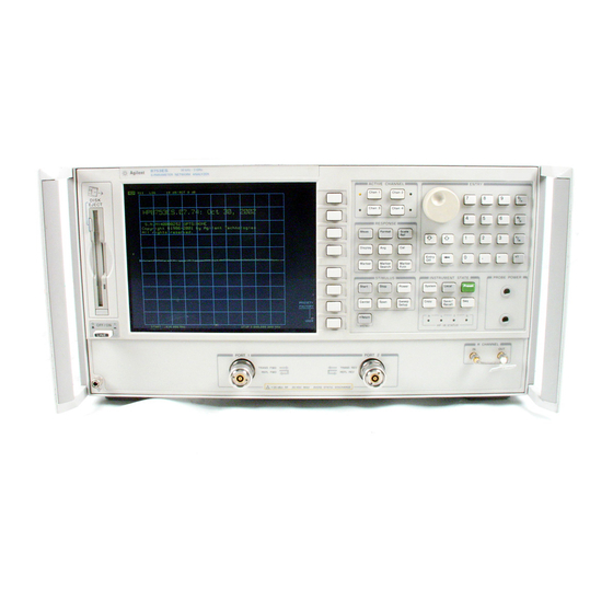
Page 29 HP 8753E Front Panel ............
Page 30 2-43. Sloping Limit Lines 2-50 2-44. Example Single Points’Lk’Line : 1 : 1 1 1 1 1 1 : : : : : 1 1 1 1 1 : 1 : 2-51 2-45. Example Stimulus Offset of Limit Lines ....2-54 .
Page 31 4-2. Printing Two Measurements ......4-3. Peripheral Connections to the Analyzer ....4-4.
Page 32 6-77 6-52. HP 87533 functional block diagram for a 2-port error-corrected measurement system ....... . .
Page 33 11-17 11-2. HP-IB Bus Structure ......11-3. AnaIyzer Siie Bus Concept ......
Page 34 6-13. Gate Characteristics ......7-2. Measurement Port Characteristics (Corrected*) for HP 8753E (509) with 7-mm Test Ports .
Page 35 9-76 9-2. Softkey Locations ........... . 11-6 .
Page 36 Chapter 6, “Application and Operation Concepts, ’ contains explanatory-style information about many applications and analyzer operation. HP 5753E Description and Options...
Page 37 Analyzer Description The HP 8753E is a high performance vector network analyzer for laboratory or production measurements of reflection and transmission parameters. It integrates a high resolution synthesized RF source, an S-parameter test set, and a four-channel three-input receiver to measure and display magnitude, phase, and group delay responses of active and passive networks.
Page 38 Power meter calibration that allows you to use an HP-IB compatible power meter to monitor and correct the analyzer’s output power at each data point. (The analyzer stores a power correction table that contains the correction values.)
Page 39: Hp 8753E Description And Options
If the line switch is mistakenly pushed, the instrument will be turned off, losing all settings and data that have not been saved. Figure l-l. HP 8753E Front Panel F’igure l-l shows the location of the following front panel features and key function blocks.
Page 40 The @Ki) and @iGZ) keys retain a history of the last active channel. For example, if channel 2 has been enabled after channel 3, you can go back to channel 3 without pressing [Ghan’ twice. HP 5753E Dessription and Options...
Page 41 (Option 002) time domain transform (Option 010) HP-IB STATUS indicators are also included in this block. user preset state that can be dellned. Refer to the “Preset State and Memory Allocation” chapter for a complete listing of the instrument preset condition.
Page 42: Analyzer Display
The start frequency of the source in frequency domain measurements. The lower power value in power sweep. When the stimulus is in center/span mode, the center stimulus value is shown in this space. The color of the stimuhis display reflects the current active channel. HP 6753E Description and Options...
Page 43 Operation” in Chapter 6, “Application and Operation Concepts. “) Gating is on (time domain Option 010 only). (For time domain measurement procedures, refer to Chapter 2, “Making Measurements.” For time domain theory, refer to Chapter 6 “Application and Operation Concepts.“) 1-8 HP 6753E Description and Options...
Page 44 For multiple-graticule displays, the channel information labels will be in the same relative position for each graticule. The label of the active channel is enclosed in a rectangle to differentiate it Note from inactive channels. HP 6753E Description and Options...
Page 45 Measured Input(s). This shows the S-parameter, input, or ratio of inputs currently measured, as selected using the LMeas) key. Also indicated in this area is the current display memory status. Format. This is the display format that you selected using the (Format] key. 10.
Page 46: Rear Panel Features And Connectors
Power cord receptacle, with fuse. For information on replacing the fuse, refer to the Line voltage selector switch. For more information refer to the HP 87533 Network 10 ME PRECISION REFERENCE OUTPUT. (Option lD5) 10 MHZ REFERENCE ADJUST.
Page 47 Pass: TTLhigh Fail: ITLlow TEST SET INTEECONNECC. This allows you to connect an HP 8763E Option 011 analyzer to an HP 85046A/B or 85047A S-parameter test set using the interconnect cable supplied with the test set. The S-parameter test set is then fully controlled by the analyzer.
Page 48: Analyzer Options Available
Option lCM, Rack Mount Flange Kit Without Handles Option 1CM is a rack mount kit containing a pair of flanges and the necessary hardware to mount the instrument, with handles detached, in an equipment rack with 482.6 mm (19 inches) horizontal spacing. HP 8753E Description and Options...
Page 49: Option Lcp, Rack Mount Flange Kit With Handles
Option lCP, Rack Mount Flange Kit With Handles Option 1CP is a rack mount kit containing a pair of flanges and the necessary hardware to mount the instrument with handles attached in an equipment rack with 482.6 mm (19 inches) spacing.
Page 50: Differences Among The Hp 8753 Network Analyzers
Differences among the HP 8753 Network Analyzers Feature Fully integrated measurement system (built-in test s&J Auto/manual power m selecting Port power coupliug/uncoupling Internal disk drive Precision frequency reference (Option lD5) 300 kHz Frequency range - low end 300 kHz Ext. freq. range to 6 GHz (Option 006)
Page 51 300 lcHz to 3 GHz, without option 006, or 30 lcHz to 6 GHz, with Option 006 For this network analyze5 the feature is dependent on the test set being used.
Page 52: Where To Look For More Information
This Chapter contains the following example procedures for making measurements or using particular functions: Basic measurement sequence and example Four-Parameter Display Mode Magnitude and insertion phase response Electrical length and phase distortion Deviation from linear phase Group delay Limit testing Gain compression Measurements using the swept list mode Tuned Receiver Mode...
Page 53: Principles Of Microwave Connector Care
This type of information is typically located in Chapter 3 of the calibration kit manuals. For additional connector care instruction, contact your local Hewlett-Packard Sales and Service Office about course numbers HP 8505OA + 24A and HP 8505OA + 24D. See the following table for quick reference tips about connector care.
Page 54: Basic Measurement Sequence And Example
Basic Measurement Sequence and Example Basic Measurement Sequence There are five basic steps when you are making a measurement. 1. Connect the device under test and any required test equipment. Damage may result to the device under test if it is sensitive to the analyzer’s Caution default output power level.
Page 55: Setting The Source Power
Note You could also press the @ and &TJ keys and enter the frequency range limits as start frequency and stop frequency values Setting the Source Power. You could also press ~~~~.~~~~~~~~ ~~~~~~:~,~~~~~ and select of the Note power ranges to keep the power setting within the deGned range. Setting the Measurement.
Page 56: Step 4. Measure The Device Under Test
Caution Do not mistake the Iine switch for the disk eject button. See the figure below. If the Iine switch is mistakenly pushed, the instrument wiIi be turned off, losing ah settings and data that have not been saved. Step Measure the device under test.
Page 57: Using The Display Functions
Using the Display Functions In some cases, you may want to view more than one measured parameter at a time. Simultaneous gain and phase measurements for example, are useful in evaluating stability in negative feedback amplifiers. You can easily make such measurements using the dual channel display.
Page 58: Lb View The Measurement Data And Memory Trace
3. To return to a single-graticule display, press: ~~~~~~~;.,~~~~~~~,,, $8, . You can control the stimulus functions of the two channels independent of each Note Press (j) ~~~~~~~~~~ to store the current active measurement data in the memory of the active channel. The data trace is now also the memory trace.
Page 59 You can use this feature for ratio comparison of two traces, for example, measurements of gain or attenuation. 1. You must have already stored a data trace to the active channel memory, as described in “To Save a Data Trace to the Display Memory.” 2.
Page 60: 2-4. Example Of A Display Title
. ii i If you have a DIN keyboard attached to the analyzer, type the title you want from the keyboard. Then press (WI to enter the title into the analyzer. You can enter a title that has a maximum of 50 characters. (For more information on using a keyboard with the analyzer, refer to “Keyboards”...
Page 62: Channel Display
The display will appear as shown in F’igure 2-5. Channel 1 is in the upper left quadrant of the display, channel 2 is in the upper right quadrant, and channel 3 is in the lower half of the display. 1 7 S s p 1 9 9 8 11:13:31 1 0 dB/ R E F -50 dB .
Page 63: Channel Display
This enables channel 4 and the screen now displays four separate grids as shown in Figure 2-6. Channel 4 is in the lower-right quadrant of the screen. 2 S e p 1 9 9 8 14:is: 5 7 . 5 dB/ REF - 2 dB 1 0 dB/ R E F - 5 0 dB DUAL CHAN O N o f f...
Page 64: Quick Four-Parameter Display
13. Press (Ghan] again. Observe that the LED is flashing, indicating that channel 3 is active. 14. Rotate the front panel control knob and notice that marker 2 still moves on all four channel traces. 15. To independently control the channel markers: Press (Marker) ‘~~~~~~::::.~~, set ~jQ#$JR&~~- to UNCOUPLED.
Page 65: Required Equipment
(a 3-port device) are routed correctly. This example uses one of the following adapters to perform this function: HP 8753E Option K36 duplexer test adapter HP 8753E Option K39 3-port test adapter You must also have a set of calibration standards for performing a full 2-port calibration on your test set up.
Page 66 Note Make sure you connect the calibration standards to the Rx port of the test adapter (or a cable attached to it) for the FORWARD calibration, and the Antenna port for the REVERSE calibration. 12. When the calibration has been completed, save this state in the analyzer: 13.
Page 67: Duplexer Measurement
5 Au9 1 9 9 8 - 4 0 dB 1 0 dB/REF 1 0 dB/REF - 4 0 dB Ref 1: FWD T r a n s : F W D T r a n s : R E V Ref 1: REV ANALOG IN A u x I n p u t...
Page 68: Using Analyzer Display Markers
Using Analyzer Display Markers The analyzer markers provide numerical readout of trace data. You can control the marker search, the statistical functions, and the capability for quickly changing stimulus parameters with markers, from the (jMarker) key. Markers have a stimulus value (the x-axis value in a Cartesian format) and a response value (the y-axis value in a Cartesian format).
Page 69: Active And Inactive Markers Example
The active marker appears on the analyzer display as V. The active marker stimulus value is displayed in the active entry area. You can modify the stimulus value of the active marker, using the front panel knob or numerical keypad. All of the marker response and stimulus values are displayed in the upper right comer of the display.
Page 70: Marker Information Moved Into The Softkey Menu Area
If marker information obscures the display traces, you can turn off the softkey menu and move the marker information off of the display traces and into the softkey menu area. Pressing the backspace key @ performs this function. This is a toggle function of the backspace key. That is, pressing @ alternately hides and restores the current softkey menu.
Page 71: Ib Use Delta (A) Markers
4. Restore the softkey menu and move the marker information back onto the graticules: Press The display will be similar to Figure 2-11. 2 S e p 1 9 9 8 12:09: 4 3 5 dB.’ R E F - 2 dB -50 dB ‘...
Page 72: Marker 1 As The Reference Marker Example
and move marker 2 to any position that you want to measure in reference Figure 2-12. Marker 1 as the Reference Marker Example 4. ‘Ib change the reference marker to marker 2, press: When a reference marker is tied, it does not rely on a current trace to maintain its fixed position.
Page 73: Using The
1. To set the frequency value of a iixed marker that appears on the analyzer display, press: keypad. The marker is shown on the display as a small delta (A), smaller than the inactive marker triangles. 2. ‘RI set the response value (dl3) of a fixed marker, press: keypad.
Page 74 Using the :,~~.~:~.~~~ Key to Activate a Fixed Reference Marker Marker zero enters the position of the active marker as the A reference position. Alternatively, you can specify the fixed point with ;$$&E& .~~~;~.~~~~~~~. Marker zero is canceled by switching delta mode off. 1.
Page 75: Key
At a preset state, the markers have the same stimuhrs values on each channel, but they can be uncoupled so that each channel has independent markers. for the display channels. Choose .~~~~~~~~ if you want the analyzer to uncouple the marker stimulus .
Page 76: Example Of A Log Marker In Polar Format
2. Select the type of polar marker you want from the following choices: Choose ;&X#“?!&% if you want to view the magnitude and the phase of the active marker. The magnitude values appear in units and the phase values appear in degrees. active marker.
Page 77: Lb Set Measurement Parameters Using Markers
The marker annotation tells that the complex impedance is capacitive in the bottom half of the Smith chart display and is inductive in the top half of the display. Choose .X&@I#& if you want the analyzer to show the linear magnitude and the phase of the reflection coefficient at the marker.
Page 78: Setting The Start Frequency
Setting the Start Frequency 1. F’ress (mFctn) and turn the front panel knob, or enter a value from the front panel keypad to position the marker at the value that you want for the start frequency. the value of the active marker. 3 1 es2 588 PtHl CENTER SPAN...
Page 79: Setting The Center Frequency
1. Press @GiFFXj and turn the front panel knob, or enter a value from the front panel keypad to position the marker at the value that you want for the center frequency. marker. Figure 2-20. Example of Setting the Center Frequency Using a Marker...
Page 80: Setting The Frequency Span
Setting the Frequency Span You can set the span equal to the spacing between two markers. If you set the center frequency before you set the frequency span, you will have a better view of the area of interest. Turn the front panel knob, or enter a value from the front panel keypad to position the markers where you want the frequency span.
Page 81: Setting The Display Reference Value
Setting the Display Reference Viilue 1. Press (j.GLXGFctn_) and turn the front panel knob, or enter a value from the front panel keypad to position the marker at the value that you want for the analyzer display reference value. 2. Press ~~,~~~ to change the reference value to the value of the active marker. Figure 2-22.
Page 82: Setting The Electrical Delay
Setting the Electrical Delay This feature adds phase delay to a variation in phase versus frequency, therefore it is only applicable for ratioed inputs. 2. Press (jjFctn) and turn the front panel knob, or enter a value from the front panel keypad to position the marker at a point of interest.
Page 83: Searching For The Maximum Amplitude
These functions place the marker at an amplitude-related point on the trace. If you switch on tracking, the analyzer searches every new trace for the target point. Searching for the Maximum Amplitude trace. Figure 2-24. Searching for the Maximum Amplitude Using a Marker Example of 232 Making Measurements...
Page 84: Searching For The Minimum Amplitude
Searching for the Minimum Amplitude ii. i ..i ..T i . ; ; ; ..; ..s ..: : . / i . . . minimum point on the measurement trace.
Page 85: Searching For A 'Lhrget Amplitude
Searching for a ‘beget Amplitude trace. 3. If you want to change the target amplitude value (default is -3 dB), press ~~~~~ and enter the new value from the front panel keypad. 4. If you want to search for multiple responses at the target amplitude value, press .
Page 86: Searching For A Bandwidth
Searching for a Bandwidth The analyzer can automatically calculate and display the -3 dB bandwidth (BW:), center frequency (CENT:), Q, and loss of the device under test at the center frequency. (Q stands for “quality factor,” defined as the ratio of a circuit’s resonant frequency to its bandwidth.) These values are shown in the marker data readout.
Page 87: Ri Calculate The Statistics Of The Measurement Data
This function calculates the mean, standard deviation, and peak-to-peak values of the section of the displayed trace between the active marker and the delta reference. If there is no delta reference, the analyzer calculates the statistics for the entire trace. 2.
Page 88: Measuring Magnitude And Insertion Phase Response
Measuring Magnitude and Insertion Phase Response The analyzer allows you to make two different measurements simultaneously. You can make these measurements in different formats for the same parameter. For example, you could measure both the magnitude and phase of transmission. You could also measure two different parameters (Sll and S&.
Page 89: Measuring Insertion Phase Response
4. Reconnect your test device. 5. lb better view the measurement trace, press: . . . , . , . _ . , . . , . , . / ../ ..6.
Page 90: Phase Samples
The phase response shown in F’igure 2-32 is undersampled; that is, there is more than HO0 phase delay between frequency points If the A4 2 HO”, incorrect phase and delay information may result. Figure 2-32 shows an example of phase samples being with A+ less than MO0 and greater than MOO.
Page 91: Measuring Electrical Length And Phase Distortion
Measuring Electrical Length and Phase Distortion Electrical Length The analyzer mathematically implements a function similar to the mechanical “line stretchers” of earlier analyzers. This feature simulates a variable length lossless transmission line, which you can add to or remove from the analyzer’s receiver input to compensate for interconnecting cables, etc.
Page 92: Linearly Changing Phase
3. Substitute a thru for the device and perform a response calibration by pressing: Reconnect your test device. 5. To better view the measurement trace, press: Notice that in Figure 2-34 the SAW filter under test has considerable phase shift within only a 2 MHz span.
Page 93: Measuring Phase Distortion
8. Press (-Ref) ~~~~~~~~~~ ad turn the front panel knob to increase me ele&ricd length until you achieve the best flat line, as shown in Figure 2-35. The measurement value that the analyzer displays represents the electrical length of your device relative to the speed of light in free space.
Page 94: Group Delay
Follow the procedure in “Measuring Electrical Length.” ..To use the marker statistics to measure the maximum peak-to-peak deviation from linear phase, press: M a r k e r F c t n ~~.:~~~~~~ ,f!@@ Activate and adjust the electrical delay to obtain a minimum peak-to-peak value. Note It is possible to use delta markers to measure peak-to-peak deviation in only one portion of the trace, see “lb Calculate the Statistics of the Measurement...
Page 95: Group Delay Example Measurement
3. lb activate a marker to measure the group delay at a particular frequency, press: Figure 2-37. Group Delay Example Measurement Group delay measurements may require a specific aperture (AF’) or frequency spacing between measurement points The phase shift between two adjacent frequency points must be less than 4.
Page 96 5. lb increase the effective group delay aperture, by increasing the number of measurement points over which the analyzer calculates the group delay, press: As the aperture is increased the “smoothness” of the trace improves markedly, but at the expense of measurement detail. Figure 2-39.
Page 97: Setting Up The Measurement Parameters
Limit testing is a measurement technique that compares measurement data to constraints that you define. Depending on the results of this comparison, the analyzer will indicate if your device either passes or fails the test. Limit testing is implemented by creating individual flat, sloping, and single point limit lines on the analyzer display.
Page 98: Creating Flat Limit Lines
4. Reconnect your test device. 5. To better view the measurement trace, press: S c a l e R e f ... ;:: /,,,,, i ....1 :$?&% : Creating Flat Limit Lines In this example procedure, the following flat Iimit Iine values are set: Frequency Range ..............
Page 99 5. To terminate the flat line segment by establishing a single point limit, press: Figure 2-41 shows the flat limit lines that you have just created with the following parameters: stimulus from 127 MHz to 140 MHz upper limit of -21 dB lower limit of -27 dB Figure 2-41.
Page 100: Creatingaslopinglimitline
Figure 2-42. Example Flat Limit Lines Creating a Sloping Limit Line This example procedure shows you how to make limits that test the shape factor of a SAW Frequency Bange ..............Power Range 144 MHz to 146 MHz ............To establish the start frequency and limits for a sloping limit line that tests the low side of the filter, press: Making Measurements 249...
Page 101: Sloping Limit Lines
... . . i xi ..i ..the l?lter, press: You could use this type of limit to test the shape factor of a ITIter. Figure 2-43.
Page 102: Creating Single Point Limits
Creating Single Point Limits In this example procedure, the following limits are set: from -23 dB to -28.5 dB at 141 MHz from -23 dB to -28.5 dB at 126.5 MHz Figure 2-44. Example Single Points Limit Line Making Measurements 2-51...
Page 103: Editing Limit Segments
Editing Limit Segments This example shows you how to edit the upper limit of a limit line. 1. To access the limits menu and activate the limit lines, press: 2. symbol (>) on the analyzer display to the segment you wish to modify, press: 3.
Page 104: Reviewing The Limit Line Segments
1. To access the limits menu and activate the limit lines, press: Reviewing the Limit Line Segments The limit table data that you have previously entered is shown on the analyzer display. 2. To verify that each segment in your limits table is correct, review the entries by pressing: 3.
Page 105: Offsetting Limit Lines
Offsetting Limit Lines The limit offset functions allow you to adjust the limit lines to the frequency and output level of your device. For example, you could apply the stimulus offset feature for testing tunable This example shows you the offset feature and the limit test failure indications that can appear on the analyzer display.
Page 106: Measuring Gain Compression
Measuring Gain Compression Gain compression occurs when the input power of an amplifier is increased to a level that reduces the gain of the amplifier and causes a nonlinear increase in output power. The point at which the gain is reduced by 1 dB is called the 1 dB compression point. The gain compression will vary with frequency, so it is necessary to find the worst case point of gain compression in the frequency band.
Page 107 b. To uncouple the channel stimulus so that the channel power will be uncoupled, press: This will allow you to separately increase the power for channel 2 and channel 1, so that you can observe the gain compression on channel 2 while channel 1 remains unchanged.
Page 108 14. To set the CW frequency before going into the power sweep mode, press: 16. Enter the start and stop power levels for the sweep. Now channel 1 is displaying a gain compression curve. (Do not pay attention to channel 2 at this time.) 17.
Page 109: Gain Compression Using Power Sweep
2 dB/ REF 1 9 0 1 dB I og 1 3 2 dBm I og MRG 5 dB/ R E F 0 dB 7 . 6 4 7 4 1 dB comd 1 .OOO 000 MHz S T O P 0 .
Page 110: Measuring Gain And Reverse Isolation Simultaneously
Measuring Gain and Reverse Isolation Simultaneously Since an amplifier will have high gain in the forward direction and high isolation in the reverse direction, the gain (E&l) will be much greater than the reverse isolation (SH.). Therefore, the power you apply to the input of the amplifier for the forward measurement (SZl) should be considerably lower than the power you apply to the output for the reverse measurement saturated.
Page 111: Gain And Reverse Isolation
Note the calibration. However, the analyzer compensates for nominal power changes you make during a measurement, so that the error correction still remains approximately valid. In these cases, the Cor annunciator will change to CA. START 1 . 0 0 0 0 0 0 MHz S T O P 1 0 0 0 000 0 0 0 MHz Figure 2-49.
Page 112: Measurements Using The Swept List Mode
Measurements Using the Swept List Mode When using a list frequency sweep, the HP 8753E has the ability to sweep arbitrary frequency segments, each containing a list of frequency points. Two different list frequency sweep modes can be selected: In this mode, the source steps to each defined frequency point, Stepped List Mode stopping while data is taken.
Page 113: Observe The Characteristics Of The Filter
Observe the Characteristics of the Filter Figure 2-51. Characteristics of a Filter needed to avoid overdriving the next stage of the DUT (if that stage contains an amplifier) or the network analyzer receiver. characteristic, the dynamic range of the system will have to be maximized. This can be done by increasing the incident power and narrowing the IF bandwidth.
Page 114: Set Up The Lower Stopband Parameters
Set Up the Lower Stopband Parameters 3. lb set up the segment for the lower stopband, press 4. ‘Ib maximize the dynamic range in the stopband (increasing the incident power and narrowing the IF bandwidth), press 6. ‘RI specify a lower power level for the passband, press .
Page 115: Calibrate And Measure
8. Tbmaximiz e the dynamic range in the stopband (increasing the incident power and narrowing the IF bandwidth), press: . . . , . : . : . : ..< : ; . . , : , : : : : : : . y . . : . . . : . : . . : : . < Calibrate and Measure Remove the DUT and perform a full two-port calibration.
Page 116: Filter Measurement Using Swept List Mode
Filter Measurement Using Linear Sweep (Power: 0 dBm/lF BW: 3700 Hz) SEGMENT I SEGMENT 3 Power: +I 0 dBm Power: +lO dBm IF BW: 1000 Hz IF BW: 300 Hz Power: -10 dBm IF BW: 3700 Hz Figure 2-53. Filter Measurement Using Swept List Mode Making Measurements 245...
Page 117: Measurements Using The Tuned Receiver Mode
Measurements Using the Tuned Receiver Mode In the tuned receiver mode, the analyzer’s receiver operates independently of any signal source. This mode is not phase-locked and functions in all sweep types. The analyzer tunes the receiver to a synthesized CW input signal at a precisely specified frequency. All phase lock routines are bypassed, increasing sweep speed significantly.
Page 118: External Source Requirements
External Source Requirements An analyzer in tuned receiver mode can receive input signals into PORT 1, PORT 2, or R CHANNEL IN. Input power range specifications are provided in Chapter 7, ( L Specifications and Measurement Uncertainties. n Making Measurements 247...
Page 119: Test Sequencing
Test sequencing allows you to automate repetitive tasks. As you make a measurement, the analyzer memorizes the keystrokes. Later you can repeat the entire sequence by pressing a single key. Because the sequence is defined with normal measurement keystrokes, you do not need additional programming expertise.
Page 120: Creating A Sequence
Creating a Sequence 1. ‘lb enter the sequence creation mode, press: As shown in F’igure 2-55, a list of instructions appear on the analyzer display to help you create or edit a sequence. Figure 2-55. ‘l&t Sequencing Help Instructions 2. ‘RI select a sequence position in which to store your sequence, press: This choice selects sequence position #l.
Page 121: Running A Sequence
3. To create a test sequence, enter the parameters for the measurement that you wish to make. For this example, a SAW filter measurement is set up with the following parameters: The above keystrokes will create a displayed list as shown: Start of Sequence RECALLPRSTSTATE LOG MAG...
Page 122: Editing A Sequence
Editing a Sequence Deleting Commands 1. To enter the creation/editing mode, press: 2. ‘Ib select the particular test sequence you wish to modify (sequence 1 in this example), press: . . , . ; .., . . , . , / _ . , . . , . 3.
Page 123: Modifying A Command
Modifying a Command 1. To enter the creation/editing mode, press: 2. To select the particular test sequence you wish to modify, (sequence 1 in this example), press: ..i i i ..A . . v . : . w The following list is the commands entered in “Creating a Sequence.’...
Page 124: Changing The Sequence Title
Changing the Sequence Title If you are storing sequences on a disk, you should replace the default titles (SEQl, SEQ2 . . . ). To select a sequence that you want to retitle, press: ..~ . ~ ~ ~ . ~ . ~ ~ ~ . “ . ~ ~ ~ ~ ~ . ~ ~ ..: : ~ ~ ~ . . . The analyzer shows the available title characters.
Page 125: Storing A Sequence On A Disk
Storing a Sequence on a Disk 1. To format a disk, refer to Chapter 4, “Printing, Plotting, and Saving Measurement Results.” 2. To save a sequence to the internal disk, press: ....: . ..:: i: The disk drive access light should turn on briefly.
Page 126: Loading A Sequence From Disk
Loading a Sequence from Disk For this procedure to work, the desired file must exist on the disk in the analyzer drive. 1. To view the first six sequences on the disk, press: If the desired sequence is not among the Rrst six files, press: :: .
Page 127: Cascading Multiple Example Sequences
Cascading Multiple Example Sequences By cascading test sequences, you can create subprograms for a larger test sequence. You can also cascade sequences to extend the length of test sequences to greater than 200 lines In this example, you are shown two sequences that have been cascaded. You can do this by having the last command in sequence 1 call sequence position 2, regardless of the sequence title.
Page 128: Loop Counter Example Sequence
Loop Counter Example Sequence This example shows you the basic steps necessary for constructing a looping structure within a test sequence. A typical application of this loop counter structure is for repeating a specific measurement as you step through a series of CW frequencies or dc bias levels For an example application, see “Fixed IF Mixer Measurements”...
Page 129: Generating Files In A Loop Counter Example Sequence
Generating Files in a Loop Counter Example Sequence This example shows how to increment the names of tiles that are generated by a sequence with a loop structure. Start of Sequence LOOP COUNTER 7 xl INTERNAL DISK DATA ONLY DO SEQUENCE SEQUENCE 2...
Page 130: Limit Test Example Sequence
Start of Sequence FILE NAME PLOT NAME SINGLE SAVE FILE 0 PLOT DECR LOOP COUNTER IF LOOP COUNTER 0 THEN DO SEQUENCE 2 Sequence 1 initializes the loop counter and calls sequence 2. Sequence 2 repeats until the loop counter reaches 0. It takes a single sweep, saves the data file and plots the display. The data file names generated by this sequence will be: through The plot llle names generated by this sequence will be:...
Page 131 This will create a displayed list for sequence 1, as shown: Start of Sequence RECALL FlEG 1 IF LIMIT TEST PASS THEN DO IF LIMIT TEST FAIL THEN DO 2. lb create a sequence that stores the measurement data for a device that has passed the limit test, press: This will create a displayed list for sequence 2, as shown: Start of Sequence...
Page 132: Measuring Swept Harmonics (Option 002 Only)
Measuring Swept Harmonics (Option 002 Only) The analyzer has the unique capability of measuring swept second and third harmonics as a function of frequency in a real-time manner. Figure 2-56 displays the absolute power of the fundamental and second harmonic in dBm. Figure 2-57 shows the second harmonic’s power level relative to the fundamental power in dBc Follow the steps listed below to perform these measurements.
Page 133: Nd Harmonic Power Level In Dbc
I og MRG S dB/ R E F 0 dB 7 . 6 7 4 2 CHZ START 1 6 . 0 0 0 0 0 0 MHz STOP 1 0 0 0 . 0 0 0 0 0 0 MHz Figure 2-57.
Page 134: Measuring A Device In The Time Domain (Option 010 Only)
Measuring a Device in the Time Domain (Option 010 Only) The HP 8753E Option 010 allows you to measure the time domain response of a device. Time domain analysis is useful for isolating a device problem in time or in distance. Time and distance are related by the velocity factor of your device under test.
Page 135: Time Domain Transmission Example Measurement
2. ‘lb choose the measurement parameters, press: 3. Substitute a thru for the device under test and perform a frequency response correction. Refer to “Calibrating the Analyzer,” located at the beginning of this Chapter, for a detailed procedure. 4. Reconnect your device under test. 5.
Page 136 8. To access the gate function menu, press: To set the gate parameters, by entering the marker value, press: center gate marker. “T” As shown in Figure 2-60, only response from the main path is displayed. You may remove the displayed response from inside the gate markers by Note pressing ;Sga:’...
Page 137 Gate spfm Gate Span Minimum -68 dB Normal -57 dB Wide fO.l dB -70 dB I NOTE: With 1601 frequency points, gating is available only in the bandpass mode. The passband ripple and sidelobe levels are descriptive of the gate shape. The cutoff time is the time between the stop time (-6 dB on the filter skirt) and the peak of the first sidelobe, and is equal on the left and right side skirts of the hlter.
Page 138: Gating Effects In A Frequency Domain Example Measurement
Figure 2-62. Gating Effects in a Frequency Domain Example Measurement Making Measurements 2-87...
Page 139: Reflection Response In Time Domain
Reflection Response in Time Domain The time domain response of a reflection measurement is often compared with the time domain reflectometry (TDR) measurements. Like the TDR, the analyzer measures the size of the reflections versus time (or distance). Unlike the TDR, the time domain capability of the analyzer allows you to choose the frequency range over which you would like to make the measurement.
Page 140: Device Response In The Frequency Domain
4. To better view the measurement trace, press: ..complex ripple pattern is caused by reflections from the adapters interacting with each other. By transforming this data to the time domain, you can determine the magnitude of the reflections versus distance along the cable.
Page 141: Device Response In The Time Domain
7. To enter the relative velocity of the cable under test, press: and enter a velocity factor for your cable under test. Most cables have a relative velocity of 0.66 (for polyethylene dielectrics) or 0.7 Note (for teflon dielectrics). If you would like the markers to read actual one-way distance rather than return trip distance, enter one-half the actual velocity factor.
Page 142: Non-Coaxial Measurements
Non-coaxial Measurements The capability of making non-coaxial measurements is available with the HP 8753 family of analyzers with TRL* (thru-reflect-line) or LRM* (line-reflect-match) calibration. For in-depth information on TRL*/LRM* calibration, refer to Chapter 6, “Application and Operation Concepts. n Non-coaxial, on-wafer measurements present a unique set of challenges for error correction in the analyzer: of isolation between the input and the output.
Page 143: Making Mixer Measurements
This chapter contains information and example procedures on the following topics: Measurement considerations ..Reducing the effect of spurious responses Eliminating unwanted mixing and leakage signals How RF and IF are dellned Frequency offset mode operation Differences between internal and external R channel inputs Power meter calibration Conversion loss using the frequency offset mode High dynamic range swept RF/IF conversion loss...
Page 144: Measurement Considerations
Measurement Considerations into consideration: ..Reducing the Effect of Spurious Responses Eliminating Unwanted Mixing and Leakage Signals Analyzer Operation How RF and IF Are Defined Frequency Offset Mode Operation Differences Between Internal and External R channel Inputs Rower Meter Calibration Minimizing Source and Load Mismatches When characterizing linear devices, you can use vector accuracy enhancement to...
Page 145: Up Converter Port Connections
In a down converter measurement where the ~~~,~~~~~~ softkey is selected, the notation on the analyzer’s setup diagram indicates that the analyzer’s source frequency is labeled RF, connecting to the mixer RF port, and the analyzer’s receiver frequency is labeled IF, connecting to the mixer IF port.
Page 146: Frequency Offset Mode Operation
Frequency Offset Mode Operation Frequency offset measurements do not begin until all of the frequency offset mode parameters are set. These include the following: Start and Stop IF Frequencies Up Converter / Down Converter The LO frequency for frequency offset mode must be set to the same value as the external LO source.
Page 147 Figure 3-3. B Channel External Connection 4. Measure the output power in the R channel by pressing: Observe the 13 to 16 dR offset in measured power. The actual input power level to the R channel input must be 0 dBm or less, -10 dRm typical, to avoid receiver saturation effects The minimum signal level must be greater than -35 dBm to provide sufficient signal for operation of the phaselock loop.
Page 148: Power Meter Calibration
Power Meter Calibration Mixer transmission measurements are generally configured as follows: measured output power (watts) /set input power (Watts) measured output power (d&n) - set input power (dBm) For this reason, the set input power must be accurately controlled in order to ensure measurement accuracy.
Page 149: Conversion Loss Using The Frequency Offset Mode
Conversion Loss Using the Frequency Offset Mode Conversion loss is the measure of efficiency of a mixer. It is the ratio of side-band IF power to RF signal power, and is usually expressed in dB. (‘lb express ratios in dR, denominator must be subtracted from the dBm power in the numerator.) The mixer translates the incoming signal, (RF), to a replica, (IF), displaced in frequency by the local oscillator, (Lo>.
Page 151: Connections For A One-Sweep Power Meter Calibration For Mixer Measurements
11. lb perform a one sweep power meter calibration over the IF frequency range at 0 dBm, press: Note Because power meter calibration requires a longer sweep time,...yyou may want to reduce the number of points before pressing ~~~;~~~~. After the power meter calibration is finished, return the number of points to its originaI Once completed, the display should read 0 dBm.
Page 152: Diagram Of Measurement Frequencies
15. To select the converter type and a high-side Lo measurement configuration, press: Notice in this high-side LO, down conversion configuration, the analyzer’s source is actuahy sweeping backwards, as shown in Figure 3-7. The measurement setup diagram is shown in Figure 3-8.
Page 153: Conversion Loss Example Measurement
18. ‘lb view the conversion loss in the best vertical resolution, press: Figure 3-9. Conversion Loss Example Measurement In this measurement, you set the input power and measured the output power. Figure 3-9 shows the absolute loss through the mixer versus mixer output frequency. If the mixer under test contained built-in amplification, then the measurement results would have shown conversion gain.
Page 154: High Dynamic Range Swept Rf/If Conversion Loss
High Dynamic Range Swept RF/IF Conversion Loss The HP 8753E’s frequency offset mode enables the testing of high dynamic range frequency converters (mixers), by tuning the analyzer’s high dynamic range receiver above or below its source, by a fixed offset. This capability allows the complete measurement of both pass and reject band mixer characteristics.
Page 155: Connections For Broad Band Power Meter Calibration
A N A L Y Z E R P O W E R M E T E R Figure 3-10. Connections for Broad Band Power Meter Calibration 4. Select the HP 8753E as the system controller: 5. Set the power meter’s address: 8. Perform a...
Page 156 9. Connect the measurement equipment as shown in Figure 3-11. Figure 3-11. Connections for Eeceiver Calibration Set the following analyzer parameters: Once completed, the analyzer should display 0 deem. Make the connections shown in Figure 3-12. Set the Lo source to the desired CW frequency and power level. For this example the values are as follows: CW frequency = 1500 MHz source power = 13 dBm...
Page 157: Connections For A High Dynamic Range Swept If Conversion Loss Measurement
N E T W O R K A N A L Y Z E R Figure 3-12. Connections for a High Dynamic Range Swept IF Conversion Loss Measurement 14. To set the frequency offset mode LO frequency, press: 15. To select the converter type and low-side Lo measurement configuration, press: In this low-side Lo, down converter measurement, the analyzer’s source frequency range determined from the following equation: receiver frequency range (100 - 1000 MHz) + Lo frequency (1500 MHz) = 1.6-2.5 GHz...
Page 158: 3-13. Example Of Swept If Conversion Loss Measurement
START 100 000 000 MHZ STOP 1 000 000 ocin MHZ Figure 3-13. Example of Swept IF Conversion Loss Measurement Making Mixer Measurements...
Page 159: Fixed If Mixer Measurements
1. Make the following connections as shown in Figure 3-14. Set the HP-IB address of the external RF source to 19 and the external Ix) source to 21. Confirm that the external sources are configured to receive commands in the SCPI programming language and that their output power is switched on.
Page 160: Connections For A Response Calibration
REFERENCE REFERENCE 10 dB 6 dB EXTERNAL EXTERNAL RF SOURCE LO SOURCE Figure 3-14. Connections for a Response Calibration 4. Press the following keys on the analyzer to create sequence 1: Note keyboard may be used for convenience. Performing a Response Calibration .
Page 161 Mixer the User to to the l&t Set Initializing a Loop Counter Value to 26 Addressing and Conflguring the Two Sources ....i i i .
Page 162 Start of Sequence RECALL PRST STATE SYSTEM CONTROLLER TUNED RECEIVER NUMBER OF POINTS DONE DONE LIST FREQ TITLE PERIPHERAL HPIB ADDR TITLE TITLE TO PERIPHERAL CALIBRATE: RESPONSE CAL STANDARD TITLE CONNECT MIXER PAUSE LOOP COUNTER SCALE/DIV REFERENCE POSITION REFERENCE VALUE MANUAL TRG ON POINT TITLE TITLE...
Page 163: Sequence 2 Setup
TITLE FREQ:MODECW;CW 6OOMHZ;:FREQ:CW:STEP 100MHZ DO SEQUENCE Sequence 2 Setup The following sequence makes a series of measurements until all 26 CW measurements are made and the loop counter value is equal to zero. This sequence includes: taking data incrementing the source frequencies labeling the screen 1.
Page 164: Connections For A Conversion Loss Using The Tuned Receiver Mode
../ . . % ..following sequence commands: Start of Sequence MANUALTRG ONPOINT TITLE PERIPHERAL HPIB ADDR PERIPHERAL HPIB ADDR DECR LOOP COUNTER TITLE MEASUREMENT COMPLETED 2.
Page 165: Example Fixed If Mixer Measurement
S T A R T 1 0 0 . 0 0 0 000 MHZ S T A R T 1 0 0 . 0 0 0 000 MHZ S T O P 1 0 0 . 0 0 0 000 M H Z S T O P 1 0 0 .
Page 166: Phase Or Group Delay Measurements
= 13 dRm Initialize the analyzer by pressing Q%+. From the front panel of the HP 8753E, set the desired receiver frequency and source output power by pressing: Connect the instruments as shown in Figure 3-17, placing a broadband “calibration” mixer...
Page 167 550 MHz LOW PASS FILTER 10 d8 10 dB REFERENCE CALIBRATION MIXER MIXER CONVERTER EXTERNAL LO SOURCE Figure 3-17. Counections for a Group Delay Measurement 5. To set the frequency offset mode LO frequency from the analyzer, press: 6. To select the converter type and a high-side LO measurement configuration, press: 7.
Page 168: Group Delay Measurement Example
8. To make a response error-correction, press: 9. Replace the “calibration” mixer with the device under test. If measuring group delay, set the delay equal to the “calibration” mixer delay (for example -0.6 ns) by pressing: 10. Scale the data for best vertical resolution. SPAN .lOO 000 000 GHz -CENTER .300 000 000 GHz Figure 3-18.
Page 169: Amplitude And Phase Tracking
Amplitude and Phase Tracking Using the same measurement setup as in “Phase or Group Delay Measurements,” you can determine how well two mixers track each other in terms of amplitude and phase. 1. Repeat steps 1 through 8 of the previous “Group Delay Measurements” section with the following exception: In step 7, select w $&I2 .
Page 170: Conversion Compression Using The Frequency Offset Mode
Conversion Compression Using the Frequency Offset Mode Conversion compression is a measure of the maximum RF input signal level, where the mixer provides linear operation. The conversion loss is the ratio of the IF output level to the RF input level.
Page 171: Connections For The First Portion Of Conversion Compression Measurement
Caution connector saver for R CHANNEL IN. NETWORK ANALYZER Figure 3-20. Connections for the First Portion of Conversion Compression Measurement 5. lb view the absolute input power to the analyzer’s R channel, press: 6. To store a trace of the receiver power versus the source power into memory and view data/memory, press: This removes the loss between the output of the mixer and the input to the receiver, and provides a linear power sweep for use in subsequent measurements...
Page 172: Connections For The Second Portion Of Conversion Compression Measurement
Caution To prevent connector damage, use an adapter (HP part number 1250-1462) as a connector saver for R CHANNEL IN. NETWORK ANALYZER MIXER UNDER TEST 3 dB EXTERNAL LO SOURCE Figure 3-21. Connections for the Second Portion of Conversion Compression Measurement 8.
Page 173: Measurement Setup Diagram Shown On Analyzer Display
The measurements setup diagram is shown in Figure 3-22. FREO OFFS NETWORK ANALYZER ON off MENU DOWN CONVERTER CONVERTER RF > LO RF < LO VIEW MEASURE RETURN CW. 200 MHz CW: BOO MHz 600 MHz 13 dBm Figure 3-22. Measurement Setup Diagram Shown on Analyzer Display 11.
Page 174: Example Swept Power Conversion Compression Measurement
Figure 3-23. Example Swept Power Conversion Compression Measurement Making Mixer Measurements...
Page 175: Isolation Example Measurements
Isolation Example Measurements Isolation is the measure of signal leakage in a mixer. Feedthrough is specificalIy the forward signal leakage to the IF port. High isolation means that the amount of leakage or feedthrough between the mixer’s ports is very small. Isolation measurements do not use the frequency offset mode.
Page 176: Connections For A Mixer Isolation Measurement
A full 2 port calibration will increase the accuracy of isolation measurements. Note Refer to Chapter 5, “Optinking Measurement Results.” 6. Make the connections as shown in Figure 3-26. NETWORK ANALYZER LOAD Figure 3-26. Connections for a Mixer Isolation Measurement 7.
Page 177: Rf Feedthrough
Figure 3-27. Example Mixer ID to RF Isolation Measurement RF Feedthrough The procedure and equipment configuration necessary for this measurement are very similar to those above, with the addition of an external source to drive the mixer’s LC port as we measure the mixer’s RF feedthrough.
Page 178: Connections For A Response Calibration
N E T W O R K A N A L Y Z E R Figure 3-28. Connections for a Response Calibration Make the connections as shown in Figure NETWORK ANALYZER SOURCE Figure 3-29. Connections for a Mixer RF Feedthrough Measurement 8.
Page 179: Example Mixer Rf Feedthrough Measurement
Figure 3-30. Example Mixer RF Feedthrough Measurement You can measure the IF to RF isolation in a similar manner, but with the following modifications: Use the analyzer source as the IF signal drive. View the leakage signal at the RF port. Making Mixer Measurements 3-37...
Page 180: Printing, Plotting, And Saving Measurement Results
Printing, Plotting, and Saving Measurement Results This chapter contains instructions for the following tasks: •I Defining a print function Plotting a measurement to disk Outputting plot hles from a PC to a plotter Outputting plot files from a PC to an HPGL compatible printer Plotting Multiple Measurements per page from disk Titling the displayed measurement Aborting a print or plot process...
Page 181: Where To Look For More Information
Chapter 2, “Making Measurements, n contains step-by-step procedures for making measurements or using particular functions. corresponding HP-IB commands. Chapter 11, “Compatible Peripherals,” lists measurement and system accessories, and other applicable equipment compatible with the analyzers An HP-IB programming overview is also included.
Page 182: Printing Or Plotting Your Measurement Results
Printing or Plotting Your Measurement Results You can print your measurement results to the following peripherals: printers with parallel interfaces You can plot your measurement results to the following peripherals: HPGL compatible printers with parallel interfaces Refer to the “Compatible Peripherals” chapter for a list of recommended peripherals. All copy coniiguration settings are stored in non-volatile memory.
Page 183 ..<..: ..: : : •I #$!‘#j#@ (for use with the HP DeskJet 540 and DeskJet 85OC) Note If your DeskJet printer does not support the 100 dpi rastg~,,,tg~at and your 3. Select one of the following printer interfaces: a.
Page 184: Deiining A Print Function
. Choose :&$& if your printer has a serial (RS-232) interface, and then configure the print ..: . . . ; ..~ : : . . : ~ .., ~ . , . , . : . : . : . function as follows: b.
Page 185: Printing One Measurement Per Page
If Yim Are Using a Color Printer 2. If you want to modify the print colors, select the print element and then choose an available color. Note You can set all the print elements to black to create a hardcopy in black and white.
Page 186: Printing Multiple Measurements Per Page
Printing Multiple Measurements Per Page 1. Configure and define the print function, as explained in “Conliguring a Print Function” and “Defining a Print Function” located earlier in this chapter.., _ i..: ..I.::.:. .:::<c ,.,., 4.
Page 188 Enter the HP-IB address of the printer (default is 01), followed by @). the HP-IB bus. c. Press LLocal) and :#N!@&&$ ,,CQ#&&$ if there is an external controller connected to the HP-IB bus. the print function as follows: . . . : ..*.i;l i ..A . . s ..
Page 189: If You Are Plotting To A Pen Plotter
Choose ~~~~~~~~~~~~~~. if your plotter has an HP-IB interface, and then conllgure the plot function as follows: a. Enter the HP-IB address of the plotter (default is 05), followed by (ZJ the plot function as follows: until the correct function appears.
Page 190: If You Are Plotting To A Disk Drive
If You Are Plotting to a Disk Drive Caution Do not mistake the line switch for the disk eject button. See the llgure below. If the line switch is mistakenly pushed, the instrument will be turned off, losing all settings and data that have not been saved. D I S K E J E C T B U T T O N L L I N E S W I T C H ’...
Page 191: Defining A Plot Function
Defining a Plot Function Note The plot definition is set to default values whenever the power is cycled. However, you can save the plot definition by saving the instrument state. Choosing Display Elements 2. Choose which of the following measurement display elements that you want to appear on your plot: q Choose ~~~~,~~~~~~~~ if you wmt the measurement data trace to appear on your p1ot.
Page 192: Selecting Pen Numbers And Colors
Note Selecting Pen Numbers and Colors example, press :,~~~~~~~~~~ and then modify the pen number. The pen number selects the color if you are plotting to an HPGLIB compatible color printer. Press Ixl) after each modification. Note The following color assignments are valid for HPGL/Z compatible color printers only.
Page 193: Selecting Line Types
Selecting Line Types q Select .!!+@!xiA.~ . . . > . . h . . . ~ ...., . . : . : .., . ; : vi ; , , , , , . . ; . . . : . . : : . . + : < . : s . > : . I::.. new line type (see F’igure 4-5), followed by @.
Page 194: Choosing Scale
Choosing Scale 6. press ~&&&&& mtd the selection appears that you want... . i..i ..; . . ; . ; ..A . . w; ...i. i includes space for all display annotations such as marker values and stimulus values.
Page 195: Plotting One Measurement Per Page Using A Pen Plotter
Marker Plotting One Measurement Per Page Using a Pen Plotter 1. Configure and define the plot, as explained in “Configuring a Plot Function” and “Defining a Plot Function” located earlier in this chapter. OUTPUT COMPLETED appears. 4-16 Printing, Plotting, and Saving Measurement Results...
Page 196: Plotting Multiple Measurements Per Page Using A Pen Plotter
Plotting Multiple Measurements Per Page Using a Pen Plotter 1. Configure and dehne the plot, as explained in “Configuring a Plot Function” and “DeGning a Plot Function” located earlier in this chapter. 3. Choose the quadrant where you want your displayed measurement to appear on the hardcopy.
Page 197 Printing, Plotting, and Saving Measurement Results...
Page 198: Plotting A Measurement To Disk
Plotting a Measurement to Disk The plot llles that you generate from the analyzer, contain the HPGL representation of the measurement display. The files will not contain any setup or formfeed commands. 1. Configure the analyzer to plot to disk. Press The analyzer assigns the first available default lilename for the displayed directory.
Page 199 However, this program is for use with LIF formatted disks and is written in HP BASIC. To View Plot Files on a PC Plot files can be viewed and manipulated on a PC using a word processor or graphics presentation program.
Page 200: Usingamipr0
Using AmiPro 1. Prom the FILE pull-down menu, select IMPORT PICTURE. 2. In the dialog box, change the file Type selection to HPGL. This automatically changes the Note The network analyzer does not use the sutllx *. PIT, so you may want to change the flename filter to * .
Page 201: Using Freelance
Using Freelance 1. From the FILE pull-down menu, select IMPORT. Set the file type in the dialog box to HGL. Note The network analyzer does not use the sulllx *.HGL, so you may want to change the tllename filter to *. * or some other pattern that will allow you to locate the llles you wish to import.
Page 202: Outputting Plot Files From A Pc To An Hpgl Compatible Printer
Outputting Plot Files from a PC to an HPGL Compatible Printer To output the plot files to an HPGL compatible printer, you can use the HPGL initialization sequence linked in a series as follows: hpglinit. Step 1. Store the HPGL initialization sequence a hle named exithpgl.
Page 203: Step 2. Store The Exit Hpgl Mode And Form Feed Sequence
Step 2. Store the exit HPGL mode and form feed sequence. 1. Create a test file by typing in each character as shown in the left hand column of l%ble 4-7. Do not insert spaces or linefeeds. 2. Name the file exithpgl. Command Remark Step 3.
Page 204: Outputting Multiple Plots To A Siie Page Using A Printer
Outputting Multiple Plots to a Single Page Using a Printer Refer to the “Plotting Multiple Measurements Per Page Using a Disk Drive, n located earlier in this chapter, for the naming conventions for plot files that you want printed on the same page. You can use the following batch file to automate the plot hle printing.
Page 205: Plotting Multiple Measurements Per Page From Disk
The following procedures show you how to store plot files on a LIF formatted disk. A naming convention is used so you can later run an HP BASIC program on an external controller that will output the flies to the following peripherals:...
Page 206 6. Define the next measurement plot that you will be saving to disk. saved. 8. Press cm) and turn the front panel knob to highlight the name of the hle that you just saved.., i,,;; , , , . , . , . , . , . , . , . , . , , . , , , . . , . , . , , . , _ _ : . x . x ; ; . : .,,i//,,,_,,i,, ; ; : , , , , ; ; , . , ; , : : : : : . ; : . : . ; : . : . : . : . : . ~ ~ , , , , . , . :::>,.- to the B character.
Page 207: Plot Quadrants
1. Deilne the plot, as explained in “Defining the Plot Function” located earlier in this chapter. 3. Choose the quadrant where you want your displayed measurement to appear on the hardcopy. The selected quadrant appears in the brackets under S$Ig#IJlJ&. .
Page 208: Titling The Displayed Measurement
Titling the Displayed Measurement You can create a title that is printed or plotted with your measurement result. 1. press I-) ~$&#@~ /&&$ to access the title menu..: ; : : . . . A : ..i ..: . ~ ..; ; ; ; ; . . . 3.
Page 209: Abortingaprintorplotprocess
You can set a clock, and then activate it, if you want the time and date to appear on your hardcopies......,.. ;..: Aborting a Print or Plot Process 1.
Page 210 3. Repeat the previous two steps until you have created hardcopies for all the desired pages of listed values. If you are printing the list of measurement data points, each page contains 30 lines of data. The number of pages is determined by the number of measurement points that you have selected under the LMenu) key.
Page 211: Solving Problems With Printing Or Plotting
Make sure that the analyzer address setting for the peripheral corresponds to the actual HP-IB address of the peripheral. The procedure is explained earlier in this chapter. Make sure that the analyzer is in system controller mode, by pressing m the analyzer must be in the pass control mode.
Page 212: Saving And Recalling Instrument States
Saving and Recalling Instrument States Places Where Ybu Can Save analyzer internal memory floppy disk using the analyzer’s internal disk drive floppy disk using an external disk drive What You Can Save to the Analyzer’s Internal Memory The number of registers that the analyzer allows you to save depends on the size of associated error-correction sets, and memory traces.
Page 213: What You Can Save To A Computer
Instrument states can be saved to and recalled from an external computer (system controller) using HP-IB mnemonics. For more information about the specific analyzer settings that can be saved, refer to the output commands located in the “Command Reference” chapter of the HP 8753E Network Analyzer Programmer’s...
Page 214: Saving An Instrument State
@. where you want to store the instrument state llle. d. Enter the HP-IB address of the peripheral, if the default address is incorrect (default = 00). Follow the entry by pressing @. e. Press 1Local) and select one of the following: .
Page 215: Saving Measurement Results
The analyzer stores data in arrays along the processing flow of numerical data, from IF detection to display. These arrays are points in the flow path where data is accessible, usually via HP-IB. You can choose from three different arrays which vary in modification flexibility when they are recalled.
Page 216: Data Processing Flow Diagram
Measurement,” located earlier in this chapter. Choose one of the following disk drives: a. Connect an external disk drive to the analyzer’s HP-IB connector, and coniigure as follows: ... . / ... . . i. i ..~ ..~ ... . ~ ; ; .._ ‘ ; , .., ..; ; z ... A ..A . . . i i / ..A . . . w .
Page 217 Press m and select one of the following: peripheral access operations. q Choose :~~~~~~~~ to allow yowself to control the analyzer Over HP-IB and also ..a allows the analyzer to take or pass control. 4 . press (--) :~~:~~-~~~~~~~~~~ .
Page 218: Ascii Data Formats
ASCII Data Formats CITIFile (Common Instrumentation Transfer and Interchange flle) is an ASCII data format that is useful when exchanging data between different computers and instruments. CITIhles are always saved when the ASCII format has been selected as shown below: .
Page 219 The template for component data fiIes is as follows: ! comment line <data line> . . . where indicates that ah following on this Iine is a comment indicates that entries following on this Iine are parameters that are being specified frequency units...
Page 220: Re-Saving An Instrument State
Re-Saving an Instrument State If you re-save a Gle, the analyzer overwrites the existing file contents. Note You cannot re-save a file that contains data only. You must create a new file. Press the QD &) keys or the front panel knob to highl&ht the name of the file that you want to delete.
Page 221: Renamingafile
Renaming a File 2. Choose from the following storage devices: q .~~~~~~~~~ the file that you want to rename. 5. Turn the front panel knob to point to each character of the new filenam~,,,,,p~~ssing an incorrect character. After you have selected all the characters in the new fllename, press Note Renaming ties may also be done by using the optional external keyboard.
Page 222: Formatting A Disk
If the external disk is a hard disk, make sure that the disk volume number is set correctly. If the disk drive is an older HP 9122, it may not recognize the newer high density disks. Substitute the disk drive.
Page 223: Optimizing Measurement Results
Optimizing Measurement Results This chapter describes techniques and analyzer functions that help you achieve the best measurement results. The following topics are included in this chapter: Increasing measurement accuracy Interconnecting cables Reference plane and port extensions Measurement error-correction One-port reflection correction Full two-port correction Modifying calibration kit standards Power meter measurement calibration...
Page 224: Where To Look For More Information
Where to Look for More Information Additional information about many of the topics discussed in this chapter is located in the following areas: measurements or using particular functions. Chapter 4, “Printing, Plotting, and Saving Measurement Results,” contains instructions for saving to disk or to the analyzer internal memory, and printing and plotting displayed measurements.
Page 225: Frequency Drift
Refer to the HP 8753E Service Guide for the measurement verification procedure. Reference Plane and Port Extensions Use the port extension feature to compensate for the phase shift of an extended measurement reference plane, due to such additions as cables, adapters, and Bxtures, after completing an error-correction procedure (or when there is no active correction).
Page 226: Measurement Error-Correction
Measurement Error-Correction The accuracy of network analysis is greatly influenced by factors external to the network analyzer. Components of the measurement setup, such as interconnecting cables and adapters, introduce variations in magnitude and phase that can mask the actual response of the device under test.
Page 227: Error-Correction Stimulus State
Corresponding Errors Carmeted Measurement Transmission or reflection Frequency response. Thru for transmission, open Response measurement when the highest or short for reflection. accuracy is not required. Response & isolation Transmission of high insertion loss Frequency response plus Same as response plus devices or reflection of high return isolation in transmission or isolation standard.
Page 228: Calibration Standards
Calibration Standards The quality of the error-correction is limited by two factors: (1) the difference between the model of the calibration standards and the actual electrical characteristics of those standards, and (2) the condition of the calibration standards. lb make the highest quality measurement calibration, follow the suggestions below: Inspect the calibration standards Clean the calibration standards,...
Page 229 Note State of the instrument can be yd@.ued so that in@polated ..“..” _ . . . interpolated error correction. Optimizing Measurement Results 5-7...
Page 230: Procedures For Error-Correcting Your Measurements
Procedures for Error-Correcting Your Measurements This section has example procedures or information on the following topics: frequency response correction frequency response and isolation correction one-port reflection correction full two-port correction modifying calibration kit standards power meter measurement calibration procedure Note If you are making measurements on uncoupled measurement channels, you must make a correction for each channel.
Page 231: Frequency Response Error-Corrections
Frequency Response Error-Corrections You can remove the frequency response of the test setup for the following measurements: reflection measurements combined reflection and transmission measurements Response Error-Correction for Reflection Measurements 1. Press w). 2. Select the type of measurement you want to make. If you want to make a reflection measurement on PORT 1 (in the forward direction, Sil), leave the instrument default setting.
Page 232: Measurement
NETWORK ANALYZER TEST POPT CABLES SHORT OPEN SHORT OPEN FOR S, 1 RESPONSE Figure 5-1. Standard Connections for Response Error-Correction for Reflection Measurement To measure the standard when the displayed trace has settled, press: If the calibration kit you selected has a choice between male and female calibration standards, remember to select the sex that applies to the test port and not the standard.
Page 233: Response Error-Correction For Transmission Measurements
Response Error-Correction for Transmission Measurements 1. Press LPresetJ. 2. Select the type of measurement you want to make. If you want to make a transmission measurement in the forward direction (&), press: If you want to make a transmission measurement in the reverse direction (&a), press: 3.
Page 234: Receiver Calibration
Note use an open or short standard for a transmission response correction, Note You can save or store the measurement correction to use for later measurements. Refer to the ‘Printing, Plotting, and Saving Measurement Results” chapter for procedures. 7. This completes the response correction for transmission measurements. You can connect and measure your device under test.
Page 235 Note You can save or store the measurement correction to use for later measurements. Refer to the “Printing, Plotting, and Saving Measurement Results” chapter for procedures. 7. This completes the receiver calibration for transmission measurements. You can connect and measure your device under test. Note The accuracy of the receiver calibration will be nearly the same as the test port power accuracy;...
Page 236: Frequency Response And Isolation Error-Corrections
Frequency Response and Isolation Error-Corrections removes frequency response of the test setup removes isolation in transmission measurements You can make a response and isolation correction for the following measurements: combined reflection and transmission measurements Response and Isolation Error-Correction for Reflection Measurements Although you can perform a response and isolation correction for reflection measurements, Hewlett-Packard recommends that you perform an S1l one-port error-correction;...
Page 237: Standard Connections For A Response And Isolation Error-Correction For Transmission Measurements
NETWORK ANALYZER F O R S,, R E S P O N S E F O R S22 R E S P O N S E SHORT OPEN F O R L O A D LOAD Figure 5-4. Standard Connections for a Response and Isolation Error-Correction for Reflection Measurements 8.
Page 238: Response And Isolation Error-Correction For Transmission Measurements
Response and Isolation Error-Correction for Transmission Measurements This procedure is intended for measurements that have a measurement range of greater than 1. Press IpresetJ. 2. Select the type of measurement you want to make. If you want to make a transmission measurement in the forward direction (&I), press: If you want to make a transmission measurement in the reverse direction (E&2), press: 3.
Page 239: Standard Connections For A Response And Isolation Error-Correction For Reflection Measurements
FOR RESPONSE FOR ISOLATION POSSIBLE ADAPTERS LOAD LOAD Figure 5-5. Standard Connections for a Response and Isolation Error-Correction for Transmission Measurements Note If you will be measuring highly reflective devices, such as filters, use the test device, connected to the reference plane and terminated with a load, for the isolation standard.
Page 240: One-Port Reflection Error-Correction
One-Port Reflection Error-Correction removes source match errors of the test setup You can perform a l-port correction for either an S11 or an S22 measurement. The only difference between the two procedures is the measurement parameter that you select. Note This is the recommended error-correction process for all reflection measurements, when full two-port correction is not used.
Page 241: Standard Connections For A One Port Reflection Error-Correction
NETWORK ANALYZER OPEN SHORT LOAG OPEN SHORT LOAD FOR S,, FOP Sz2 Figure 5-6. Standard Connections for a One Port Reflection Error-Correction 8. To measure the standard, when the displayed trace has settled, press: Note If the calibration kit that you selected has a choice between male or female calibration standards, remember to select the sex that applies to the test port and not the standard.
Page 242 Note You can save or store the error-correction to use for later measurements. Refer to the “Printing, Plotting, and Saving Measurement Results” chapter for procedures. 14. This completes the one-port correction for reflection measurements. You can connect and measure your device under test. Optimizing Measurement Results...
Page 243: Full Two-Port Error-Correction
Full Two-Port Error-Correction removes directivity errors of the test setup in forward and reverse directions removes source match errors of the test setup in forward and reverse directions removes isolation errors of the test setup in forward and reverse directions (optional) removes frequency response of the test setup in forward and reverse directions Note This is the most accurate error-correction procedure.
Page 244 6. To measure the standard, when the displayed trace has settled, press: WAIT -, MEXWFlING CAL STANDARD analyzer displays during the standard measurement. The analyzer underlines the @!?Zl& softkey after it measures the standard. 7. Disconnect the open, and connect a short circuit to PORT 1. 8.
Page 246: Trl Error-Correction
The HP 8753E analyzer has the capability of making calibrations using the TRL*/LRM* method. You must have a TRL calibration kit defined and saved in the :$&$%@$.T.. as shown in ....) “Modifying Calibration Kit Standards, n located later in this section.
Page 247: Trm Error-Correction
Connect a load to PORT 2, and press: Connect the load to PORT 1, and press: You may repeat any of the steps above. There is no requirement to go in the order of steps. When the analyzer detects that you have made all the necessary measurements, the .
Page 248 trace settleq,,),,press the softkey corresponding to the load used. If a sliding load is used, press ~~~~~~~~:: to access the Sliding Load menu. Position the slide and press When all the appropriate load measurements are complete, the load data is measured and Repeat the previous TRM load measurement steps for PORT 2.
Page 250 Default Standard Type Staadard Number short (m) broadband load sliding load short (f) 5. Press the underlined softkey. For example, if you selected (iJ (xl) in the previous step, Note “type” of standard. 6. This step applies only to the open. Go to the next step if you selected any other standard. analyzer front panel to change the value.
Page 251: Definitions
The part number of this product note is 5091-3645E. Although the product note was written for the HP 8510 family of network analyzers, it also applies to the HP 8753E. For a discussion on TRL calibration, refer to “TRIJLRM Calibration” in Chapter 6, “Application and Operation Concepts.”...
Page 252 4. To the purposes of this example, change the name of the standard by pressing .X&##%+$~. and modifying the name to “LINE.” When the title area shows the new label, press: Assign the Standards to the Various TRL Classes 8. ‘lb assign the calibration standards to the various TRL calibration classes, press: .
Page 253: Modifying Trm Standards
The part number of this product note is 5091-3645E. Although the product note was written for the HP 8510 family of network analyzers, it also applies to the HP 8753E. For a discussion on TRL calibration, refer to “TRL/LRM Calibration” in Chapter 6, “Application and Operation Concepts.
Page 254 4. ‘lb define the THRUAJNE standard, press: To define the LINE/MATCH standard, press: For the purposes of this example, change the name of the standard ..,/ ../ ..... . %. , : I ... A . . . A . > > . . . A . ; ; ..~ . ; ~ : ..~ . i . : : ~: : : . . . m . = i : ; : . : : : . . . ’ and then modify the name to “MATCH”.
Page 255 Note convenience..: : i . . : . . . 14. Change the label of the “TRL REFLECT” class to “TRMSHORT.” 15. Change the label of the “TRL LINE OR MATCH” class to “TRIMLOAD.” Optimizing Measurement Results 5-33...
Page 257: Entering The Power Sensor Calibration Data
Entering the Power Sensor Calibration Data Entering the power sensor calibration data compensates for the frequency response of the power sensor, thus ensuring the accuracy of power meter calibration. 1. Make sure that your analyzer and power meter are configured. Refer to the “Compatible Peripherals”...
Page 258: Deleting Frequency Segments
Deleting Frequency Segments . . . s i . i i /..% A , . , , ..: , ... . . _ ....: : . . . : : . . . : . . ; ; . : ; . . , , .., . , , , . . , , , , that you want to delete).
Page 259: Sample-And-Sweep Mode For Power Meter Calibration
1. Calibrate and zero the power meter. 2. Connect the equipment as shown in Figure 5-8. 3. Select the HP 8753E as the system controller: 4. Set the power meter’s address: 6. Set test port power to the approximate desired corrected power.
Page 260: 5-9. Continuous Correction Mode For Power Meter Calibration
Note Because power meter calibration requires a longer sweep time, you may want points to its original power meter calibration is Gnashed, return the number of value and the analyzer will automatically interpolate this calibration. Some accuracy will be lost for the interpolated points. The analyzer will use the data table for subsequent sweeps to correct the output power level at each measurement point.
Page 261 to maintain at the input to your test device. Compensate for the power loss of the power splitter or directional coupler in the setup. 4. If you want the analyzer to make more than one power measurement at each frequency .
Page 262: Noninsertable Device
Calibrating for Noninsertable Devices A test device having the same sex connector on both the input and output cannot be connected directly into a transmission test configuration. Therefore, the device is considered to be and one of the following calibration methods must be performed: adapter removal matched adapters N E T W O R K A N A L Y Z E R...
Page 263: Adapter Removal
Adapter Removal The adapter removal technique provides a means to accurately measure noninsertable devices. The following adapters are needed: Adapter A2, which mates with port 2 of the device, must be installed on test set port 2. Adapter A3 must match the connectors on the test device. The effects of this adapter will be completely removed with this calibration technique.
Page 264: Perform The 2-Port Error Corrections
Perform the Z-port Error Corrections 1. Connect adapter A3 to adapter A2 on port 2. (See Figure 5-12.) N E T W O R K ANAL’IZER REFERENCE REFERENCE PORT 1 Figure 5-12. ‘lko-Port Cal Set 1 2. Perform the 2-port error correction using calibration standards appropriate for the connector type at port 1.
Page 265: Remove The Adapter
4. Connect adapter A3 to adapter Al on port 1. (See F’igure 5-13.) N E T W O R K A N A L Y Z E R REFERENCE PORT 2 Figure 5-13. Two-Port Cd Set 2 5. Perform the 2-port error correction using calibration standards appropriate for the connector type at port 2.
Page 266 Note In the following two steps, calibration data is recalled, not instrument states. 10. kom the disk directory, choose the file associated with the port 1 error correction, then ..i 11. When this is complete, choose the hle for the port 2 error correction and press 13.
Page 267: Example Program
..i : Example Program HP-IB: 10 ! File : adaptrm. bas 20 ! This demonstrates how to do adapter removal over HP--1B. 30 ! 40 ! 50 ASSIGN 60 ! 70 ! Select internal disk. 80 !
Page 268: Matched Adapters
With this method, you use two precision matched adapters which are “equal. n lb be equal, the adapters must have the same match, ZO, insertion loss, and electrical delay. The adapters in most HP calibration kits have matched electrical length, even if the physical lengths appear different.
Page 269 Modify the Cal Kit Thru Deilnition With this method it is only necessary to use adapter B. The calibration kit thru definition is modified to compensate for the adapter and then saved as a user kit. However, the electrical delay of the adapter must hrst be found. 1.
Page 270: Making Accurate Measurements Of Electrically Long Devices
The faster the analyzer’s sweep rate, the larger AF’ becomes, and the larger the error in the test channel. The HP 8753E network analyzers do not sweep at a constant rate. The frequency range is covered in several bands, and the sweep rate may be different in each band. So if an operator sets up a broadband sweep with the minimum sweep time, the error in measuring a long device will be different in each band, and the data will be discontinuous at each band edge.
Page 271: Decreasing The Time Delay
Decreasing the Time Delay The other way to reduce AF’ is by decreasing the time delay, AT. Since AT is a property of the device that is being measured, it cannot literally be decreased. However, what can be decreased is the difference in delay times between the paths to the R channel and the B channel.
Page 272: Increasing Sweep Speed
Increasing Sweep Speed You can increase the analyzer sweep speed by avoiding the use of some features that require computational time for implementation and updating, such as bandwidth marker tracking. You can also increase the sweep speed by making adjustments to the measurement settings. The following suggestions for increasing sweep speed are general rules that you should experiment with: use swept list mode...
Page 273: Band Switch Points
3. Then switch to stepped list mode: If there is no difference between the measurements in either list mode, then use the swept If the memory trace indicates that there is more attenuation in swept list mode, it may be due to IF delay.
Page 274 1. press LAvg) j:;$*+;#r. 2. Set the IF bandwidth to change the sweep time. The following table shows the relative increase in sweep time as you decrease system bandwidth. 0.128 0.254 1 Preset condition, CF- includes retrace time. By reducing the averaging factor (number of sweeps) or switching off averaging, you can increase the analyzer’s measurement speed.
Page 275 The analyzer sweep time does not change proportionally with the number of points, but as indicated below. 0.106 0.181 0.330 1601 0.633 1 Preset condition, CF- lGHz, Span= lOOMHz, Correction Measurement speed can be improved by selecting the widest IF BW setting of Different sweep speeds are associated with the following three types of non-power sweeps.
Page 276 Offloading the error correction process to an external PC increases throughput on the network analyzer. This can be accomplished with remote only commands, Refer to the HP 87533 With the 2-port calibration on, faster measurements may be made by not measuring the reverse path for every forward sweep.
Page 277 4. ‘lb enter the number of sweeps, press: Optimizing Measurement Results 5-55...
Page 278: Increasing Dynamic Range
Increasing Dynamic Range Dynamic range is the difference between the analyzer’s maximum allowable input level and minimum measurable power. For a measurement to be valid, input signals must be within these boundaries. The dynamic range is affected by these factors: test port noise floor You can increase the analyzer’s source output power so that the test device output power is at the top of the measurement range of the analyzer test port.
Page 279: Reducing Receiver Crosstalk
Reducing Trace Noise You can use two analyzer functions to help reduce the effect of noise on the data trace: activate measurement averaging reduce system bandwidth The noise is reduced with each new sweep as the effective averaging factor increments. 2.
Page 280 DualChan. 1601 1601 Recall and SweeD* 1.298 1.468 Sweep only (no Recall)* I Single Ghan. Instrument State: CF- lGHz, Span=2MHz, IF BW=6 Hz. HP-IB comman ds sent for timing are 1 Error &rrection OFF. Error Ckmection ON. Optimizing Measurement Results...
Page 281 Understanding Spur Avoidance In the 400 MHz to 3 GHz range, where the source signal is created by heterodyning two higher frequency oscillators, unwanted spurious mixing products from the source may be present at the output. These spurs can become apparent in iilter measurements when filters have greater than 80 dB rejection.
Page 282 This chapter provides conceptual information on the following primary operations and applications that are achievable with the HP 8753E network analyzer. HP 8753E System operation Active channel keys Entry block keys Stimulus functions S-parameters Display formats Four parameter display Scale reference...
Page 283: Hp 8753E System Operation
The analyzer’s built-in synthesized source produces a swept RF signal or CW (continuous wave) signal in the range of 30 kHz to 3.0 GHz. The HP 8753E Option 006 is able to generate signals up to 6 GHz. The RF output power is leveled by an internal ALC (automatic leveling control) circuit.
Page 284: The Receiver Block
The Built-In ‘I&t Set The HP 8753E features a built-in test set that provides connections to the test device, as well as to the signal-separation devices. The signal separation devices are needed to separate the incident signal from the transmitted and reflected signals. The incident signal is applied to the R channel input through a jumper cable on the front panel.
Page 285: Data Processing Flow Diagram
The swept high frequency input signals are translated to llxed low frequency IF signals, using analog sampling or mixing techniques. (Refer to the HP 8753E Network Anuliyxer Semrice The IF signals are converted into digital data by an analog to digital converter (ADC). From this point on, ah further signal processing is performed mathematically by the analyzer microprocessors.
Page 286: Ratio Calculations
While only a single flow path is shown, two identical paths are available, corresponding to channel 1 and channel 2. When the channels are uncoupled, each channel is processed and controlled independently. Data point definition: A “data point” or “point” is a single piece of data representing a measurement at a single stimulus value.
Page 287: Pre-Raw Data Arrays
(~~~~~~~~:~~~~, there may be as many as eight raw arrays. These arrays are directly accessible via HP-IB. Notice that the numbers here are still complex pairs. Raw arrays contain the pre-raw data which has sampler and attenuator offset applied.
Page 288: Transform (Option 010 Only)
Transform (Option 010 Only) This transform converts frequency domain information into the time domain when it is activated. The results resemble time domain reflectometry (TDR) or impulse-response measurements The transform uses the chirp-Z inverse fast Fourier transform (FFI’) algorithm to accomplish the conversion. The windowing operation, if enabled, is performed on the frequency domain data just before the transform.
Page 289: Active Channel Keys
Active Channel Keys The analyzer has four channels for making measurements. Channels 1 and 2 are the primary channels and channels 3 and 4 are the auxihary channels. The primary channels can have different stimulus values (see “Uncoupling Stimulus Values Between Primary Channels,” below) but the auxiliary channels always have the same stimulus values as their primary channels.
Page 290: Enabling Auxiiiary Channels
Enabling Auxiliary Channels Once a full two-port calibration is active, the auxiliary channels can be enabled. ‘Ib enable channel 3 or 4, press: 1. @&X1) or lchan] 2. @z&iq-- Once enabled, an auxiliary channel can be made active by pressing [than) twice (for channel to the corresponding channel key.
Page 291: Units Terminator
Before you can modify a function, you must activate the particular function by pressing the corresponding front panel key or softkey. Then you can modify the value directly with the knob, the step keys, or the digits keys and a terminator. If no other functions are activated, the knob moves the active marker.
Page 292: Modifying Or Deleting Entries
[ Entry Off] You can use this key to clear and turn off the active entry area, as well as any displayed prompts, error messages, or warnings. Use this function to clear the display before printing or plotting. This key also helps prevent changing active values accidentally by moving the knob. The backspace key has two main functions: Deletes or modifies entries Hides the softkey menu...
Page 293: Stimuius Functions
Stimulus Functions S T I M U L U S W Figure 6-5. Stimulus Function Block The stimulus function block keys are used to define the source RF output signal to the test device by providing control of the following parameters: swept frequency ranges time domain start and stop times (Option 010 Only) power sweep start and stop values...
Page 294: Stimuius Menu
Stimulus Menu The (Menu) key provides access to the stimulus menu, which consists of softkeys that activate stimulus functions or provide access to additional menus. These softkeys are used to define and control all stimulus functions other than start, stop, center, and span. The following softkeys are located within the stimulus menu: n ~~~~;~~~~,,itUowsyou to specify the sweep time.
Page 295: The Power Menu
The Power Menu The power menu is used to define and control analyzer power. It consists of the following softkeys: ....~~~~~~~ provides access to the power range menu. .
Page 296: Power Range Transitions In The Automatic Mode
Note After measurement calibration, you can change the power within a range and still maintain nearly full accuracy. In some cases better accuracy can be achieved by changing the power within a range. It can be useful to set different power levels for calibration and measurement to minimize the effects of sampler compression or noise floor.
Page 297: Power Coupling Options
Power Coupling Options There are two methods you can use to couple and uncouple power levels with the HP 87533: channel coupling port coupling By uncoupling the primary channel powers, you effectively have two separate sources. Uncoupling the test ports allows you to have different power levels on each port.
Page 298: Manual Sweep Time Mode
Sweep Time automatic or manual mode is active. The following explains the difference between automatic and manual sweep time: instrument, it will remain hxed, regardless of changes to other measurement parameters. If you change measurement parameters such that the instrument can no longer maintain the selected sweep time, the analyzer will change to the fastest sweep time possible.
Page 299 time domain (Option 010 Only) Use ‘lhble 6-l to determine the minimum cycle time for the listed measurement parameters. The values listed represent the minimum time required for a CW time measurement with averaging off. Number of Points IF Bandwidth 3700 Hz 0.0025 0.0041...
Page 300 Trigger Menu The trigger menu is used to select the type and number of groups for the sweep trigger. The following is a description of the softkeys located within this menu: The notation “Hid” is displayed at the left of the graticule. If the 1 indicator is on at the left side of the display, trigger a new sweep with ‘2$&3&A$.
Page 301: Source Attenuator Switch Protection
Source Attenuator Switch Protection The programmable step attenuator of the source can be switched between port 1 and port 2 when the test port power is uncoupled, or between channel 1 and channel 2 when the channel power is uncoupled. To avoid premature wear of the attenuator, measurement configurations requiring continuous switching between different power ranges are not allowed.
Page 302: Channel Stimulus Coupling
Channel Stimulus Coupling (The inactive primary channel and its auxiliary channel takes on the stimulus values of the active primary channel.) In the stimulus coupled mode, the following parameters are coupled: frequency number of points source power number of groups IF bandwidth sweep time trigger type...
Page 303: Sweep Type Menu
Sweep Type Menu The following softkeys are located within the sweep type menu. Among them are the five sweep types available. , ~~~~~~~~.~ flows list frequencies to be entered or mo&fied using the e&t list menu md e&t The following sweep types will function with the interpolated error-correction feature (described later): linear frequency power sweep...
Page 304: Logarithmic Frequency Sweep (Hz)
Logarithmic Frequency Sweep (Hz) .._ . , . , . , . , . . . , . _ _ , . The Q,@$~ softkey activates a logarithmic frequency sweep mode. The source is stepped in logarithmic increments and the data is displayed on a logarithmic graticule.
Page 305: Stepped Edit Subsweep Menu
Stepped Edit Subsweep Menu Using the .X&g? or &&i, softkey within the edit list menu wiIl display the edit subsweep menu. This menu lets you select measurement frequencies arbitrarily. Using this menu it is possible to define the exact frequencies to be measured on a point-by-point basis. For example, the sweep could include 100 points in a narrow passband, 100 points across a broad stop band, and 50 points across the third harmonic response.
Page 306: Swept List Frequency Sweep (Hz)
Swept List Frequency Sweep (Hz) frequency sweep modes. The swept list mode allows the analyzer to sweep a list of arbitrary frequency points which are defined and modified in a way similar to the stepped list mode. However, this mode takes data while swe&ng through the defined frequency points, increasing throughput by up to 6 times over a stepped sweep.
Page 307: Setting Segment If Bandwidth
The power settings for all segments are restricted to a single power range. This prevents the attenuator from switching to different settings mid-sweep. Select the power range and then edit the list table to specify the segment powers. If the power range is selected after the list has been defined, the list settings may be affected.
Page 308: Power Sweep (Dbm)
Power Sweep (dBm) The ~~~~~.~~ softkey turns on a power sweep mode that is used to characterize power-sensitive circuits In this mode, power is swept at a single frequency, from a start power feature is convenient for such measurements as gain compression.or ,&GC (automatic gain control) slope.
Page 309: Response Function Block
Response Functions Figure 6-7. Response Function Block The following response function block keys are used to define and control the following functions of the act& &anml. The current values for the major response functions of the active channel are displayed in specific locations along the top of the display.
Page 310: S-Parameters Of A Two-Port Device
S-Parameters The (Meas) key provides access to the S-parameter menu which contains softkeys that can be used to select the parameters or inputs that define the type of measurement being performed. Understanding S-Parameters S-parameters (scattering parameters) are a convention used to characterize the way a device modifies signal flow.
Page 311: The S-Parameter Menu
This menu allows you to monitor voltage and frequency nodes, using the analog bus and internal counter. For more information, refer to Chapter 10, “Service Key Menus and Error Messages” in the HP 8753E Network Analgzer Service Guide. Conversion Menu This menu converts the measured reflection or transmission data to the equivalent complex impedance (Z) or admittance (Y) values.
Page 312: Input Ports Menu
Figure 6-9. Reflection Impedance and Admittance Conversions In a transmission measurement, the data can be converted to its equivalent series impedance or admittance using the model and equations shown in F’igure 6-10. Figure 6-10. Transmission Impedance and Admittance Conversions Note Avoid the use of Smith chart, SWR, and delay formats for display of Z and Y conversions, as these formats are not easily interpreted.
Page 313: The Format Menu
The Format Menu The @GGZ) key provides access to the format menu. This menu allows you to select the appropriate display format for the measured data. The following list identifies which formats are available by means of which softkeys: . :~~~.,:..~~~. .
Page 314: Log Magnitude Format
Phase Format .., , , . The $!?K softkey displays a Cartesian format of the phase portion of the data, measured in degrees This format displays the phase shift versus frequency. Figure 6-12 illustrates the phase response of the same IIlter in a phase-only format.
Page 315: Group Delay Format
Figure 6-13. Group Delay Format Smith Chart Format in reflection measurements to provide a readout of the data in terms of impedance. The intersecting dotted lines on the Smith chart represent constant resistance and constant reactance values, normalized to the characteristic impedance, ZO, of the system. Reactance values in the upper half of the Smith chart circle are positive (inductive) reactance, and those in the lower half of the circle are negative (capacitive) reactance.
Page 316: Polar Format
Figure 6-14. Standard and Inverse Smith Chart Formats corresponds to a particular value of both magnitude and phase. Quantities are read vectorally: the magnitude at any point is determined by its displacement from the center (which has zero value), and the phase by the angle counterclockwise from the positive x-axis. Magnitude is scaled in a linear fashion, with the value of the outer circle usually set to a ratio value of 1.
Page 317: Linear Magnitude Format
Linear Magnitude Format The i~~~:~.~:~~~~ softkey displays the linear magnitude format (see F’igure 6-16). This is a Cartesian format used for unitless measurements such as reflection coefficient magnitude p or transmission coefficient magnitude T, and for linear measurement units. It is used for display of conversion parameters and time domain transform data.
Page 318: Real Format
Real Format The X$&L softkey displays only the real (resistive) portion of the measured data on a Cartesian format (see Figure 6-18). This is similar to the linear magnitude format, but can show both positive and negative values. It is primarily used for analyzing responses in the time domain, and also to display an auxiliary input voltage signal for service purposes.
Page 319: Group Delay Principles
Group Delay Principles For many networks, the amount of insertion phase is not as important as the linearity of the phase shift over a range of frequencies The analyzer can measure this linearity and express it in two different ways: directly, as deviation from linear phase, or as group delay, a derived value.
Page 320: Rate Of Phase Change Versus Frequency
result in the group delay data. These errors can be significant for long delay devices. You can verify that A$ is ~180“ by increasing the number of points or narrowing the frequency span (or both) until the group delay data no longer changes. Figure 6-21.
Page 321 Group delay measurements can be made on linear frequency, log frequency, or list frequency sweep types (not in CW or power sweep). Group delay aperture varies depending on the frequency spacing and point density, therefore the aperture is not constant in log and list frequency sweep modes.
Page 322: Electrical Delay
Scale Reference Menu The @GiZGTj key provides access to the scale reference menu. Softkeys within this menu can be used to define the scale in which measured data is to be displayed, as well as simulate phase offset and electrical delay. The following softkeys are located within the scale reference menu. Electrical Delay The ~T~~~~~~~ softkey adjusts the electrical delay to balance the phase of the test (with cut-off frequency) in order to identify which type of transmission line the delay is being...
Page 323: Display Menu
Display Menu The CDisplay) key provides access to the display menu, which enables auxiliary channels 3 and 4, controls the memory math functions, and leads to other menus associated with display functions. The analyzer has four available memory traces, one per channel. Memory traces are totally channel dependent: channel 1 cannot access the channel 2 memory trace or vice versa.
Page 324: Dual Channel Displays
Dual Channel Mode set to 1X, the two traces are overlaid on a single graticule (see Figure 6-23a) With .EQH$%%A# set to ON and ~&&ET DISP set to 2X or 4X, the measurement data is displayed on two half-screen graticules, one above the other, (see Figure 6-2313). Current parameters for the two displays are annotated separately.
Page 325 Note Auxiliary channels 3 and 4 are permanently coupled by stimulus to primary channels 1 and 2 respectively. Decoupling the primary channels’ stimulus from each other does not affect the stimulus coupling between the auxiliary channels and their primary channels. 6 4 4 Application and Operation Concepts...
Page 326 However, there are two coniigurations that may not appear to function “properly”. Channel 1 requires one attenuation value and channel 2 requires a different value. Since one attenuator is used for both testports, this would cause the attenuator to continuously switch power ranges.
Page 327: Channel Position Softkey
Channel Position Softkey ..: . . . : . . : ..: : . . : : : ..:;:./ ..A . . .w;;>; ..A . . s ..; . . . L . . i i ....A/ ..w ..i >;:3 Channels 1 and 2 overlayed in the top graticule, and channels 3 and 4 are overlaid in the bottom graticule.
Page 328: Param Displays Menu
relationship between the keys and the channels. For example, beneath the four-grid display, [CHAN l] and [MEAS] Sll are shown in yellow. Notice that in the four-grid graphic, Chl is also yellow, indicating that the keys in yellow apply to channel 1. i .
Page 329: Memory Math Functions
Memory Math F’unctions Two trace math operations are implemented: and trace math is done immediately after error-correction. This means that any data processing done after error-correction, including parameter conversion, time domain transformation (Option OlO), scaling, etc, can be performed on the memory trace. You can also use trace math as a simple means of error-correction, although that is not its main purpose.
Page 330: Setting Default Colors
Setting Default Colors To set all the display elements to the factory-defined default colors, press ~~~~~~~~~~~~~~. Note cycling power to the instrument will reset the colors to the default color values. Blanking the Display ..) , .., Pressing ~~~~~~~~~~ switches off the analyzer display while leaving the instrument in its current measurement state.
Page 331 To change the color of a display elements, press the softkey for that element (such as en press fE&@$ and turn the analyzer front panel knob; use the step keys or the numeric keypad, until the desired color appears. If you change the text or background intensity to the point where the display is unreadable, you can the recover a readable display by turning off the analyzer and then turning it back on.
Page 332: Effect Of Averaging On A Trace
Averaging Menu The (XjJ key is used to access three different noise reduction techniques: sweep-to-sweep averaging, display smoothing, and variable IF bandwidth. All of these can be used simultaneously. Averaging and smoothing can be set independently for each channel, and the IF bandwidth can be set independently if the stimulus is uncoupled.
Page 333: Effect Of Smoothing On A Trace
Smoothing Smoothing (similar to video filtering) averages the formatted active channel data over a portion of the displayed trace. Smoothing computes each displayed data point based on one sweep only, using a moving average of several adjacent data points for the current sweep. The smoothing aperture is a percent of the swept stimulus span, up to a maximum of 20%.
Page 334: If Bandwidth Reduction
Figure 6-27. IF Bandwidth Reduction Another capability that can be used for effective noise reduction is the marker Hints statistics function, which computes the average value of part or all of the formatted trace. If your instrument is equipped with Option 085 (High Power System), another way of increasing dynamic range is to increase the input power to the test device using a booster amplifier.
Page 335 Markers The marker_) key displays a movable active marker on the screen and provides access to a series of menus to control up to five display markers for each channel. Markers are used to obtain numerical readings of measured values. They also provide capabilities for reducing measurement time by changing stimulus parameters, searching the trace for specific values, or statistically analyzing part or all of the trace.
Page 336: Marker Menu Delta Mode Menu
With the use of a reference marker, a delta marker mode is available that displays both the stimulus and response values of the active marker relative to the reference. Any of the five markers or a ilxed point can be designated as the delta reference marker. If the delta reference is one of the five markers, its stimulus value can be controlled by the user and its response value is the value of the trace at that stimulus value.
Page 337: Marker Function Menu
If the format is changed while a fixed marker is on, the fixed marker values become invalid. For example, if the value offset is set to 10 dl3 with a log magnitude format, and the format is then changed to phase, the value offset becomes 10 degrees. However, in polar and Smith chart formats, the specified values remain consistent between different marker types for those formats Thus an R+jX marker set on a Smith chart format will retain the equivalent values if it is changed to any of the other Smith chart markers.
Page 338: Measurement Calibration
Measurement Calibration Measurement calibration is an accuracy enhancement procedure that effectively removes the system errors that cause uncertainty in measuring a test device. It measures known standard devices, and uses the results of these measurements to characterize the system. This section discusses the following topics: causes of measurement errors calibration considerations effectiveness of accuracy enhancement...
Page 339: What Causes Measurement Errors
What Causes Measurement Errors? Network analysis measurement errors can be separated into systematic, random, and drift errors. Correctable systematic errors are the repeatable errors that the system can measure. These are errors due to mismatch and leakage in the test setup, isolation between the reference and test signal paths, and system frequency response.
Page 340: Source Match
directivity is independent of the characteristics of the test device and it usually produces the major ambiguity in measurements of low reflection devices. Source Match Source match is defined as the vector sum of signals appearing at the analyzer receiver input due to the impedance mismatch at the test device looking back into the source, as well as to adapter and cable mismatches and losses.
Page 341: Isolation (Crosstalk)
I Match Figure 6-31. Load Match The error contributed by load match is dependent on the relationship between the actual output impedance of the test device and the effective match of the return port (port 2). It is a factor in all transmission measurements and in reflection measurements of two-port devices. The interaction between load match and source match is less significant when the test device insertion loss is greater than about 6 dD.
Page 342: Characterizing Microwave Systematic Errors
Characterizing Microwave Systematic Errors One-Port Error Model In a measurement of the reflection coefficient (magnitude and phase) of a test device, the measured data differs from the actual, no matter how carefully the measurement is made. Directivity, source match, and reflection signal path frequency response (tracking) are the major sources of error (see Figure 6-32).
Page 343 Figure 6-34. Effective Directivity EDF Since the measurement system test port is never exactly the characteristic impedance (50 ohms), some of the reflected signal bounces off the test port, or other impedance transitions further down the line, and back to the unknown, adding to the original incident signal (I). This effect causes the magnitude and phase of the incident signal to vary as a function of &A and frequency.
Page 344: Reflection Tracking Em
All incident energy is absorbed. With S11~ = 0 the equation can be solved for Enr, the directivity term. In practice, of course, the “perfect load” is difficult to achieve, although very good broadband loads are available in the HP 87533 compatible calibration kits Figure 6-37. “Perfect Load” ‘Ikrmination Since the measured value for directivity is the vector sum of the actual directivity plus the actual reflection coefficient of the “perfect load,”...
Page 345 A c t u a l D i r e c t i v i t y A f t e r Figure 6-38. Measured Effective Directivity Next, a short circuit termination whose response is known to a very high degree is used to establish another condition (see F’igure 6-39).
Page 346 Figure 6-40. Open Circuit ?Lkrmina.tion This completes the calibration procedure for one port devices. Application and Operation Concepts...
Page 347: Device Measurement
Device Measurement Now the unknown is measured to obtain a value for the measured response, frequency (see Figure 6-41). Figure 6-41. Measured SI 1 This is the one-port error model equation solved for S 11A. Since the three errors and SLIM are now known for each test frequency, &IA can be computed as follows: For reflection measurements on two-port devices, the same technique can be applied, but the test device output port must be terminated in the system characteristic impedance.
Page 348 M E A S U R E M E N T ERRQRS Unknown Figure 6-42. Bhjor Sources of Error The transmission coefficient is measured by taking the ratio of the incident signal (I) and the transmitted signal (‘I) (see F’igure 6-43). Ideally, (I) consists only of power delivered by the source, and (T) consists only of power emerging at the test device output.
Page 349: Load Match Elf
PORT PORT MATCH MATCH Figure 6-44. Load Match Em The measured value, SLIM, consists of signal components that vary as a function of relationship between Esr and &A as well as E LF and f&2& so the input and output reflection coefficients of the test device must be measured and stored for use in the &IA error-correction computation.
Page 350: Source Match Esr
Isolation P O R T P O R T Figure 6-45. Isolation Em Thus there are two sets of error terms, forward and reverse, with each set consisting of six error terms, as follows: Directivity, Enr (forward) and Ena (reverse) Isolation, EXF and EXR Transmission Tracking, Err and Era Reflection Tracking, Em and ERR...
Page 351 FORWARD P O R T 1 P O R T 2 REVERSE RF IN Figure 6-46. Full Two-Port Error Model two-port device. Note that the mathematics for this comprehensive model use all forward and reverse error terms and measured values. Thus, to perform full error-correction for any one parameter, all four S-parameters must be measured.
Page 352 Figure 6-47. Full Two-Port Emor Model Equations In addition to the errors removed by accuracy enhancement, other systematic errors exist due to limitations of dynamic accuracy, test set repeatability, and test cable stability. switch These, combined with random errors, also contribute to total system measurement uncertainty. Therefore, after accuracy enhancement procedures are performed, residual measurement uncertainties remain.
Page 353: Calibration Considerations
Calibration Considerations Measurement Parameters Calibration procedures are parameter-specific, rather than channel-specific When a parameter is selected, the instrument checks the available calibration data, and uses the data found for that parameter. For example, if a transmission response calibration is performed for B/R, and an S11 l-port calibration for A/R, the analyzer retains both calibration sets and corrects whichever parameter is displayed.
Page 354: The Calibration Standards
The Calibration Standards During measurement calibration, the analyzer measures actual, well-defined standards and mathematically compares the results with ideal “models” of those standards. The differences are separated into error terms which are later removed during error-correction. Most of the differences are due to systematic errors-repeatable errors introduced by the analyzer, test set, and cables-which are correctable.
Page 355: Electrical Offset
Electrical Offset Some standards have reference planes that are electrically offset from the mating plane of the test port. These devices will show a phase shift with respect to frequency. ‘lhble 6-4 shows which reference devices exhibit an electrical offset phase shift. The amount of phase shift can be calculated with the formula: f = frequency 1 = electrical length of the offset...
Page 356: Typical Responses Of Calibration Standards After Calibration
mm or Type-N Male Type-N Female, Short (No Offset) mm Male Female Ofiet Short mm or Type-N Male Type-N Female, mm Male or Female C@et Open Application and Operation Concepts 6-76...
Page 357: How Effective Is Accuracy Enhancement
How Effective Is Accuracy Enhancement? The uncorrected performance of the analyzer is sufficient for many measurements However, the vector accuracy enhancement procedures described in Chapter 5, “Optinking Measurement Results, n will provide a much higher level of accuracy. Figure 6-49 through Figure 6-51 illustrate the improvements that can be made in measurement accuracy by using a more complete calibration routine.
Page 358 Figure 6-50. Response versus S 11 l-Port CMibration on Smith Chart calibration in Figure 6-51a and a full two-port calibration in Figure 6-51b. Figure 6-51. Response versus Full Two-Port Calibration Application and Operation Concepts...
Page 359: Correcting For Measurement Errors
Correcting for Measurement Errors The Local] key provides access to the correction menu which leads to a series of menus that implement the error-correction concepts described in this section. Accuracy enhancement (error-correction) is performed as a calibration step before you measure a test device. When The following softkeys are located within the correction menu: Ensuring a Valid Calibration Unless interpolated error-correction is on, measurement calibrations are valid only for a...
Page 360: Interpolated Error-Correction
Interpolated Error-correction You can activate the interpolated error-correction feature with the ~~~~~~:~~~ ~~&3$: softkey. This feature allows you to select a subset of the frequency range or a different number of points without recalibration. When interpolation is on, the system errors for the newly selected frequencies are calculated from the system errors of the original calibration.
Page 361: The Calibrate Menu
The Calibrate Menu There are twelve different error terms for a two-port measurement that can be corrected by accuracy enhancement in the analyzer. These are directivity, source match, load match, isolation, reflection tracking, and transmission tracking, each in both the forward and reverse direction.
Page 362: Trl*/Lrm* Two-Port Calibration
within the calibrate menu, provides the ability to make calibrations using the TRL or LRM method. For more information, refer to “TRL*/LRM* Calibration,” located later in this section. Application and Operation Concepts...
Page 363: Restarting A Calibration
Restarting a Calibration If you interrupt a calibration to go to another menu, such as averaging, you can continue the Cal Kit Menu The cal kit menu provides access to a series of menus used to specify the characteristics of calibration standards.
Page 364: Modifying Calibration Kits
Before attempting to modify calibration standard defhtitions, you should read application note application note is 5956-4352. Although the application note is written for the HP 8510 family of network analyzers, it also applies to the HP 8753E.
Page 365: Modify Calibration Kit Menu
4. Store the modified calibration kit. For a step by step procedure on how to modify calibration kits, refer to “Modifying Calibration Kit Standards” located in Chapter 5, “Cptimizing Measurement Results. n Modify Calibration Kit Menu . . . , . / _ _ menu.
Page 366 Standard dellnition is the process of mathematically modeling the electrical characteristics (delay, attenuation, and impedance) of each calibration standard. These electrical characteristics (coefficients) can be mathematically derived from the physical dimensions and material of each calibration standard, or from its actual measured response. The parameters of the standards can be listed in lhble 6-5.
Page 367 Each standard must be identified as one of five “types”: open, short, load, delay/thru, or arbitrary impedance. After a standard number is entered, selection of the standard type will present one of five menus for entering the electrical characteristics (model coefficients) corresponding to that standard type, such as &&.
Page 368: Specify Offset Menu
impedance (different from system ZO). o h m s . $%jJ,lQXG’ defmes the load as a sliding load. When such a load is measured during ..... .::.: : : . i calibration, the analyzer will prompt for several load positions, and calculate the ideal load value from it.
Page 369: Label Standard Menu
coax offset. The value of loss is entered as ohms/nanosecond (or Giga ohms/second) at 1 GHz. (Such losses are negligible in waveguide, so enter 0 as the loss offset.) This is not the impedance of the standard itself.) For waveguide, the offset impedance as well as the system ZO must always be set to 10.
Page 370 Calibration Kit Iabel: Disk File Name: The number of standard classes required depends on the type of calibration being performed, and is identical to the number of error terms corrected. A response calibration requires only one class, and the standards for that class may include an open, or short, or thru. A l-port calibration requires three classes.
Page 371 Each class can be given a user-definable label as described under label class menus. Standards are assigned to a class simply by entering the standard’s reference number (established while defining a standard) under a particular class. The following is a description of the softkeys located within the specify class menu: calibration.
Page 372: Label Class Menu
The published specifications for the HP 8753E network analyzer system Note include accuracy enhancement with compatible calibration kits Measurement calibrations made with user-defined or modified calibration kits are not subject to the HP 8753E specifications, although a procedure similar to the system Application and Operation Concepts...
Page 373: Why Use Trl Calibration
The HP 8753E RF network analyzer has the capability of making calibrations using the “TRL” (thru-reflect-line) method. This section contains information on the following subjects: TRL Terminology How TRL*/LRM* Calibration Works Improving Raw Source Match and Load Match For TRL*/LRM* Calibration...
Page 374: System
HP 8753E functional block diagram for a 2-port error-corrected measurement system For an HP 8753E TRL* 2-port calibration, a total of 10 measurements are made to quantify eight unknowns (not including the two isolation error terms). Assume the two transmission leakage terms, Ezr and EXR, are measured using the conventional technique.
Page 375: Isolation
In total, ten measurements are made, resulting in ten independent equations. However, the TRL error model has only eight error terms to solve for. The characteristic impedance of the line standard becomes the measurement reference and, therefore, has to be assumed ideal (or known and defined precisely).
Page 376: Source Match And Load Match
1 and port 2. Because the standard HP 8753E network analyzer is based on a three-sampler receiver architecture, it is not possible to differentiate the source match from the load match terms. The terminating impedance of the switch is assumed to be the same in either direction.
Page 377 B I A S T E E B I A S T E E 1 0 dB A T T E N U A T O R A T T E N U A T O R F I X T U R E Figure 6-54.
Page 378: Reflection Coefficient
The TRL Calibration Procedure Requirements for TRL Standards When building a set of TRL standards for a microstrip or fixture environment, the requirements for each of these standard types must be satisfied. Requirements THRU (Zero No loss. Characteristic impedance (ZO ) need not be known. 1 LO0 q &?I= THRU...
Page 379: Fabricating And Defining Calibration Standards For Trl/Lrm
Fabricating and defining calibration standards for TRL/LRM When calibrating a network analyzer, the actual calibration standards must have known physical characteristics For the reflect standard, these characteristics include the offset in electrical delay (seconds) and the loss (ohms/second of delay). The characteristic impedance, reflection coefficient magnitude should optimally be 1.0, but need not be known since the same reflection coefficient magnitude must be applied to both ports.
Page 380 For microstrip and other fabricated standards, the velocity factor is significant. In those cases, the phase calculation must be divided by that factor. For example, if the dielectric constant for a substrate is 10, and the corresponding “effective” dielectric constant for microstrip is 6.5, then the “effective”...
Page 381 Another reason for showing this example is to point out the potential problem in calibrating at low frequencies using TRL. For example, one-quarter wavelength is 7500 x VF Length (cm) = where: fc = center frequency Thus, at 50 MHz, 7500 = 150 Length (cm) =...
Page 382 impedance of the line standard. This requires a knowledge of the exact value of the Z0 of the line. The system reference impedance is set using B”J$:G$fl~ under the calibration menu. a characteristic impedance of 51 Q (~~~~~~~~~ = 51 Q), it could still be used to calibrate referenced to 50 Q, instead of 51 Q.
Page 383: Power Meter Calibration
Power Meter Calibration associated with power meter calibration. An HP-IB-compatible power meter can monitor and correct RF source power to achieve leveled power at the test port. During a power meter calibration, the power meter samples the power at each measurement point across the frequency band of interest. The analyzer then constructs a correction data table to correct the power output of the internal source.
Page 384: Loss Of Power Meter Calibration Data
Figure 6-55. A power splitter or directional coupler samples the actual power going to the test device and is measured by the power meter. The power meter measurement provides the information necessary to update the correction table via HP-IB. Continuous correction slows the sweep speed considerably, especially when low power levels are being measured by the power meter.
Page 385: Sample-And-Sweep Mode (One Sweep)
NETWORK ANALYZER POWER SENSOR Figure 6-55. ‘I&t Setup for Continuous Sample Mode Sample-and-Sweep Mode (One Sweep) the analyzer output power and update the power meter calibration data table during the initial measurement sweep. In this mode of operation, the analyzer does not require the power meter for subsequent sweeps.
Page 386: Power Loss Correction List
NETWORK ANALYZER POWER METER POWER SENSOR 2 C O N N E C T F O R S U B S E Q U E N T S W E E P S Figure 6-56. ‘I&t Setup for Sample-and-Sweep Mode Power Loss Correction List If a directional coupler or power splitter is used to sample the RF power output of the analyzer,...
Page 387: Characteristic Power Meter Calibration Sweep Speed And Accuracy
The typical values given in l’hble 6-7 were derived under the following conditions: HP 436A power meter HP 8485A power sensor Stimulus Parameters The time required to perform a power meter calibration depends on the source power and number of points tested.
Page 388: Notes On Accuracy
Notes On Accuracy The accuracy values in ‘Iable 6-7 were derived by combining the accuracy of the power meter and linearity of the analyzer’s internal source, as well as the mismatch uncertainty associated with the test set and the power sensor. Power meter calibration measures the source power output (at the measurement port) at a single stimulus point, and compares it to the calibrated power you selected.
Page 389: Alternate And Chop Sweep Modes
Alternate and Chop Sweep Modes . . . / . , . / _.., . ; . , , ..A . : : : . . , . . , . . , , : ..; . . . ; / ; ..../ . / . . . , . . . ~ ..: : .., . . menu to activate either one or the other sweep modes.
Page 390: Calibrating For Noninsertable Devices
Calibrating for Noninsertable Devices A test device having the same sex connector on both the input and output cannot be connected directly into a transmission test configuration. Therefore, the device is considered to be and one of the following calibration methods must be performed. For information on performing measurement calibrations, refer to Chapter 5, “Optimizing Measurement Results n Adapter Removal...
Page 391: Instrument State Function Block
Using the Instrument State Functions R - L - - - T - - S - Figure 6-58. Instrument State Function Block The instrument state function block keys provide control of channel-independent system functions. The following keys are described in this chapter: Information on the remaining instrument state keys can be found in the following chapters:...
Page 392: Hp-Ib Menu
In addition, the m key provides access to the HP-IB menu, where you can set the controller mode, and to the address menu, where you can enter the HP-IB addresses of peripheral devices and select plotter/printer ports.
Page 393: System Controller Mode
HP-IB address. This decimal-based address code must be different for each instrument on the bus This menu lets you set the HP-IB address of the analyzer, and enter the addresses of peripheral devices so that the analyzer can communicate with them.
Page 394: Using The Parallel Port
Most of the HP-IB addresses are set at the factory and need not be modified for normal system operation. The standard factory-set addresses for instruments that may be part of the system are as follows: Instrument BP-IB Address (decimal) Analyzer...
Page 395: The System Menu
FAIL message on the screen, with a beep, by changing the color of the falling portions of a trace, with an asterisk in tabular listings of data, and with a bit in the HP-IB event status register B. (The analyzer also has a BNC rear panel output that includes this status, but is only valid for a single channel measurement.)
Page 396: Edit Limits Menu
Limits are checked only at the actual measured data points. It is possible for a device to be out of specification without a limit test failure indication if the point density is insufficient. Be sure to specify a high enough number of measurement points in the stimulus menu. Limit lines are displayed only on Cartesian formats.
Page 397: Offset Limits Menu
Phase iimit values can be specified between +500° and -500’. Limit values above + 180° and below -18OO are mapped into the range of -180° to + 180° to correspond with the range of phase data values. Offset Limits Menu This menu allows the complete limit set to be offset in either stimulus value or amplitude value.
Page 398: Knowing The Instrument Modes
Knowing the Instrument Modes There are five major instrument modes of the analyzer: external source mode tuned receiver mode frequency offset operation harmonic mode operation (Option 002) Network Analyzer Mode This is the standard mode of operation for the analyzer, and is active after you press w or switch on the AC power.
Page 400: Cw Frequency Range In External Source Mode
The frequency of the incoming signal should be within -0.5 to +5.0 MHz of the selected frequency or the analyzer will not be able to phase lock to it. CW Frequency Range in External Source Mode. 300 kHz to 3 GHz (6 GHz for Option 006) Compatible Sweep Types.
Page 401: Frequency Offset Menu
8753-2, “RF Component Measurements Mixer Measurements using the HP 8753B Network Analyzer,” HP part number 5956-4362. This application note was written for the HP 8753B but also applies to the HP 8753E. Also see product note 8753-2A, HP part number 5952-2771. Primary Applications...
Page 402: Frequency Offset In-Depth Description
SYNTHESIZED SIGNAL GENERATOR 6 dB ATTENUATOR MIXER Figure 6-60. Typical ‘l&t Setup for a Frequency Offset Measurement Frequency Offset In-Depth Description The source and receiver operate at two different frequencies in frequency offset operation. The difference between the source and receiver frequencies is the Lo frequency that you specify.
Page 403: Receiver And Source Requirements
Receiver and Source Requirements. Refer to Chapter 7, “Specifications and Measurement Uncertainties. n IF Input: R always; and port 1 or port 2 for a ratio measurement. Display Annotations. The analyzer shows the annotation of s when the frequency offset mode is on.
Page 404: Harmonic Operation (Option 002 Only)
Harmonic Operation (Option 002 only) The harmonic measurement mode allows you to measure the second or third harmonic as the analyzer’s source sweeps fundamental frequencies above 16 MHz. The analyzer can make harmonic measurements in any sweep type. NETWORK ANALYZER DEVICE UNDER TEST Figure 6-61.
Page 405: Accuracy And Input Power
The frequency range is determined by the upper frequency range of the instrument or system (3 or 6 GHz) and by the harmonic being displayed. The 6 GHz operation requires an HP 87533 Option 006. Table 6-9 shows the highest fundamental frequency for maximum frequency and harmonic mode.
Page 406: Time Domain Operation (Option 010)
Note An HP 8753E can be ordered with Option 010, or the option can be added at a later date using the HP 85019B time domain retrofit kit. The transform used by the analyzer resembles time domain reflectometry (TDR) measurements TDR measurements, however, are made by launching an impulse or step into the test device and observing the response in time with a receiver similar to an oscilloscope.
Page 407: General Theory
Time domain low pass impulse mode simulates the time domain response of an impulse input (like the bandpass mode). Both low pass modes yield better time domain resolution for a given frequency span than does the bandpass mode. In addition, when using the low pass modes, you can determine the type of discontinuity.
Page 408: Time Domain Bandpass
from the reference plane (where the calibration standards are connected) to the discontinuity and back: 18.2 nanoseconds. The distance shown (5.45 meters) is based on the assumption that the signal travels at the speed of light. The signal travels slower than the speed of light in most media (e.g.
Page 409: A Reflection Measurement Of Two Cables
NETWORK ANALYZER LOAD ADAPTER Figure 6-63. A Reflection Measurement of Two Cables The ripples in reflection versus frequency in the frequency domain measurement are coefficient caused by the reflections at each connector “beating” against each other. One at a time, loosen the connectors at each end of the cable and observe the response in both the frequency domain and the time domain.
Page 410: Transmission Measurement In Time Domain Bandpass Mode
Format Reflection Coefficient (unitless) (0 < p< 1) Reflection Cbdicient (unitless) (- 1 < p< 1) Standing Wave Ratio (unitless) Transmission Measurements Using Bandpass Mode The bandpass mode can also transform transmission measurements to the time domain. For example, this mode can provide information about a surface acoustic wave (SAW) filter that is not apparent in the frequency domain.
Page 411: Timedomainlowpass
Time domain low pass This mode is used to simulate a traditional time domain reflectometry (TDR) measurement. It provides information to determine the type of discontinuity (resistive, capacitive, or inductive) that is present. Low pass provides the best resolution for a given bandwidth in the frequency domain.
Page 412: Time Domain Low Pass Measurements Of An Unterminated Cable
Minimum allowable stop frequencies. The lowest analyzer measurement frequency is 30 kHz, therefore for each value of n there is a minimum allowable stop frequency that can be used. That is, the minimum stop frequency = n x 30 kHz. ‘Ihble 6-l 1 lists the minimm frequency range that can be used for each value of n for low pass time domain measurements Reflection Measurements In Time Domain Low Pass Figure 6-65 shows the time domain response of an unterminated cable in both the low-pass step...
Page 413: Simulated Low Pass Step And Impulse Response Waveforms (Real Format)
E L E M E N T S T E P R E S P O N S E I M P U L S E R E S P O N S E O P E N U N I T Y R E F L E C T I O N U N I T Y R E F L E C T I O N S H O R T U N I T Y R E F L E C T I O N , -180’...
Page 414: Transmission Measurements In Time Domain Low Pass
1 ' - 4 . 8 3 2 rnU 5 mU/REF 0 " 1: 2 . 9 2 0 7 mu 3 ll!i6 ns M A R K E R 1 CTAPT Figure 6-67. Low Pass Step Measurements of Common Cable Faults (Real Format) Transmission Measurements In Time Domain Low Pass Measuring small signal transient response using low pass step.
Page 415: Interpreting The Low Pass Step Transmission Response Horizontal Axis
Figure 6-68. Time Domain Low Pass Measurement of an Amplifier Small Signal Transient Response Interpreting the low pass step transmission response horizontal axis. The low pass transmission measurement horizontal axis displays the average transit time through the test device over the frequency range used in the measurement. The response of the thru connection used in the calibration is a step that reaches 50% unit height at approximately time = 0.
Page 416: Time Domain Concepts
THRU LINE FIBER OPTIC CABLE (b) Measuring Pulse Dispersion (a) Comparing Transmission 1.5 km on a Fiber Optic Cable Paths through a Power Divider Figure 6-69. Transmission Measurements Using Low Pass Impulse Mode Time Domain Concepts Masking of each subsequent discontinuity. This happens because the energy reflected from the first discontinuity never reaches subsequent discontinuities.
Page 417: Impulse Width, Sidelobes, And Windowing
(a) Short Circuit the End of a 3 dB Pad Figure 6-70. Masking Example Windowing The analyzer provides a windowing feature that makes time domain measurements more useful for isolating and identifying individual responses Windowing is needed because of the abrupt transitions in a frequency domain measurement at the start and stop frequencies.
Page 418 the selection of three window types (see ‘lhble 6-12). Window Level Width (50%) Level (10 - 90%) Minimum -21 dJ3 Normal -60 dB -75 dB -70 dB 1 AS/Freq Span NOTE: The bandpass mode simulates an impulse stimuli. Bandpass impulse width is twice that of low pass impulse width.
Page 419: Range
LOW PASS IMPULSE Figure 6-72. The Effects of Windowing on the Time Domain Responses of a Short Circuit In the time domain, range is defined as the length in time that a measurement can be made without encountering a repetition of the response, called aliasing. A time domain response repeats at regular intervals because the frequency domain data is taken at discrete frequency points, rather than continuously over the frequency band.
Page 420: Resolution
To increase the time domain measurement range, first increase the number of points, but remember that as the number of points increases, the sweep speed decreases. Decreasing the frequency span also increases range, but reduces resolution. Resolution Two different resolution terms are used in the time domain: response resolution range resolution Response resolution.
Page 421: Response Resolution
S T O P 2 . 5 0 5 ns Figure 6-73. Response Resolution While increasing the frequency span increases the response resolution, keep the following points in mind: noise floor. Because of this, if the frequency domain data points are taken at or below the measurement noise floor, the time domain measurement noise floor is degraded.
Page 422: Gating
Gating Gating provides the flexibility of selectively removing time domain responses. The remaining time domain responses can then be transformed back to the frequency domain. For reflection (or fault location) measurements, use this feature to remove the effects of unwanted discontinuities in the time domain.
Page 423: Gate Shape
C H I A / R S T O P 7 ns Figure 6-76. Gate Shape Selecting gate shape. The four gate shapes available are listed in lhble 6-13. Each gate has a different passband flatness, cutoff rate, and sidelobe levels. Gate Ripple Levels...
Page 424: Forward Transform Measurements
Forward Transform Measurements This is an example of a measurement using the Fourier transform in the forward direction, from the time domain to the frequency domain (see Figure 6-77): (b) Transform to Frequency Domain (a) CW Time Figure 6-77. Ampltier Gain Measurement Interpreting the forward transform vertical axis.
Page 425: Separating The Amplitude And Phase Components Of Test-Device-Induced
Figure 6-78. Combined Effects of Amplitude and Phase Modulation Using the demodulation capabilities of the analyzer, it is possible to view the amplitude or the phase component of the modulation separately. The window menu includes the following of any test device modulation appear on the display. displays only the amplitude modulation, as illustrated in F’igure 6-79a.
Page 426: Forward Transform Range
Forward transform range. In the forward transform (from CW time to the frequency domain), range is delIned as the frequency span that can be displayed before aiiasing occurs, and is time span for frequency span. Example: Number of points - Range = time span = 200 x 10-S...
Page 427: Test Sequencing
Product note 8753-3 “RF Component Measurements - Applications of the Note Test Sequence Function” provides practical applications examples for test sequencing. This note was written for the HP 8753B but also applies to the HP 8753E. In-Depth Sequencing Information Features That Operate Differently When Executed In a Sequence...
Page 428: Commands That Require A Clean Sweep
Commands That Require a Clean Sweep Many front panel commands disrupt the sweep in progress. For example, changing the channel or measurement type. When the analyzer does execute a disruptive command in a sequence, some instrument functions are inhibited until a complete sweep is taken. This applies to the following functions: autoscale data + memory...
Page 429: The Sequencing Menu
The Sequencing Menu Pressing the Lse(L) key accesses the Sequencing menu. This menu leads to a series of menus that The ~.~~~~~~~~~~ softkey, located in the Sequencing menu, activates a feature that allows the sequence to branch off to another sequence, then return to the original sequence. For example, you could perform an amplifier measurement in the following manner: 1.
Page 430 Pin assignments: pin 1 is the data strobe pin 16 selects the printer pin 17 resets the printer pins 18-25 are ground Electrical specifications for ‘ITL high: volts(H) = 2.7 volts (V) current = 20 microamps @A) Electrical specifications for ‘ITL low: volts(L) = 0.4 volts (v) current = 0.2 milliamps (mA) 4 3 2 1 0...
Page 431: Sequencing Special Functions Menu
between the following output parameters of the ‘ITL output signal: The TTL output signals are sent to the sequencing BNC rear panel output. Sequencing Special Functions Menu Sequence Decision Making Menu Functions menu. Decision making functions are explained in more detail below. These functions check a condition and jump to a specified sequence if the condition is true.
Page 432: Loop Counter Decision Making
Entering HP-GL Commands The analyzer allows you to use HP-GL (Hewlett-Packard Graphics Language) to customize messages or illustrations on the display of the analyzer. ‘Ib use HP-GL, the instrument must be in system controller mode. HP-GL commands should be entered into a title string using the (W> ~~~~~ @#@@ and character selection menu.
Page 433: Special Commands
....... You can create a sequence in a computer controller using HP-IB codes and enter it into the analyzer over HP-IB. This method replaces the keystrokes with HP-IB commands. The following is a procedure for entering a sequence over HP-IB: 1.
Page 434: Amplifier Parameters
Amplifier Tksting Amplifier parameters The HP 8753E allows you to measure the transmission and reflection characteristics of many amplifiers and active devices. You can measure scalar parameters such as gain, gain flatness, gain compression, reverse isolation, return loss (SWR), and gain drift versus time. Additionally, you can measure vector parameters such as deviation from linear phase, group delay, complex impedance and AM-to-PM conversion.
Page 435: Gain Compression
The second/third harmonic response can be displayed directly in dBc, or dE3 below the fundamental or carrier (see Figure 6-84). The ability to display harmonic level versus frequency or RF power allows “real-time” tuning of harmonic distortion. Further, this swept harmonic measurement, as well as all of the traditional linear amplifier measurements can be made without reconnecting the test device to a different test configuration.
Page 436: Diagram Of Gain Compression
Figure 6-85. Diagram of Gain Compression Figure 6-86 illustrates a simultaneous measurement of fundamental gain compression and second harmonic power as a function of input power. G A I N S T A R T - 5 . 0 c w i 2 0 0 . 0 0 0 0 0 0 HHZ STOP 1 0 .
Page 437: Metering The Power Level
The analyzer is capable of using an external HP-IB power meter and controlling source power directly. Figure 6-87 shows a typical test configuration for setting a precise leveled input power at the device input.
Page 438: Frequency Offset
Mixer Testing Mixers or frequency converters, by definition, exhibit the characteristic of having different input and output frequencies. Mixer tests can be performed using the frequency offset operation of the analyzer (with an external LO source) or using the tuned receiver operation of the analyzer (with an external RF and LO source).
Page 439: Mixer Parameters That You Can Measure
Mixer Parameters That You Can Measure Figure 6-88. Mixer hrameters and RF feedthru. Reflection characteristics include return loss, SWR and complex impedance. Characteristics of the signal at the output port include the output power, the spurious or harmonic content of the signal, and intermodulation distortion. Other parameters of concern are isolation terms, including LC to RF isolation and Lo to IF isolation.
Page 440: Conversion Loss Versus Output Frequency Without Attenuators At Mixer Ports
Attenuation at Mixer Ports Mismatch between the instruments, cables, and mixer introduces errors in the measurement that you cannot remove with a frequency response calibration. You can reduce the mismatch by using high quality attenuators as close to the mixer under test as possible. When characterizing linear devices, you can use vector accuracy enhancement (measurement calibration) to mathematically remove all systematic errors from the measurement, including source and load mismatches.
Page 441: Example Of Conversion Loss Versus Output Frequency With Correct If Signal
Harmonics, linearity, and spurious signals also introduce errors that are not removed by frequency response calibration. These errors are smaller with a narrowband detection scheme, but they may still interfere with your measurements. You should filter the IF signal to reduce these errors as much as possible.
Page 442: Examples Of Up Converters And Down Converters
By choosing test frequencies (frequency list mode), you can reduce the effect of spurious responses on measurements by avoiding frequencies that produce IF signal path distortion. LO Frequency Accuracy and Stability The analyzer source is phaselocked to its receiver through a reference loop. In the frequency offset mode, the mixer under test is inserted in this loop.
Page 443: Down Converter Port Connections
It is important to keep in mind that in the setup diagrams of the frequency offset mode, the analyzer’s source and receiver ports are labeled according to the mixer port that they are connected to. In a down converter measurement where the ;~~~~~~~~. softkey is selected, the notation on the analyzer’s setup diagram indicates that the analyzer’s source frequency is labeled RF, connecting to the mixer RF port, and the analyzer’s receiver frequency is labeled IF, connecting to the mixer IF port.
Page 444: Up Converter Port Connections
n In m up converter measurement on the setup diagram indicates that the analyzer’s source frequency is labeled IF, connecting to the mixer IF port, and the analyzer’s receiver frequency is labeled RF, connecting to the mixer RF port. Because the RF frequency can be greater or less $xn the set LO frequency in this type of measurement, you can select either ‘j&F:>...
Page 445: Example Spectrum Of Rf, Lo, And If Signals Present In A Conversion Loss
Conversion Loss FREQUENCY Figure 6-95. Example Spectrum of RF, LO, and IF Signals Present in a Conversion Loss Measurement Conversion loss is a measure of how efliciently a mixer converts energy from one frequency to another. It is the ratio of the sideband output power to input signal power and is usually expressed in dB.
Page 446 RF Feedthru RF feedthru, or RF-to-IF isolation, is the amount the RF power that is attenuated when it reaches the IF port. This value is low in double balanced mixers. RF feedthru is usually less of a problem than the LO isolation terms because the LO power level is significantly higher than the RF power drive.
Page 447: Conversion Loss And Output Power As A Function Of Input Power Level
Conversion Compression I n p u t S i g n a l Figure 6-97. Conversion Loss and Output Power as a Function of Input Power Level Conversion compression is a measure of the maximm RF input signal level for which the mixer will provide linear operation.
Page 448: Connections For An Amplitude And Phase Tracking Measurement Between Two
Amplitude and Phase Tracking The match between mixers is defined as the absolute difference in amplitude and/or phase response over a specified frequency range. The tracking between mixers is essentially how well the devices are matched over a specified interval. This interval may be a frequency interval or a temperature interval, or a combination of both.
Page 449 In standard vector error-correction, a thru (delay = 0) is used as a calibration standard. The solution to this problem is to use a calibration mixer with very small group delay as the calibration standard. An important characteristic to remember when selecting a calibration mixer is that the delay device should be kept as low as possible.
Page 450: Connection Considerations
Connection Considerations Adapters adapter needs to have low SWR or mismatch, low loss, and high repeatability. Reflected signal Leakage signals * Coupler has 4OdE3 Directivity Adapter Worst __ ----:* ..“,.I 1 D</ Case System 14 dE3...
Page 451: Fixtures
Fixtures Fixtures are needed to interface non-coaxial devices to coaxial test instruments. It may also be necessary to transform the characteristic impedance from standard 50 ohm instruments to a non-standard impedance and to apply bias if an active device is being measured. For accurate measurements, the ilxture must introduce minimum change to the test signal, not destroy the test device, and provide a repeatable connection to the device.
Page 452: Reference Documents
Hewlett-Packard Company, “Simplify Your Amplifier and Mixer Testing” 5056-4363 Hewlett-Packard Company, “RF and Microwave Device Test for the ’00s - Seminar Papers” Hewlett-Packard Company ‘%sting Amplifiers and Active Devices with the HP 8720 Network Analyzer” Product Note 8720-l 5091-1942E Hewlett-Packard Company “Mixer Measurements Using the HP 8753 Network Analyzer”...
Page 453: On-Wafer Measurements
On-Wafer Measurements Hewlett-Packard Company, “On-Wafer Measurements Using the HP 8510 Network Analyzer and Cascade Microtech Wafer Probes,” Product Note 8510-6 HP publication number 5054-1570 Barr, J.T., T. Burcham, A.C. Davidson, E. W. Strid, “Advancements in On-Wafer Probing Calibration Techniques, n Hewlett-Packard RF and Microwave Measurement Symposium paper, 1991 Lautzenhiser, S., A.
Page 454: Dynamic Range
Dynamic Range The specifications described in the table below apply to transmission measurements using 10 Hz IF BW and full 2-port correction. Dynamic range is limited by the maximum test port power and the receiver’s noise floor. Speoifisations and Measurement Unwrtainties...
Page 455: Hp 8753E Measurement Port Specifications
HP 8753E Measurement Port Specifications HP 8763E (6OQ) with 7-mm Test Ports The following specifications describe the system performance of the HP 8753E network analyzer. The system hardware includes the following: options: ..................006 Calibration kit: .
Page 456: Directivity
Measurement Port Characteristics (Uncorrected*) for EP 8753E (5OU) with 7-mm Ikst Ports Frequency Range...
Page 457 HP 8763E (SO@ with Type-N Test Ports The following specifications describe the system performance of the HP 8753E network analyzer. The system hardware includes the following: options: ..................
Page 458: Test Ports
Cables:................HP 11857D Measurement Port Characteristics (Corrected)* for HP 8753E (500) with 0.00...
Page 459: Test Ports
HP 8763E (76Q) with Type-N Test Ports The following specifications describe the system performance of the HP 8753E network analyzer. The system hardware includes the following: Options: ........, ..........075 Calibration kit- .
Page 460 Measurement Port Characteristics (Uncorrected)*t for HP 8753E (75 Ohms) with Type-N !kst Ports...
Page 461 HP 8763E (7612) with The following specifications describe the system performance of the HP 8753E network analyzer. The system hardware includes the following: Options: ..................075 Calibration kit: .
Page 462 The specifications listed in lhble 1 range from those guaranteed by Hewlett-Packard to those typical of most HP 8753E instruments, but not guaranteed. Codes in the far right column of Table 1 reference a specification dellnition, listed below. These definitions are intended to clarify the extent to which Hewlett-Packard supports the specified performance of the HP 8753E.
Page 465 Characteristics...
Page 466 -70 - 8 0 - 9 0 -100 -100 Specifications and Measurement Uncertainties 7-13...
Page 467 -20 -30 -40 -50 -60 -70 -80 -90 -100...
Page 468 Group Delay Accuracy vs. Aperture Specifications and Measurement Uncertainties 7-16...
Page 469: Measurement Throughput Summary
HP 8763E Network Analyzer General Characteristics Measurement Throughput Summary The following table shows typical measurement times for the HP 8753E network analyzer in milliseconds. Specifications and Measurement Uncertainties...
Page 470: Remote Programming
Remote Programming Interface HP-IB interface operates according to IEEE 488-1978 and IEC 625 standards and IEEE 728-1982 recommended practices Transfer Formats Binary (internal 48-bit floating point complex format) ASCII Interface Function Codes Front Panel Connectors Connector type ..............7-mm precision Impedance .
Page 471: External Trigger (Ext Trigger)
External Auxilhry Input (AUX INPUT) Inputvoltagelimits ............. . -1OVto +lOV External AM Input (EXT AM) modulation.
Page 472: Line Power
Display Pixel Integrity Red, Green, or Blue Pixels Speciiications Red, green, or blue “stuck on” pixels may appear against a black background. In a properly working display, the following will not occur: complete rows or columns of stuck pixels more than 5 stuck pixels (not to exceed a maximum of 2 red or blue, and 3 green) 2 or more consecutive stuck pixels stuck pixels less than 6.5 mm apart Dark Pixels Specifications...
Page 473: Environmental Characteristics
EMC characteristics: emissions, CISPR Publication 11; immunity, IEC 801-2/3/4, level 2. Electrostatic discharge (ESD): must be eliminated by use of static-safe work procedures and an anti-static bench mat (such as HP 92175T). Dust: the environment should be as dust-free as possible.
Page 474: Weight
Weight Net ....~..............21 kg (46 lb) shipping .
Page 479 Menu Maps 8-5...
Page 481: Hp-Ib
Menu Maps 8-7...
Page 482 TARGET MENU S E A R C H . O F F S T A R T S E A R C H L E F T S T O P S E A R C H M A R K E R + M I N R I G H T C E N T E R...
Page 483 Menu Maps 8-8...
Page 486 P R E S E T FACTORY I N T H E S E L O C A T I O N S S E Q U E N C E T H A T W I L L SUR”,“E P O W E R - O F F . M E N U M O R E M E N U COAX I AL...
Page 489 Menu Maps 8-15...
Page 490 Chapter 6, “Application and Operation Concepts,” contains explanatory-style information about many applications and analyzer operation. HP 8753E Network Analyzer Programmer’s Gui& provides a complete description of all HP-IB mnemonics Key Definitions g-1...
Page 491 Guide Tkrms and Conventions The eight keys along the right side of the analyzer display are called softkeys. Their labels are shown on the display. The softkeys appear in shaded boxes in this chapter (for example, front-panel keys The front-panel keys appear in unshaded boxes in this chapter (for example, Analyzer Functions This section contains an alphabetical listing of softkey and front-panel functions, and a brief description of each function.
Page 492 turns off the delta marker mode, so that the values displayed for the active marker are absolute values. establishes marker 1 as a reference. The active marker stimulus and response values are then shown relative to this delta reference. Once marker 1 has,~.~~.~...se!ected as the delta .
Page 493 The new segment is initially a duplicate of the segment indicated by the pointer > and selected with the sets the HP-IB address of the analyzer, using the entry controls. sets the HP-IB address the analyzer will use to communicate with the external controller.
Page 494 turns the plotter auto feed function on or off when in the in the defie print menu. brings the trace data in view on the display with one keystroke. Stimulus values are not affected, only scale and reference values. The analyzer determines the smallest possible scale factor that will put all displayed data onto 80% of the vertical graticule.
Page 495 measures the absolute power amplitude at input B. calculates and displays the complex ratio of input B to input R. deletes the last character entered. sets the background intensity of the LCD as a percent of white. The factory-set default value is stored in non-volatile memory. (Option 010 only) sets the time-domain bandpass mode.
Page 496 2.92 mm cal kit model. selects the HP 85033C cal kit. selects the HP 85033D cal kit. selects the HP 85052C TRL cal kit. selects the HP 85031B cal kit. selects the HP 85032B cal kit. selects the HP 85036B/E ca.l kit.
Page 497 allows you to select channel 1 or channel 3 as the active The active channel is indicated by an amber LED adjacent to the corresponding channel key. When the LED is constantly lit, channel 1 is active. When it is flashing, channel 3 is active.
Page 498 selects channel 4 memory trace for display color modification. selects channel 4 memory trace for display color selection menu. The channel 2 data trace default color is blue for color prints. is used to apply the same power levels to each channel. is used to apply different power levels to each channel.
Page 499 located under the 1Menu) key, is the standard sweep mode of the analyzer, in which the sweep is triggered automatically and continuously and the trace is updated with each sweep. brings up the conversion menu which converts the measured data to impedance (Z) or admittance (Y). When a conversion parameter has been defined, it is shown in brackets under the .
Page 500 divides the data by the memory, normalizing the data to the memory, and displays the result. This is useful for ratio comparison of two traces, for instance in measurements of gain or attenuation. subtracts the memory from the data. The vector subtraction is performed on the complex data.
Page 501 !I’his is used in conjunction with the HP-IB address of the disk drive, and the volume number, to gain access to a specific area on a disk.
Page 502 has two functions: sequence, press the softkey next to the desired sequence title, When entered into a sequence, this command performs a one-way jump to the sequence residing in the specilled sequence position (SEQUENCE 1 through 6). ~~~~~~~~ jumps to a softkey position, not to a specific sequence title. Whatever sequence is in the selected softkey position will command prompts the operator to select a destination sequence position.
Page 503 HP-GL “LB” command. sets the lTL output on the test set interconnect to normally high with a 10 ps pulse high at the end of each sweep.
Page 504 Use this feature to add electrical delay (in seconds) to extend the reference plane at input A to the end of the cable. This is used for any input measurements including S-parameters, adds electrical delay to the input B reference plane for any B input measurements including S-parameters.
Page 505 changes the response value of the fixed marker. In a Cartesian format this is the y-axis value. In a polar or Smith chart format with a magnitude/phase marker, a real/imaginary marker, an R + jX marker, or a G + jB marker, this applies to the first part of the complex data pair Fixed marker response values are always uncoupled in the two channels.
Page 506 sets the Lo frequency to sweep mode for frequency offset. provides access to the series of menus used to perform a complete calibration for measurement of all four S-parameters of a two-port device. This is the most accurate calibration for measurements of two-port devices.
Page 507 When diagnostics are on, the analyzer scrolls a history of incoming HP-IB commands across the display in the title line. Nonprintable characters are represented as ?r. If a syntax error is received, the commands halt and a pointer A indicates the misunderstood character.
Page 508 1. the HP-IB menu, then returns to the disk menu. If more than one hard disk volume is to be initialized, each volume must be selected and initialized individually.
Page 509 turns interpolated error correction on or off. The interpolated error correction feature allows the operator to calibrate the system, then select a subset of the frequency range or a different number of points. Interpolated error correction functions in linear frequency, power sweep and CW time modes.
Page 510 In a listing of values using the copy menu, an asterisk * is shown next to any measured point that is out of limits. A bit is set in the HP-IB status byte. puts the result of a limit test into the display title.
Page 511 provides a tabular listing of alI the measured data points and their current values, together with limit information if it is turned on. At the same time, the screen menu is presented, to enable hard copy listings and access new pages of the table. 30 lines of data are listed on each page, and the number of pages is determined by the number of measurement points specified in the stimulus menu.
Page 512 (locally) from the front panel. This is the only front panel key that is not disabled when the analyzer is remotely controlled over HP-IB by a computer. The exception to this is when local lockout is in...
Page 513 Two power sensor lists are provided because no single power sensor can cover the frequency range possible with an HP 8753E. (Option 010 only) sets the transform to low pass impulse mode, which simulates the time domain response to an impulse input.
Page 514 displays an active marker on the screen and provides access to a series of menus to control from one to five display markers for each channel. Markers provide numerical readout of measured values at any point of the trace. The menus accessed from the @K&F] key provide several basic marker operations.
Page 515 changes the start and stop values of the stimulus span to the values of the active marker and the delta reference marker. If there is no reference marker, the message “NO MARKER DEITA changes the stimulus start value to the stimulus value of the active marker.
Page 516 couples the marker stimulus values for the two display channels. Even if the stimulus is uncoupled and two sets of stimulus values are shown, the markers track the same stimulus values on each channel as long as they are within the displayed stimulus range.
Page 517 moves the active marker to the minimum point on the trace. is used to define the lowest frequency at which a calibration kit standard can be used during measurement calibration. In waveguide, this must be the lower cutoff frequency of the standard, so that the analyzer can calculate dispersive effects correctly (see 3X?IWB &5UlY ).
Page 518 is used to select the number of data points per sweep to be measured and displayed. Using fewer points allows a faster sweep time but the displayed trace shows less horizontal detail. Using more points gives greater data density and improved trace resolution, but slows the sweep and requires more memory for error correction or saving instrument states.
Page 519 Pressing this key also brings up a menu for defining the open, including its capacitance. gets data from an HP-IB device set to the address at which the .., analyzer expects to lind a power meter.
Page 520 HP plotter to the analyzer through HP-IB. This method is appropriate when speed of output is not a critical factor. specifies whether the data trace is to be drawn (on) or not drawn (off) on the plot.
Page 521 (internal or external). directs plots to the HP-IB port and sets the HP-IB address the analyzer will use to communicate with the plotter. configures the analyzer for a plotter that has a parallel (centronics) interface.
Page 522 &!%%A or $384$&J?. These power meters are HP-IB compatible with the analyzer. The model number in the turns on a power sweep mode that is used to characterize power-sensitive circuits. In this mode, power is swept at a...
Page 523 HP-IB address the analyzer will use to communicate with the printer. sets the printer type to the DeskJet series. sets the printer type to Epson compatible printers, which support the Epson ESCIPB printer control language.
Page 524 Raw offsets follow the channel coupling. This softkey is used with “‘lhke4” mode. See “Example 2E” in Chapter 2 of the HP 8753E Programmer’s Guide. when in the smith marker menu, X&lx& m displays the values of the active marker on a Smith chart as a real and imaginary pair The complex data is separated into its real part and imaginary part.
Page 525 searches the directory of the disk for Iile names recognized as belonging to an instrument state, and displays them in the time. If there are more than five, repeatedly pressing this key causes the next five to be displayed. If there are fewer than five, the remaining softkey labels are blanked.
Page 526 This is not the same as pressing the (Preset key: no preset tests are run, and the HP-IB and sequencing activities are not changed. provides access to the Receiver Cal Menu.
Page 527 . When in the specify class more menu, IB!$PSMSE is used to enter the standard numbers for a response calibration. This calibration corrects for frequency response in either reflection or transmission measurements, depending on the parameter being measured when a calibration is performed. (For default kits, the standard is either the open or short for reflection measurements, or the thru for transmission measurements.) When in the response cal menu, RE$P.C#SE leads to the...
Page 528 lets you enter a label for the reverse transmission class. The label appears during a calibration that uses this class. specifies which standards are in the reverse transmission class in the calibration kit. is used to enter the standard numbers for the reverse transmission (thru) calibration.
Page 529 is used to enter the standard numbers for the third class required for an SZZ l-port calibration. (For default kits, this is the load.) measures the short circuit TRL/LRM calibration data for selects whether sampler correction is on or off. saves the modified version of the color set.
Page 530 specifies which limit segment in the table is to be modified. A maximum of three sets of segment values are displayed at one time, and the list can be scrolled up or down to show other segment entries. Use the entry block controls to move the pointer >...
Page 531 On-Site Sgvtkm Semrice Manual. a collection of common modes used for troubleshooting. goes to the address menu, which is used to set the HP-IR address of the analyzer, and to display and modify the addresses of peripheral devices in the system.
Page 532 sets up four-graticule, four-channel display as described in the sets up two-graticule, four-channel display as described in the sets up three-graticule, three-channel display as described in the defines the standard type as a short, for calibrating reflection measurements. Shorts are assigned a terminal impedance of 0 ohms, but delay and loss offsets may still be added.
Page 533 or other stimulus value, and is continuous to the next stimulus value and limit. If a sloping line is the final segment it becomes a flat line terminated at the stop stimulus A sloping line segment is indicated as SL on the displayed table of limits. displays a Smith chart format.
Page 534 toggles between a full-screen single graticule display or two-, selects whether spur avoidance is ON or OFF. Selecting spur avoidance OFF, along with selecting raw offsets OFF, saves substantial time at recalls and during frequency changes Spur avoidance is always coupled between channels. is used to deiine the start frequency of a frequency range.
Page 535 deflnes the standard type as a short used for calibrating reflection measurements Shorts are assigned a terminal impedance of 0 ohms, but delay and loss offsets may still be added. is used to specify the subsweep in frequency steps instead of number of points.
Page 536 This mode can only be selected manually from the analyzer’s front panel, and can be used only if no active computer controller is connected to the system through HP-IB. If you try to set system controller mode when another controller...
Page 537 is used to specify the (arbitrary) impedance of the standard, in is used to set configurations before running the service tests is used to direct the RF power to port 1 or port 2. (For non-S parameter inputs only.) is used to support specialized test sets, such as a testset that measures duplexers.
Page 538 HP-IB address that matches the address set with the analyzer m ..: : : : ..... . . ; . ; . . : ..; , . ~ : . , ; ; ~ ~~. . ; ~ . : . : . : . : . : . ~ ~. ~ . : . : . ~ . ~ . ~ ~: . : . ~ ~. : . : . : . : . : . ~ __/.// ( . ~ , ; , , . ~ ; ~ . . ~ : . . . : . . . : Sending commands to an HP-IB device.
Page 539 defies the measurement as &I, the complex forward transmission coefficient (magnitude and phase) of the test device. transmission coefficient (magnitude and phase) of the test device. (Option 010 only) leads to a series of menus that transform the measured data from the frequency domain to the time domain. (Option 010 only) switches between time domain transform on and off.
Page 540 A window is activated only for viewing a time domain response, and does not affect a displayed frequency domain response. lets you control the analyzer with the computer over HP-IB as with the talker/listener mode, and also allows the analyzer to become a controller in order to plot, print, or directly access an external disk.
Page 541 pauses the execution of subsequent sequence commands for x number of seconds. Terminate this command with a]. Entering a 0 in wait x causes the instrument to wait for prior sequence command activities to finish before allowing the next command to begin. The wait 0 command only affects the command immediately following it, and does not affect commands later in the sequence.
Page 542 (Option 010 only) is used to specify the parameters of the window in the transform menu. (Option 010 only) sets the pulse width to the widest value dynamic range. (Option 010 only) is used to set the window of a time domain measurement to the minimum value.
Page 543: Cross Reference Of Key Function To Programming Command
Cross Reference of Key Function to Programming Command The following table lists the front-panel keys and softkeys alphabetically. The “Command” column identifies the command that is similar to the front-panel or softkey function. Softkeys that do not have corresponding programming commands are not included in this section. Name Command Step Up...
Page 544 Cross Reference of Key Function to Prog ranuningco mmand (continued) Command Analog Bus On ANAI Analog In Arbitrary Impedance STDTARBI Service Request Asss Plotter Auto Feed On Plotter Auto Feed Off Printer Auto Feed On PRNTRAUTFON Printer Auto Feed Off PRNTRAUTOFF Auto Scale AUTO...
Page 545 Channel 2 Data/Limit Line Channel 2 Memory [Color] Channel 2 Memory Channel 3 Data [Color] Channel 3 data/limit line i . . Channel 3 memory trace Channel 3 Memory [Color] 1 CALK36MM selects the HP 850536 Cal kit for the HP 8752CY63DI63E.
Page 546 Cross Reference of Key Function to Programming Co nuuand (continued) Name Channel 4 data/limit line Channel 4 memory trace Channel 4 Data [Color] Channel 4 Memory [Color] Channel Power Coupled CHANPCPLD Channel Power Uncoupled CHANPUNCPLD Chop A and B CHOPAB Class Done CLAD Clear Bit...
Page 547 Cross Reference of Key Function to Prog ramming command (continued) Name Decrement Loop Counter DECRLOOC Default Colors DEFC Default Plot Setup Default Print Setup DEFLPRINT DEFS Delay DELA SDEL Delete Delete All Files Delta Limits LIMD Demodulation Amplitude DEMOAMPL Demodulation Off Demodulation Phase DEMOPHAS Directory Size...
Page 548 Cross Reference of Key Function to Programming Co mmand (continued) Name Edit List Electrical Delay ELED Emit Beep EMIB End Sweep High Pulse End Sweep Low Pulse Entry off External Trigger on Point External Trigger on Sweep Extension Input A Extension Input B PORTB Extension Port 1...
Page 549: Gate Shape
Cross Reference of Key Function to Prog ranuuing co mmund (continued) Name Command Frequency Offset Off FREQOFFSOFF Frequency CALFFREQ Frequency Blank FREO Frequency: CW Frequency: SWEEP Full 2-Port FULL .i*PGRT- FULP ..Forward Isolation FWDI LABEFWDM Label Forward Match SPECFWDM Specify Forward Match...
Page 550 Cross Reference of Key Function to Programming Command (continued) Harmonic Mode Off Measure Second Harmonic HARMSEC HARMTHIR Measure Third Harmonic Hold HOLD HP-IB Diagnostics On DEBUON HP-IB Diagnostics Off DEBUOFF IF Bandwidth IFBW If Limit Test Fail If Limit Test Pass...
Page 551 Name Command Line/Match Line Type Data Line Type Memory List Frequency LISTFREQ List IF Bandwidth Off List IF Bandwidth On LISIFBWMON List Power Off List Power On LISPWRMON List Type Stepped List Type Swept List Values Line/Match 1 Line/Match 1 LO Control On LOCONTON LOCONTOFF...
Page 552 Cross Reference of Key Function to Programming Command (continued) Name Command Marker to Middle MARKMIDD Marker to Reference MARKREF Marker to Span Marker to Start Marker to Stimuhs Marker to Stop Marker 1 Marker 2 Marker 3 Marker 4 Marker 5 Marker Function MENUMRKF Markers Continuous...
Page 553 Cross Reference of Key Function to Programming Command (continued) Name OFLS Offset Delay OFSD Offset Loads Done OFLD Offset Loss OFSL Offset Impedance OFSZ Omit Isolation One-Path X-Port PWMCONES Calibrate One Sweep OPEP Parameters Power Meter HPIB to Title Parallel in Bit Number Parallel in IF Bit H IFBIHIGH Parallel in IF Bit L...
Page 554 PTEXTOFF Plotter Baud Rate Plotter Form Feed Plotter Port Disk Plotter Port HPIB Plotter Port Parallel Plotter Port Serial Plot to a Plotter Plot to a HP-GL/2 Compatible Printer Polar Port Power Coupled PORTPCPLD Port Power Uncoupled PORTPUNCPLD POWE Power...
Page 555 Cross Reference of Key Function to Programming Command (continued) Name Selects Color Printer PRIC Print Color PRINALL Selects Monochrome Printer PRIS Print Monochrome PRINALL Print Sequence Printer Baud Rate PRNTRBAUD Printer Form Feed PRNTRFORF Printer Port HPIB PRNPRTHPIB Printer Port Parallel PRNPRTPARA Printer Port Serial PRNPRTSERI...
Page 556: Response
Cross Reference of Key Function to Programm ingb mmand (continued) Raw Offset RAWOFFON Raw Offset RAWOFFSOFF Real/Imaginary Markers Read File Titles REAL Real RECO Recall Register 1 Recall Register 2 Recall Register 3 Recall Register 4 Recall Register 5 Recall Register 6 Recall Register 7 Recall State RECA...
Page 557 Cross Reference of Key Function to Prog ramming co mmand (continued) Name Command Response and Isolation SPECRESI (Specify Class) Restore Display RESD ..Resume Calibration Sequence RESC Reverse Isolation Label Reverse Match LABEREVM SPECREVM Specify Reverse Match...
Page 558 Cross Reference of Key Function to Programming Command (continued) Name Command SPECTRRM LABETLRM SPECTLRM LABETLRT SPECTLRT Reflect Short Sampler Correction On Sampler Correction Off SAMCOFF Save Colors s v c o Save User Kit SAVEUSEK Save ASCII Format SAVUASCI Save Using Bii SAVUBINA Scale/Division Scale Plot Full...
Page 559 Cross Reference of Key Function to Programming Co mmaud (continued) Name Segment Stop STOP Select Sequence 1 Select Sequence 2 Select Sequence 3 Select Sequence 4 Select Sequence 5 Select Sequence 6 Select Sequence 1 to Title Select Sequence 2 to Title Select Sequence 3 to Title Select Sequence 4 to Title Select Sequence 5 to Title...
Page 560 Cross Reference of Key Function to Prog ramming commund (continued) Sloping Line LIMTSL Smith Chart Smoothing Aperture SMOOAPER Smoothing On SMOOON Smoothing Off SMOOOFF Source Power On Source Power Off Specify Gate SPEG One-Graticule Display Two-Graticule Display Four-Graticule Display Spur Avoidance On Spur Avoidance Off start Statistics On...
Page 561: System
Time Stamp Off TINT Tint Title TITL Title File 1 Title File 2 Title File 3 Title File 4 Title File 5 Title Sequence Title to Memory Title to Power Meter/HPIB Title to HP-IB Peripheral Title to HP-IB Printer Tracking On...
Page 562 Cross Reference of Key Function to Programming Co nunand (continued) Name Command Tracking Off Transmission Done TRAD Transmission Forward S21 B/R TRAP Transmission Reverse S12 A/R Transform On TIMDTRANON Transform off TIMDTRANOFF Transmission FWDT External Trigger Off Thm, Reflect, Line/Line, Reflect, Match Match TRL Line or Match...
Page 563 Cross Reference of Key Function to Programmiug Co mmand (continued) Name Use Sensor A Use Sensor B ENSB Velocity Factor VELOFACT View Measure VIEM Volume Number DISCVOLU Wait x Seconds Print Color Warning Waveguide WAVE Waveguide Delay WAVD WHITE White WIDV Width Value Widths On...
Page 564 The following table lists the softkey functions alphabetically, and the corresponding front-panel access key. This table is useful in dete rmining which front-panel key leads to a specific softkey. Key Definitions 8-76...
Page 565: Softkey Locations
Front-Panel Access Key...
Page 566 Key Definitions 8-77...
Page 568 8-78 Key Definitions...
Page 570 Access Key Key Definitions 9-81...
Page 571 Front-Panel Access Key 9.82 Key Definitions...
Page 572 Front-Panel Access Key Key Definitions 9-83...
Page 573 Front-Panel A c c e s s K e y...
Page 574 Front-Panel Access Key...
Page 575 Access Key...
Page 576 Front-Panel Access Key...
Page 577 Access Key...
Page 578 Key Definitiins 8-W...
Page 579 Access Key...
Page 580 Front-Panel Access Key Key Definitions Ml...
Page 581 Key Definitions...
Page 582 Front-Panel Access Key Key Definitions 943...
Page 583 Front-Panel Access Key...
Page 584 Key Definitions 9-96...
Page 585: Error Messages
Error Messages This chapter contains the following information to help you interpret any error messages that may be displayed on the analyzer LCD or transmitted by the instrument over HP-IB: An alphabetical listing of all error messages, including: An explanation of the message...
Page 586 Error Messages in Alphabetical Order auxiliary channel. ABORTING COPY OUTPUT Information This message is displayed briefly if you have pressed m to abort a copy operation. If the message is not subsequently replaced by error message Message number 25, PRINT ABORTED, the copy device may be hung. Press (Local) once more to exit the abort process and verify the status of the copy device.
Page 587 ASCII: MISSING 'BEGIN' STATEMENT Error Number The CITIflle you just downloaded over the HP-IB or via disk was not properly organized. The analyzer is unable to read the “BEGIN” statement. ASCII: MISSING 'CITIFILE' STATEMENT...
Page 588 ASCII: MISSING ‘VAR’ STATEMENT Error Number The CITblle you just downloaded over the HP-IB or via disk was not properly organized. The analyzer is unable to read the “VAR” statement. AVERAGING INVALID ON NON-RATIO MEASURE Error Number You cannot use sweep-to-sweep averaging in single-input measurements.
Page 589 BLOCK INPUTLENGTHEHHOR Error Number The length of the header received by the analyzer did not agree with the size HP 8753E Network Analyzer of the internal array block. Refer to the analyzer input commands. CALIBRATION ABORTED Error Number You have changed the active channel during a calibration so the calibration in progress was terminated.
Page 590 The “tsH” (test set hold) indicator in the left margin of the display indicates that the inactive channel has been put in the sweep hold mode. Error Number The printer or plotter is not accepting data. Verify the cable connections, HP-IB addresses, and otherwise ensure that the copy device is ready.
Page 591 A9 CPU assembly. Refer to the “A9 CC Jumper Position Procedure” in the “Adjustments and Correction Constants” chapter of HP 8753E Network Andgzcr semvice Guide. CORRECTIONON: AUXCHANNEL(S)RESTORED Error Number This message is displayed when a calibration is restored and that calibration previously had one or both auxiliary channels enabled.
Page 592 Ensure that the device address recognized by the analyzer matches the HP-IB address set on the device itself. Error Number There is no room left in the directory to add flies. Either delete files or get a new disk.
Page 593 Error Number You must initialize the disk before it can be used. Error Number The analyzer and the external disk drive aren’t communicating properly. Check the HP-IB connection and then try substituting another disk drive to isolate the problem instrument.
Page 594 EXT SOURCE NOT READY FOR TRIGGER Error Number There is a hardware problem with the HP 8625A external source. Verify the connections between the analyzer and the external source. If the connections are correct, refer to the source operating manual.
Page 595 You cannot recall user graphics that had been saved on an earlier model of analyzer with a monochrome display. These files cannot be used with the Message HP 8753E. FILE NOT FOUND Error Number The requested file was not found on the current disk medium.
Page 596 Error Number An HP-IB copy was already in progress when you requested the HP-IB for another function. ‘Ib abort the first copy, press ILocal), otherwise the HP-IB is...
Page 597 Additionally, all user-settable selections (such as HP-IB addresses) are set to their defaults. Error Number Your last front panel or HP-IB request could not be implemented due to insufficient memory space. In some cases, this is a fatal error from which you can escape only by presetting the instrument.
Page 598 Error Number There is not enough memory space for the power meter calibration array. Increase the available memory by clearing one or more save/recall registers, or by reducing the number of points. Error Number You pressed an undefined softkey. Error Number Limit lines cannot be turned on unless a limit table has been created. Refer to create a limit table.
Page 599 Error Number The first IF signal was not detected during pretune. Check the front panel R channel jumper. If there is no visible problem with the jumper, refer to the HP 8753E Network Anulgzer Error Messages lo-16...
Page 600 After deleting the instrument states, press B to run the memory packer. Error Number When the analyzer is performing a power meter calibration, the HP-B bus is unavailable for other functions such as printing or plotting.
Page 601 Error Number If you are going to display or otherwise use a memory trace, you must first store a data trace to memory. Error Number You have requested the analyzer, over HP-IB (or by sequencing), to load an instrument state from an internal register.
Page 602 When this occurs, reset the power to a lower level, then toggle Error Number You have dellned the paraRe port as COPY for sequencing in the HP-IB menu. [GPIO] .
Page 603 Error Number The plotter does not respond to control. Verify power to the plotter, and check the HP-IB connection between the analyzer and the plotter. Ensure that the plotter address recognized by the analyzer matches the HP-IB address set on the plotter itself.
Page 604 However, these output powers may be unleveled or unavailable. Check to see if the power HP 8753E Network level you set is within specifications If it is, refer to the Error Number When you are sweeping the RF and LO, the IF must be fixed.
Page 605 Error Number The printer does not respond to control. Verify power to the printer, and check the HP-IB connection between the analyzer and the printer. Ensure that the printer address recognized by the analyzer matches the HP-IB address set on the printer itself.
Page 606 Error Number One or both of the probe power supplies have been shut down due to an over-current, over-voltage, or under-voltage condition. Information The display information is being processed for a screen print to a copy device and stored in the copy spool buffer. During this time, the analyzer’s resources Message are dedicated to this task (which takes less than a few seconds).
Page 607 Service Error Internal test #n has failed. Several internal test routines are executed at Number 112 instrument preset. The analyzer reports the iirst failure detected. Refer to the HP 8753E Network Amlgm Semrice internal tests and the self-diagnose feature. Error Number The sequence running was stopped prematurely when you pressed the llocalJ key.
Page 608 Error Number You cannot perform sliding load measurements due to insufficient memory. Increase the available memory by clearing one or more save/recall registers and pressing preset), or by storing hles to a disk. SOURCE POWER DISABLED, EDIT LIST MODE Information When list power has been enabled and swept list mode is on, you will not be Message able to change the power level using the ~#@j&&...
Page 609 Error Number The fractional-N and digital IF circuits have lost synchronization. Refer to the HP 8753E N&work AnuZgzzr Semrice Information The instrument is in a hold state and is no longer sweeping. To take a new Message command syntax.
Page 610 Error Number You can perform a time domain transformation only in linear and CW sweep types. Service Error Your equipment setup for the adjustment procedure in progress is not correct. HP 8753E Network Anulgm semrice Number 115 Check the setup diagram and instructions Information In single sweep mode, the instrument ensures that aI.l changes to the...
Page 611 Information You have instructed the analyzer to use pass control (USEPASC). When you Message send the analyzer an instruction that requires active controller mode, the analyzer requests control of the bus and simultaneously displays this message. If the message remains, the system controller is not relinquishing the bus. Error Number You have sent the data header “#A”...
Page 612 Error Messages in Numerical Order Refer to the alphabetical listing for explanations and suggestions for solving the problems. Some error numbers have been omitted due to obsoleted error messages. PRINT ABORTED 1 O-28 Error Messages...
Page 613 WRITE ATTEMPTED WITHOUT SELECTING INPUT TYPE SYNTAX ERROR BLOCK INPUT ERROR SYST CTRL OR PASS CTRL IN LOCAL MENU ANOTHER SYSTEM CONTROLLER ON HP-IB BUS DISK: not on, not connected. wrom addrs ONLY LETTERS AND NUMBERS ARE ALLOWED I 44 I...
Page 614 Error OVERLOAD ON INPUT R, POWER REDUCED OVERLOAD ON INPUT A, POWER REDUCED OVERLOAD ON INPUT B, POWER REDUCED HP 8753 SOURCE PARAMETERS CHANGED CALIBRATION REQUIRED CORRECTION AND DOMAIN RESET CORRECTION TURNED OFF DOMAIN RESET ADDITIONAL STANDARDS NEEDED NO CALIBRATION CURRENTLY IN PROGRESS...
Page 615 Error CAN’T STORE/LOAD SEQUENCE, INSUFFICIENT MEMORY THIS LIST FREQ INVALID IN HARM/3 GHZ RNG FREQ OFFSET ONLY VALID IN NETWORK ANALYZER MODE IB COPY IN PROG...
Page 616 1032 Error Messages...
Page 617 Error Error Number FILE NOT FOUND OR WRONG TYPE NOT ALLOWED DURING POWER METER CAL CANNOT MODIFY FACTORY PRESET SWEEP MUST BE STEPPED FOR FREQUENCY OFFSET MODE OVERLAP!LIST TYPE CHANGED TO STEPPED ANALOG BUS DISABLED IN 6 KHZ IF BW RANGE CAUSED POWER LVL CHANGE IN LIST CORRECTION ON: AUX CHANNEL(S) RESTORED CORRECTION OFF: AUX CHANNEL(S) DISABLED...
Page 618 HP 85039B 75 Ohm Type-F Calibration Kit Note The HP 85033D is the recommended 3.5~mm calibration kit as it provides greater measurement accuracy than the HP 85033C and it is easier to use due to one-piece opens Compatible Peripherals 1 l-1...
Page 619: Adapter Kits
They can also be used with connectors other than 7 mm by using the appropriate precision adapters. HP 11867B 75 Ohm Type-N Test Port Return Cable Set This set consists of test port return cables for use with the HP 8753E Option 075. Adapter Kits HP 11862B 50 to 75 Ohm Minimum Loss Pad.
Page 620: Transistor Test Fixtures
They can be used to measure bipolar or field-effect transistors in several confIgurations, from dc to 2.0 GHz. The HP 11600B accepts transistors with TO-18 to TO-72 package dimensions, and the HP 11602B accepts transistors with To-5 to TO-12 package dimensions.
Page 621: System Accessories Available
System Accessories Available System Cabinet The HP 85043D system cabinet is designed to rack mount the analyzer in a system configuration. The 132 cm (52 in) system cabinet includes a bookcase, a drawer, and a convenient work surface. System Testmobile The HP 1181A system testmobile is designed to provide mobility for instruments, test systems, and work stations.
Page 622: Mass Storage
Do not use the older single-sided disks in the analyzer’s internal drive. HP-IB Cables An HP-IB cable is required for interfacing the analyzer with a plotter, printer, external disk drive, or computer. The cables available are: HP 10833A HP-IB Cable, 1.0 m (3.3 ft.) HP 10833B HP-IB Cable, 2.0 m (6.6 ft.)
Page 623: Keyboards
A keyboard can be connected to the analyzer and used for control or data input, such as titling designed to accept most PC-AT-compatible keyboards with a standard mini-DIN connector. template (HP part number 08753-80131). Analyzer Function Analyzer Function Keyboaxd Keyboard Key Name (pi&--...
Page 624: Controller
A set of sample measurement programs is provided with the used as an introductory example for progr amming the analyzer over HP-IB. It is designed to be easily modified for use in developing programs for specific needs. The programs are compatible with HP BASIC versions 2.0 and later, QuickBASIC, and QuickC, and will run on an IBM PC...
Page 625: Connecting Peripherals
Connecting Peripherals Connecting the Peripheral Device Connect the peripheral to the corresponding interface port. Figure 11-l. Peripheral Connections to the Analyzer Note The keyboard can be connected to the analyzer while the power is on or off.
Page 626 ~,~~~~. 2. Select one of the following printer interfaces: a. Enter the HP-IB address of the printer, followed by ml... ~ : . z . . > ; ; ; ..A . . s . ; . . ; ; > ; > ... w . . : : : ..: : . . . r . ii the HP-IB bus.
Page 627: If The Peripheral Is A Plotter
. . . _ ........_ . _ _ -. 2. Configure the analyzer for one of the following printer interfaces: a. Enter the HP-IB address of the printer (default is Ol), followed by @. b. Press ILocal] and ~~~~.~~~~~~~~~ if there is no external controller connected to...
Page 628 ..A. L..the print function as follows: until the correct function appears: . If you choose j~~~~~~~~~,~ device use (printers or plotters). If you choose :3r~~~~~~~~~~~~~. the parallel port is dedicated for general purpose I/O, and cannot be used for printing or plotting.
Page 629 2. Configure the analyzer for one of the following plotter interfaces: . Choose :,~~~.~~~~~~~~ if your plotter has ~ HP-IB hterface, and then condgure the plot function as follows: a. Enter the HP-IB address of the printer (default is 05), followed by (XJ).
Page 630 ........’ HP 436A HP 437B or 438A a. Enter the HP-IB address of the power meter, followed by @. b. Press (Local) and @@#J ~~~~~~~~ if there is no external controller connected to the HP-IB bus.
Page 631 Configuring the Analyzer to Produce a Time Stamp You can set a clock, and then activate it, if you want the time and date to appear on your hardcopies. year, fdlowed by Ixl). 8. ~es,~ ~~~~~~~~~~t~ ~~~~~~~~~~~~~ appears on the softkey label. .
Page 632 In addition, without the use of an external computer, the analyzer can use HP-IB to output measurement results directly to a compatible printer or plotter and to store data to an external disk drive.
Page 633: Hp-Ib Operation
The HP-IB employs a party-line bus structure in which up to 15 devices can be connected on one contiguous bus The interface consists of 16 signal lines and 8 ground lines within a shielded cable.
Page 634 ASCII, although binary encoding is often used to speed up the transfer of large arrays. Both ASCII- and binary-data formats are available to the analyzer. In addition, every byte transferred over HP-IB undergoes a handshake to insure valid data. A three-line handshake scheme coordinates the transfer of data between talkers and listeners.
Page 635 When the bus is in remote mode and a device is addressed, it receives instructions from the system controller via HP-IB rather than from its front panel (pressing ILocal) returns the device to front-panel operation).
Page 636 device subsets as detlned by the IEEE 488.2 standard. The analyzer has the following capabilities: Full-source handshake. Full-acceptor handshake. Basic talker, answers serial poll, unaddresses if MIA is issued. No talk-only mode. Basic listener, unaddresses if MTA is issued. No listen-only mode. Complete service request (SRQ) capabilities.
Page 637: Hp-Ib Status Indicators
When the analyzer is connected to other instruments over the HP-IB, the HP-IB status indicators illuminate to display the current status of the analyzer. The HP-IB status indicators are located in the instrument-state function block on the front panel of the network analyzer.
Page 638: System-Controller Mode
It can only be used if no active computer or instrument controller is connected to the system via HP-IB. If an attempt is made to set the network analyzer to the system-controller mode when another controller is connected to the interface, the following message is displayed on the analyzer’s display screen:...
Page 639 Analyzer Command Syntax The analyzer HP-IB commands are derived from their front-panel key titles (where possible), according to this naming convention: Simple commands are the first four letters of the function they control, as in POWE, the command name for power.
Page 640 Pen Num Data Some codes require appendages (ON, OFF, 1, 2, etc). Codes that do not have a front-panel equivalent are HP-IB only commands. They use a similar convention based on the common name of the function. The analyzer accepts the following ASCII characters:...
Page 641: User Graphics
P S Picoseconds Femtoseconds An HP-IB diagnostic feature (debug mode) is available in the HP-IB menu. Activating the debug mode causes the analyzer to scroll incoming HP-IB commands across the display. Nonprintable characters are represented with a a. Any time the analyzer receives a syntax error, the commands halt, and a pointer indicates the misunderstood character.
Page 642: Types Of Memory And Data Storage
Preset State and Memory Allocation The analyzer is capable of saving complete instrument states for later retrieval. It can store these instrument states into the internal memory, to the internal disk, or to an external disk. This chapter describes these capabilities in the following sections: instrument state definition memory allocation description of analyzer state after preset...
Page 643: Non-Volatile Memory
The fixed memory is used to store the following data (you cannot change where this data is stored and it does not affect your memory availability for storing user-allocated data): HP-IB addresses copy configuration (printer and plotter type, port, baud rate, handshake) power meter type (HP 436/438) display colors sequence titles sixth sequence...
Page 644: Memory Requirements Of Calibration And Memory Trace Arrays
to help you approximate memory requirements. For example, add the following memory requirements: a full 2-port calibration with 801 points (58 k) the memory trace array (4.9 k) the instrument state (approximately 6 k) The total memory requirement is 68.9 kbytes. There is sufficient memory to store 29 calibrations of this type.
Page 645 You can use the internal disk drive or connect an external disk drive for storage of instrument states, calibration data, measurement data, and plot files. (Refer to Chapter 4, “Printing, Plotting, and Saving Measurement Results”, for more information on saving measurement data and plot llles.) The analyzer displays one file name per stored instrument state when you list the disk directory.
Page 646 Instrument state1 I, P, Four-channel instrument state Graphics Display graphics Error corrected data Channel 1 Channel 2 Channel 3 Channel 4 Raw data 1 to 4 Channel 113, raw arrays 1 to 42 5 to 8 Channel 214, raw arrays 6 to 8 Formatted data Channel 1 Channel 2...
Page 647: Conserving Memory
The HP 8753E can read disk illes created by the HP 8753B/C/B and the HP 8753BWB can read illes created by the HP 8753E. A disk file translator is available to make HP 8753A disk your local Hewlett-Packard Sales and Service Office for a copy of this disk ille translator.
Page 648: Preset State
You can toggle back to the When you send a preset over HP-IB, you will always get the factory preset. You can, however, activate the user-defined preset over HP-IB by recalling the register in which it is stored.
Page 649 Preset Conditions Preset Value Preset Conditions Preset Value Analyzer Mode Analyzer Mode Network Analyzer Mode Edit Mode Start/Stop, Number of Frequency Offset Points Operation Offset Value Parameter Channel 1: Sll; stimulus conditions Linear Frequency Conversion Display Mode Format Continuous Display Data Color Selections Same as before Ipreset_]...
Page 650 Delta Marker Mode Window Normal Use Memory Marker Search Marker ‘lhrget Value System Parameters Marker Width Value HP-IB Addresses Last Active &ate Marker Tracking HP-IB Mode Marker Bthuuhrs Offset FOCUS Marker Value Oipset Clock Time Stamp Marker Aux O&et (Phase)
Page 651 Last Active State Plot Graticule Printer Baud Rate Last Active State Plot lbxt Printer Handshake Last Active State ?lot Marker Printer HP-IB Address Last Active State ?lot Quadrant Disk Save ConUguration kale Plot Full ?lot Speed Data Array Select Disk 1 The directory size is calculated as 0.013% of the floppy disk size (which is ~260) or 0.006% of the hard disk size.
Page 652 Default color values. COLOR DISPLAY INTENSITY the appropriate service routine. Refer to the “Adjustments and Correction Constants” chapter in the HP 8753E semrice Gunk. Sequence 1 through 5 are erased. SEQUENCES DISK DIRECTORY Cleared. Preset State and Memory Allocation...
Page 653 HP-IB ADDRESSES are set to the following defaults: HP 8753E................USER DISPLAY ................17 PLOTTER................. .5 PRINTER .................. POWER METER ................13 DISK ..................(I DISK UNIT NUMBER ..............C DISK VOLUME NUMBER ..............0 POWER METER TYPE is set to HP 438A/437 EXTERNAL REGISTER TITLES1 (store IiIes) are set to defaults: FILE1 through F’ILE 5...
Page 654 The CITIfile Data Format and Keyword Reference This appendix contains the following information: The CITIllle Data Format Description and Overview Definition Of CITIflle Terms CITIfile Examples The CITIllle Keyword Reference. The CITIfile Data Format CITIfile is a standardized data format, used for exchanging data between different computers and instruments.
Page 655 This section will dehne the following terms: package header data array A CZTIfile Package A typical package is divided into two parts: The hrst part, the header, is made up of keywords and setup information. The second part, the data, usua.Ry consists of one or more arrays of data.
Page 656 Keywords are always the first word on a new line. They are always one continuous word without embedded spaces. A listing of all the keywords used in the latest A.01.01 version of CITIlile is shown in “The When reading a CITIflle, unrecognized keywords should be ignored. This allows new keywords to be added, without affecting an older program or instrument that might not use the new keywords.
Page 657 Example 2, An 8510 Display Memory File Example 2 shows a simple file that contains no frequency information. Some instruments do not keep frequency information for display memory data, so this information is not included in the CITIfile package. Note that instrument-specific information (#NA = Network Analyzer information) is also stored in this fle.
Page 658 Example 4,861O S-Term Frequency List Cal Set F’ile Example 4 shows how CITIfIle may be used to store instrument setup information. In the case of an 8510 Cal Set, a limited instrument state is needed in order to return the instrument to the same state that it was in when the calibration was done.
Page 659 Example (continued) BEGIN BEGIN BEGIN When an instrument’s frequency list mode is used, as it was in Example 4, a list of frequencies is stored in the file after the VAR-LIST-BEGIN statement. The unsorted frequency list segments used by this instrument to create the VAR-LIST-BEGIN data are defined in the #NA ARB_SEG statements.
Page 660 The CITINe Keyword Reference Keyword Explanation and Examples CITIFILE CITIFILE A. 01.01 identifies the Ele as a CITIflle, and indicates the revision level of the llle. The CITIflle keyword and revision code must precede any other keywords. The CITIlile keyword at the beginning of the package assures the device reading the file that the data that follows is in the CITIllle format.
Page 661 VAR_LIST_BEGIN VAR_LIST_BEGIN indicates that a list of the values for the independent variable (declared in the VAR statement) follow. Only the MAG format is supported in revision A.O1.OO. VAR_LIST_END defines the end of a list of values for the independent variable.
Page 662 Determining System Measurement Uncertainties In any measurement, certain measurement errors associated with the system add uncertainty to the measured results This uncertainty deilnes how accurately a device under test (DUT) can be measured. Network analysis measurement errors can be separated into two types: raw and residual. The raw error terms are the errors associated with the uncorrected system that are called systematic (repeatable), random (non-repeatable), and drift errors.
Page 663 Etc, Erc = effective crosstalk Eft, Ert = effective transmission tracking Abl, Ab2 = dynamic accuracy F = frequency The sources for dynamic accuracy error effects are from errors during internal self-calibration routines, gain compression in the microwave frequency converter (sampler) at high signal levels, errors generated in the synchronous detectors, localized non-linearities in the IF illter system, and from Lo leakage into the IF signal paths.
Page 664 Two additional categories of measurement errors are connection techniques and contact surfaces. The connection techniques category includes torque limits, flush setting of sliding load center conductors, and handling procedures for beadless airlines. The contact surfaces category includes cleaning procedures, scratches, worn plating, and rough seating.
Page 665 where Crtl = connector repeatability (transmission) Ctml = cable 1 transmission magnitude stability Dmsl = drift magnitude/°C source to port 1 Efs = effective source match error Efr = effective reflection tracking error Efl = effective load match error Efd = effective directivity error The detailed equation for each of the previous terms is derived from the signal flow model, located at the end of this appendix.
Page 666 Transmission Magnitude Uncertainty (Etm) An analysis of the error model, located at the end of this appendix, yields an equation for the transmission magnitude uncertainty. The equation contains all of the first order terms and some of the significant second order terms. The terms under the radical are random in character and are combined on an RSS basis.
Page 667 Transmission Phase Uncertainty (Etp) Transmission phase uncertainty is calculated from a comparison of the magnitude uncertainty with the test signal magnitude. The worst case phase angle is computed. This result is combined with the error terms related to phase dynamic accuracy, cable phase stability, and thermal drift of the total system.
Page 668 Use the uncertainty equations, dynamic accuracy calculations in this appendix, and tables of system performance values from the “Specifications and Measurement Uncertainties” chapter in the HP 87533 User’s tiide to calculate the expected system performance. The following pages explain how to determine the residual errors of a particular system and combine them to obtain total error-corrected residual uncertainty values, using worksheets provided.
Page 669 Characteristic Vdues ‘lhble 2.4 mm Crrl -Port 1 Reflection Connector Repeat Crtl -Port 1 Transmission Connector ReDeat Cpf 1 -Cable Phase Stability Port 1 & Port 2 D ms1,2-Magnitude Drift D n., ~-Phase Drift Determining System Measurement Uncertainties...
Page 670: Measurement Uncertainty Worksheet (1 Of
Measurement Uncertainty Worksheet (1 of 3) Symbol dBVdne Linear V..IU Error !lbm Directivity Reflection Tracking Source Match Effective Crosstallr Dynamic Accuracy (Maguitude) Noise Floor High Level Noise Connector Reflection Repeatability Port 1 Connector Transmission Repeatability Port 1 Magnitude Drift Due to ‘lkmperature Phase Drift Due to lkmperature Phase Drift Due to ‘Jkmperature and kequency Dpfsl,2 Cable Reflection Stability...
Page 674 5-41, 6-109 ADC, 6-5 additional features, l-2 6 GHz operation option, 1-13 address capability, 11-18 addresses HP-IB, 6-112, 11-21 750 type-F test ports adjust 10 MHz, l-11 measurement uncertainties, 7-8 adjusting the colors of the display, 6-48 measurement uncertainties, 7-6...
Page 675: Bus Device Modes
6-2 cabinet dimensions, 7-2 1 allowing repetitive switching, 6-20 cables switch protection, 6-20 HP-IB, 1 l-5 interconnecting, 5-2 ..> ..7 interface, 1 l-5 test port return, 11-2...
Page 676: Code Naming Convention
specifying kits, 6-82 parameters, 5-5 standard devices, 6-73 changing the sequence title, 2-73 standards, 5-6 channel 1 and 2 ratio measurement, 2-8 temperature, 12-6 channel display titling, 2-9 using on multiple analyzers, 12-6 channel power validity of, 6-78 coupling, 6-16 verify performance of, 6-91 channel power coupling calibration arrays...
Page 677 6-57-109 external am, 1-12 frequency domain, 6-125-145 external trigger, 1-12 instrument state, 6-110-116 for external monitor, 1-12 markers, 6-54-56 for HP-IB, l-11 measurement calibration, 6-57-109 for keyboard, l-11 response function, 6-28-53 limit test, 1-12 sequencing, 6-146-152 parallel (centronics) interface, l-11...
Page 678: Device Types
HP-IB, 11-16 trace saved to the display memory, 2-7 diagram of measurement frequencies, 3-10 transfer, 11-17 differences among the HP 8753A/B/C/D, 1-15 units, 11-24 differences among the HP 8753D/E, 1-15 data and memory viewing, 2-7 differences between...
Page 679 disk files limitations, 7-l using with other models, 12-6 dispersion effects, 6-101 display blanking, 6-49 edit format, 6-32 four-parameter, 2-10 information, l-7 editing location, l-4 a sequence, 2-71 markers, 2-17 frequency segments, 5-35 markers activation, 2-18 memory, 6-7 limit segments, 2-52 memory trace, 2-7 segments, 6-l 15 of analyzer, l-7...
Page 680 IF mixer measurement, 3-23 group delay measurement, 3-26 using low pass mode, 6-131 mixer LO to RF isolation measurement, feature differences between HP 8753A/H/C/D, 1-15 3-35 mixer RF feedthrough measurement, 3-37 HP 8753D/E, 1-15 plot quadrants, 4-17, 4-28 features...
Page 681 area of display, l-10 front panel connectors, 7-17 arrays, 6-7 front panel features, l-4 menu, 6-32 front-panel key delinitions, 9-2 full-acceptor handshake (AHl), 11-19 full-source handshake (SHl), 11-19 polar, 2-24 Smith, 2-25 calibration, 6-80 error-correction, 5-21 formatting a disk, 4-43 gain and reverse isolation measurement, forward transform, 6-143 2-59...
Page 682 harmonics measurement, 2-81 divide measurement data by the memory harmonics (option 002) trace, 2-8 specifications, 7-l 1 edit a sequence, 2-71 hide softkey menu, 6-11 edit limit segments, 2-52 high dynamic range swept IF conversion loss edit power calibration factors, 5-35 measurement connections, 3-15 enter the power sensor calibration data, high dynamic range swept RF/IF conversion...
Page 683 4-6 trace, 2-7 review limit line segments, 2-53 widen system bandwidth, 5-52 run a limit test, 2-53 HP 8753A/B/C/D differences, 1-15 run a test sequence, 2-70 HP 8753D/E differences, 1-15...
Page 684 6-112 requirements, 11-18 status indicators, 6-112, 11-20 interface clear (IFC) control line, 11-17 system controller mode, 6-112 interface function codes, 7-17 interface functions HP-IB connector, 7-19 controller, 11-16 humidity conditions, 7-20 listener, 11-16 talker, 11-16 interface port configuration, 11-13...
Page 685 6-12-27 listen mode (L), 11-20 6 - 1 1 7 units terminator, 6-10 increasing sweep speed, 5-50 making measurements, 2-61 key to HP-IB command, 9-54 kit label, 5-31, 5-33 printing or plotting, 4-30 knob L (listen mode), 11-20 RPG, 6-10...
Page 686 search for maximum amplitude, 2-32 softkeys, 14 search for minimum amplitude, 2-33 stimulus function block, l-4 search for target amplitude, 2-34 test sequence connector, 1-12 searching, 2-32 test set interconnect, 1-12 search mode, 6-56 logarithmic frequency sweep, 6-23 set CW frequency, 2-31 log magnitude format, 6-32 set display reference, 2-30 LOG MKR, 2-25, 2-26...
Page 687: Measurement
12-3 conversion loss for mixers, 3-7 menu conversion loss using tuned receiver mode, calibrate, 6-80 3-17 high dynamic range conversion loss for HP-IB, 6-111 mixers, 3-12 input ports, 6-31 limits, 6-114 mixer, 3-l power, 6-14 mixer considerations, 3-2...
Page 688 6-161 error, 10-l frequency stability, 6-161 information, 10-2 group delay, 6-167 message transfer scheme, 11-18 isolation, 6-164 methods of HP-IB operation, 11-16 LO feedthru, 6-164 microprocessor, 6-3 parameters, 6-158 microwave connector care, 2-2 phase linearity, 6-167 mini-DIN keyboard, 7-19...
Page 689 Option 010, 6-125-145 non-volatile memory, 12-2 options and description, l-l available, 12-2 options available, 1-13 notations of display, l-8 number of HP-IB devices allowed, 11-16 output video, 7-18 number of listeners aRowed, 11-16 output power number of points specifications, 7-10...
Page 690: Pen Plotter
addresses, 1 l-2 1 connections to analyzer, 4-8 page halves, 4-7 peripheral equipment, 6-3 page of values printed or plotted, 4-30 peripherals, 1 l-l page quadrants, 4-28 connecting, 1 l-8 panel phase rear, l-11 specifications, 7-13 phase and magnitude response measurement, 2-37 parallel port, 7-19 - phase characteristics, 7-14...
Page 691 precautions pola format electrostatic, 7-20 markers, 2-24 pre-raw data arrays, 6-6 polar chart markers preset LIN MKR, 2-25 key location, l-6 LOG MKR, 2-25 preset state, 12-7 polar format, 6-35 primary channels polar or Smith format markers, 2-22 uncoupling stimulus, 6-9 port 1 and port2, l-6 primary channel stimuhrs coupling, 6-21 port coupling, 6-16...
Page 692 configuring a print function, 4-3 modifying TRMM calibration standards, constructing a loop structure in a sequence, 5-31 offsetting limit lines, 2-54 2-77 coupling and uncoupling display markers, outputting a single page of values, 4-30 outputting multiple plots to a single page 2-24 creating a sequence, 2-69 using a printer, 4-25...
Page 693 searching for bandwidth, 2-35 example, 1 l-7 searching for maximum amplitude, 2-32 P? status notation, l-9 searching for minimum amplitude, 2-33 purging a sequence from disk, 2-75 sequencing, 3-17 purpose and use of different error-correction setting center frequency with markers, procedures, 5-5 2-28 setting CW frequency using markers, 2-31...
Page 694 level of display, l-10 reviewing the Iimit Iine segments, 2-53 markers, 2-20 reference documents, 6-171 how defined for mixers, 3-2 reference plane RF feedthrough, 3-35 extending, 5-3 R+jX MKR, 2-26 reflection measurements using bandpass mode, 6-127 RPG knob, 6-10 using low pass mode, 6-131 R (remote operation), 11-20 reflection response in time domain, 2-88 reflection tracking...
Page 695: Setting Hp-Ib Addresses
(S), source match, 6-59 11-20 uncorrected specifications, 7-3 service request (SRQ) control line, 11-18 setting gate parameters, 2-85 setting HP-IB addresses, 1 l-2 1 span setting for gating, 2-85 setting measurement parameters using S-parameters, 6-29 markers, 2-26 specifications, 7-l...
Page 696: Standard Connections For Fuii Two Port Error-Correction
11-5 to internal memory, 11-5 11-20 standard connections for storing data methods of, 12-1 structure of HP-IB bus, 11-17 one port reflection error-correction, 5-19 subtract memory trace from the measurement receiver calibration, 5-12 response and isolation error-correction data trace, 2-8 support and service options, 1-14 for&...
Page 697 2-72 printing a sequence, 2-75 procedures, 2-68 purging a sequence from disk, 2-75 talker interface function, 11-16 reading using HP-IB, 6-152 running a sequence, 2-70 mode, 6-112 special functions menu, 6-150 stopping a sequence, 2-70 talk mode (T), 11-20...
Page 698 hold mode, 6-20 transfer of data, 11-17 interconnect location, 1-12 transform, 6-7 test set switch, controlling the, 5-54 CW time-to-frequency domain, 6-142 test using limits, 2-53 frequency-to-time domain, 6-125 time domain time-to-frequency domain, 6-126 bandpass, 6-127 transform measurements forward, 6-143 transform menu, 6-125 transform modes concepts, 6-125-145...
Page 699: Verification Kit
type-F (75Q) test ports user kit measurement uncertainties, 7-8 modified, 5-29 type-F test ports modifying, 5-29 specifications, 7-8 saving, 5-29 type-N (5Ot?) test ports user kit saved specifications, 7-4 to disk, 5-29 type-N (75Q) test ports using measurement uncertainties, 7-6 specifications, 7-6 Freelance, 4-22 type-N calibration standard sex, 5-6...

HP 8753E User Manual

HP 8753E Description and Options

Making Mixer Measurements

Printing, Plotting, and Saving Measurement Results

Usingamipr0

Optimizing Measurement Results

Quick Links

Related Manuals for HP HP 8753E

Summary of Contents for HP HP 8753E