Page 1 HP 64000-UX CASE Solutions for Microprocessors HP 64700-Series Analyzer Softkey Interface User’s Guide HP Part No. 64700-97005 Printed in U.S.A. September 1992 Edition 4...
Page 3 Hewlett-Packard Company. The information contained in this document is subject to change without notice. AdvanceLink, Vectra and HP are trademarks of Hewlett-Packard Company. IBM and PC AT are registered trademarks of International Business Machines Corporation.
Page 4 Computer Software Clause at DFARS 252.227-7013. Hewlett-Packard Company, 3000 Hanover Street, Palo Alto, CA 94304 U.S.A. Rights for non-DOD U.S. Government Departments and Agencies are as set forth in FAR 52.227-19(c)(1,2). P rinting History New editions are complete revisions of the manual. The date on the title page changes only when a new edition is published.
Page 5 Using this Manual This manual will show you how to use the HP 64700-Series analyzer with the host computer Softkey Interface. This manual will: Briefly introduce the analyzer and its features. Show you how to use the analyzer in its simplest, power-up condition.
Page 6 Measurements" chapter of the HP64700-Series Emulators Softkey Interface Reference. O rganization Chapter 1 Introducing the Analyzer. This chapter lists the basic features of the analyzer. The following chapters show you how to use these features. Chapter 2 Getting Started. This chapter shows you how to use the analyzer from its simplest power-up condition to specifying trigger conditions, storage qualifiers, prestore qualifiers, and count qualifiers.
Page 7 Chapter 8 Timing: Using the Analyzer. This chapter reviews the functions of the timing analyzer, gives specific information on the use of each of the functions, and gives examples. Chapter 9 Timing: Commands. This chapter furnishes a reference for each of the timing analyzer Softkey Interface commands, describes the command using syntax diagrams, provides a detailed description for each of the parameters, and follows up with examples for the...
Page 8 Commands, options, and parts of command bold italic syntax which may be entered by pressing softkeys. User specified parts of a command. normal Represents the HP-UX prompt. Commands which follow the "$" are entered at the HP-UX prompt. The new line key. <RETURN>...
Page 9: Table Of Contents
Contents Introducing the Analyzer Analyzer Features ......1-1 Simple Measurements ..... . . 1-1 Trace Storage, Prestore, and Count .
Page 10 Triggering on the Nth Occurrence of a State ... 2-19 Triggering on Multiple States ....2-20 Using Address, Data, and Status Qualifiers .
Page 11 Program Activity ......4-2 Duration Measurements ..... 4-2 Module Duration .
Page 12 The SPMT Demo Program ....4-17 Example of Compiling and Executing the Demo Program 4-19 Copying the Demo Program....4-19 Compiling the Demo Program.
Page 13 The Timing Diagram ......6-5 The Trace List ......6-5 Timing: Getting Started Overview .
Page 14 Halt ....... . 8-11 Using the Timing Diagram ..... 8-12 Timing Diagram Organization .
Page 15 Storing Measurements ..... . 8-28 Selecting a Compare File ....8-28 Presenting Stored Signals .
Page 16 display ....... . . 9-26 end ........9-28 execute .
Page 17 WMBASEFONT Shell Variable ....B-3 Required Filesets ......B-4 Using the Timing Analyzer Under the X Window System .
Page 18 Improving the Accuracy of Time Interval Measurements . . . D-3 Improving the Accuracy of Mean Value Measurements ..D-4 Accuracy of Standard Deviation Measurements ..D-5 Example 1 ......D-5 Example 2 .
Page 19 Tables Table 9-1. Summary of Commands ....9-4 Table 9-2. Command Assignments ....9-5 Contents-11...
Page 20 N otes 12-Contents...
Page 21: Introducing The Analyzer
HP 64700-Series emulator ordered with the Softkey Interface. A nalyzer Features This chapter lists basic features of the HP 64700-Series analyzer. The chapters which follow show you how to use these features. Simple Measurements The default condition of the analyzer allows you to perform a simple measurement by entering a simple "trace"...
Page 22: Sequencer And Windowing
Timing Analyzer The timing analysis information is available through the Softkey Interface timing analyzer software residing on a HP-UX host. The software allows you to control the external timing analyzer, acquire timing measurements, analyze the trace measurements for specific occurrences, display the information in graphic or tabular form, and save the trace information for subsequent comparisons.
Page 23 The list above is only a basic description of the HP 64700-Series analyzer features. The chapters which follow show you how to use these features. Introduction 1-3...
Page 24 N otes 1-4 Introduction...
Page 25: Getting Started
Getting Started I ntroduction This chapter shows you how to use the emulation analyzer from within the Softkey Interface. This chapter describes: The sample program on which example measurements are made. The default, power-up condition of the analyzer (including how to begin the trace measurement and display the trace). Expressions in trace command qualifiers.
Page 26: Prerequisites
The examples in this chapter have been generated using a 68000 (HP 64742) emulator. The sample program is written in 68000 assembly language. (A similar program written in 80186 assembly language can be found in the HP 64700-Series Emulators Terminal Interface Reference.)
Page 27: Figure 2-1. Pseudo-Code Algorithm Of Sample Program
Initialize the stack pointer. AGAIN: Save the two previous random numbers. Call the RAND random number generator subroutine. Test the two least significant bits of the previous random number. If 00B then goto CALLER_0. If 01B then goto CALLER_1. If 10B then goto CALLER_2. If 11B then goto CALLER_3.
Page 28: Figure 2-2. Sample Program Listing
Cmdline - as68k -Lh anly.s Line Address XDEF START,AGAIN XDEF RESULTS,RAND_SEED SECT PROG,,C 00000000 2E7C 0000 01FC R START MOVE.L #STACK,A7 ********************************************* * The next two instructions move the second * previous random number into A1 (offset to * RESULTS area, and the previous random * number into D1.
Page 29: Figure 2-3. Sample Program Listing (Cont'd)
START Figure 2-3. Sample Program Listing (Cont’d) The sample program is assembled and linked with the following HP 64870 68000/10/20 Assembler/Linker/Librarian commands (which assume that /usr/hp64000/bin is defined in the PATH environment variable): $ as68k -Lh anly.s > anly.lis <RETURN>...
Page 30: Before You Can Use The Analyzer
B efore You Can Before you can use the analyzer to perform measurements on the sample program, you must load and run the sample program. The Use the Analyzer following examples assume you are using the default emulator configuration which maps locations 0 through 1F7FFH as emulation RAM and which specifies a reset stack pointer value of 1FFEH.
Page 31 Trace List Offset=0 More data off screen (ctrl-F, ctrl-G) Label: Address Data Opcode or Status time count Base: mnemonic relative after 000424 0014 ORI.B #**,[A4] ------------ +001 000438 6100 BSR.W 000044A +002 00043A 0010 0010 supr prog +003 0006F8 0000 0000 supr data wr word +004...
Page 32: Expressions In Trace Commands
Sometimes, the trace will show opcode fetches for instructions which are not executed because of a transfer of execution to other addresses (see line 13 in the previous trace list). This can happen with microprocessors like the 68000 and the 80186 because they have pipelined architectures or instruction queues which allow them to prefetch the next few instructions before the current instruction is finished executing.
Page 33: Values
Values Values are numbers in hexadecimal, decimal, octal, or binary. These number bases are specified by the following characters: Binary (example: 10010110b). Q q O o Octal (example: 377o or 377q). D d (default) Decimal (example: 2048d or 2048). Hexadecimal (example: 0a7fh). You must precede any hexadecimal number that begins with an A, B, C, D, E, or F with a zero.
Page 34: Qualifying The Trigger Condition
The available operators are listed below in the order of evaluation precedence. Parentheses are also allowed in expressions to change the order of evaluation. -, ~ Unary two’s complement, unary one’s complement. The unary two’s complement operator is not allowed on constants containing don’t care bits.
Page 35: Trace List Description
Trace List Offset=0 More data off screen (ctrl-F, ctrl-G) Label: Address Data Opcode or Status time count Base: mnemonic relative after 000406 2241 MOVEA.L D1,A1 +001 000408 2200 MOVE.L D0,D1 +002 00040A 6100 BSR.W 0000450 +003 00040C 0044 0044 supr prog +004 0006F8 0000...
Page 36 Trace List Offset=0 More data off screen (ctrl-F, ctrl-G) Label: Address Data Opcode or Status time count Base: mnemonic relative +015 00045E 0339 0339 supr prog 5.80 +016 000460 2008 MOVE.L A0,D0 +017 000462 23C0 MOVE.L D0,0000600 +018 000464 0000 0000 supr prog +019...
Page 37 Line 31 shows the first instruction executed after return from the RAND subroutine. The instructions shown in the previous trace list decide which caller will call the WRITE_NUMBER subroutine. Line 41 shows the disassembled mnemonic of the instruction which calls the WRITE_NUMBER subroutine. The address information shows that the caller is CALLER_1.
Page 38: Modifying Previous Trace Commands
M odifying Many of the examples presented in this chapter build on previous examples. If you are entering the trace commands shown, you will Previous Trace sometimes find it easier to modify a previous trace command than Commands to enter the new command. If the command you wish to modify was the last command entered, it is still on the command line and you may edit it using the command line editing features (for example, using the left arrow and right arrow keys, using type-over,...
Page 39: Specifying Storage Qualifiers
S pecifying By default, all captured states are stored; however, you can qualify which states get stored. For example, to store only the states which Storage Qualifiers write random numbers to the RESULTS area, enter: trace after AGAIN only range RESULTS thru RESULTS+0ffh <RETURN> Note You can only select one range in the emulation analysis specification.
Page 40: Prestoring States
of the trace list). This is expected because the sample program writes the current random number using the second previous random number as an offset into the RESULTS area. P restoring States Suppose you find a defect in a subroutine, but you determine that the problem is actually due to something set up by the calling routine.
Page 41 Trace List Offset=0 More data off screen (ctrl-F, ctrl-G) Label: Address Data Opcode or Status time count Base: mnemonic relative after 000406 2241 MOVEA.L D1,A1 pstore 00040A 6100 BSR.W******** pstore 000438 6100 BSR.W******** +003 000530 3737 supr data wr byte 26.6 pstore 00040A...
Page 42: Changing The Count Qualifier
C hanging the Suppose now that you are interested in only one address in the RESULTS area, say 5C2H. You wish to see how many loops of the Count Qualifier program occur between each write of a random number to this address.
Page 43: Turning Counting Off
Turning Counting Off Turning the count off allows the analyzer to store 1024 states instead of 512 states. For example: trace after 5c2h only 5c2h counting off <RETURN> (The default trace depth is 256, which means that only 256 states are uploaded and are available to be displayed.
Page 44: Triggering On Multiple States
Notice that the trigger position has been moved to the center of the trace so that states which occur before the trigger are saved. Usually, when you enter a "trace about" command, the trigger state (line 0) is labeled "about". However, if there are three or fewer states before the trigger, the trigger state is labeled "after".
Page 45: Using Address, Data, And Status Qualifiers
Notice, in the preceding display, that only two accesses of address 5C2H occur before the trigger. Because the occurrence count is still five, two accesses of 5C3H must have also occurred before the trigger. The trace command above causes the analyzer to trigger on the fifth occurrence of either address 5C2H or 5C3H.
Page 46: Using The Sequencer
Trace List Offset=0 More data off screen (ctrl-F, ctrl-G) Label: Address Data Opcode or Status state count Base: mnemonic relative -007 00054E 5858 supr data wr byte -006 0005F8 5C5C supr data wr byte -005 000565 5E5E supr data wr byte -004 000576 5D5D...
Page 47 Here is an example trace command that uses the sequencer: trace find_sequence STATE_1 occurs 2 then STATE_2 occurs 5 then STATE_3 then STATE_4 then STATE_5 then STATE_6 trigger after TRIGGER_STATE <RETURN> In the "Specifying Storage Qualifiers" section earlier in this chapter, the example trace specification triggered on an address and stored only states in which values were written to the RESULTS area.
Page 48: Specifying A Restart Term
Notice the states that contain "sq adv" in the line number column. These are the states associated with (or captured for) each sequence term. Just as the trigger state is always stored in trace memory, the states captured in the sequence are always stored if the trace buffer is deep enough.
Page 49: Tracing "Windows" Of Activity
Trace List Offset=0 More data off screen (ctrl-F, ctrl-G) Label: Address Data Opcode or Status state count Base: mnemonic relative sq adv 00043E 6100 BSR.W******** -006 000568 DFDF supr data wr byte -005 000596 6C6C supr data wr byte sq adv 000432 6100 BSR.W********...
Page 50 that are called in that range or reads and writes to locations outside that range. When you use the windowing feature of the analyzer, the trigger state must be in the window or else the trigger will never be found. If you wish to combine the windowing and sequencing functions of the analyzer, there are some restrictions: Up to four sequence terms are available when windowing...
Page 51: Storing And Loading Trace Commands
Notice in the resulting trace (you may have to press < NEXT> ) that the enable and disable states have the "sq adv" string in the line number column. This is because the windowing feature uses the analyzer’s sequencer. The windowing capabilities from within the Softkey Interface are not as powerful or flexible as they are from within the Terminal Interface.
Page 52: Trace Commands In The Event Log Display
T race Commands The event log display shows the previous trace commands. To view the event log display, enter: in the Event Log Display display event_log <RETURN> Event Log Time Type Message 11:58:52 TRACE Emulation trace started 11:58:52 TRACE Emulation trace complete 12:00:25 TRACE trace find_sequence CALLER_0 then TWO_THREE then CALLER_3 rest art CALLER_2 trigger about WRITE_NUMBER only range RESULTS thr...
Page 53: Stopping The Trace
To bring back the trace of the previous section, enter the command: load trace trcfile <RETURN> display trace <RETURN> The trace information stored in "trcfile.TR" is restored, and you can view the trace as you would any other trace. The restored trace depth is the depth specified when the trace was stored and cannot be increased.
Page 54: Tracing On Halt
T racing on Halt The "trace on_halt" command allows you to prevent triggering. In other words, the trace runs until you enter the "stop_trace" command (described in the next section). The "trace on_halt" command is the same as tracing "before" a state that never occurs. The "trace on_halt"...
Page 55: Displaying Traces
Next, the emulation system (Softkey Interface) was entered: $ emul700 <emul_name> <RETURN> The < emul_name> in the previous command is the logical emulator name given in the HP 64700 emulator device table (/usr/hp64000/etc/64700tab). After the emulation system was entered, the default configuration was loaded: load configuration config <RETURN>...
Page 56: Display Positioning
unsigned short dest[0x7f]; unsigned short *dest_ptr; main () /*****************************************/ /* This is a comment block /* to demonstrate the "number /* of source lines" trace /* display option. /*****************************************/ char *message; for (;;) message = "This message is to be written indefinitely. "; dest_ptr = dest;...
Page 57: Left/Right
The page up and page down keys allow you to move the display up or down a page at a time. Left/Right The < CTRL> -F and < CTRL> -G keys allow you to move the display left or right, respectively. These keys are used if the emulator contains an external analyzer and you have an 80 column display (The default trace display includes the external bits information in this case, but this information cannot be displayed...
Page 58: Displaying About A Line Number
D isplaying About The "< LINE # > " trace display option allows you to specify the line number to be centered in the display. a Line Number Trace List Offset=0 More data off screen (ctrl-F, ctrl-G) Label: Address Data Opcode or Status time count Base:...
Page 59: Disassembling The Trace Information
D isassembling the The "disassemble_from_line_number" trace display option causes the inverse assembler to attempt to begin disassembling the trace Trace Information information from the specified line number. This option is required for inverse assemblers that cannot uniquely identify opcode fetch states on the processor bus. This option is not present for emulators whose inverse assembler can determine opcode fetch states on the processor bus.
Page 60: Displaying In Absolute Format
D isplaying in The "absolute" trace display option allows you to display status information in absolute format (binary, hex, or mnemonic). The Absolute Format "absolute status mnemonic" display is the same as default mnemonic display, except that opcodes are not disassembled. Trace List Offset=0 More data off screen (ctrl-F, ctrl-G)
Page 61: Displaying In Mnemonic Format
D isplaying in The "mnemonic" trace display option allows you to display the trace information in mnemonic format (that is, opcodes and Mnemonic Format status). The default trace display is in mnemonic format. Trace List Offset=0 More data off screen (ctrl-F, ctrl-G) Label: Address Data...
Page 62: Including High-Level Source Lines
I ncluding To include high-level source lines in the trace display, you must use the "set" command. The "set" command allows you to include High-Level Source symbolic information in trace, memory, register, and software Lines breakpoint displays. The "set" command affects all displays for the current window.
Page 63: Tabs Are
Tabs Are. This option allows you to specify the number of spaces between tab stops so that the appropriate number of spaces can be inserted for source lines. The default value is eight. Values from two to 15 can be entered. Number of Source Lines.
Page 64: Including Symbol Information
I ncluding Symbol The "set symbols on/off" command allows you to specify that address information be displayed in terms of program symbols. Information Trace List Offset=0 More data off screen (ctrl-F, ctrl-G) Label: Address Data Opcode or Status time count Base: symbols mnemonic w/symbols...
Page 65: Changing Column Widths
C hanging Column The "set width" command allows you to change the width of the address and mnemonic (or absolute) columns in the trace list. Widths Values from one to 80 can be entered. When address information is being displayed in terms of symbols (in other words, symbols on), you may wish to increase the width of the address column to display more of the symbol information.
Page 66: Displaying Count Absolute/Relative
D isplaying Count Count information may be displayed two ways: relative (which is the default), or absolute. When relative is selected, count Absolute/Relative information is displayed relative to the previous state. When absolute is selected, count information is displayed relative to the trigger condition.
Page 67: Offsetting Address Information
O ffsetting The "offset_by" trace display option allows you to cause the address information in the trace display to be offset by the amount Address specified. The offset value is subtracted from the instruction’s Information physical address to yield the address that is displayed. By specifying an offset, you can still display symbols and source lines (providing they’re turned on) after a program gets relocated.
Page 68: Returning To The Default Trace Display
R eturning to the The "set default" command allows you to return to the default display. Default Trace Display Trace List Offset=0 More data off screen (ctrl-F, ctrl-G) Label: Address Data Opcode or Status time count Base: mnemonic relative +011 000AEA 247C MOVEA.L #000000B0C,A2...
Page 69: Displaying External Analyzer Information
D isplaying The "external" trace display option allows you to include data from the external analyzer in the trace list. External bits are displayed by External Analyzer default if your emulator contains an external analyzer. If you do Information not wish to have the external bits information in the display, you can turn them off.
Page 70: Trace Status Display
T race Status In addition to the trace display options mentioned in this chapter, you can display analyzer status with the command below. Display display status <RETURN> The trace status information displayed with this command is the same as displayed with the pod command "ts". Refer to the Terminal Interface: Analyzer User’s Guide for a complete description of this status information.
Page 71: Making Software Performance Measurements
Making Software Performance Measurements O verview This chapter: Introduces you to the Software Performance Measurement Tool (SPMT) and describes the types of measurements you can make with it. Describes the process of using the SPMT. Shows you how to make SPMT measurements on the supplied demo program.
Page 72: Activity Measurements
Activity Activity measurements are measurements of the number of accesses (reads or writes) within an address range. The SPMT Measurements shows you the percentage of analyzer trace states that are in the specified address range, as well as the percentage of time taken by those states.
Page 73: Figure 4-1. Memory Activity And Program Activity
Label prog Address Range ADEH thru 1261H Memory Activity State Percent Rel = 57.77 Abs = 57.77 Mean = 295.80 Sdv = 26.77 Time Percent Rel = 60.97 Abs = 60.97 Program Activity State Percent Rel = 99.82 Abs = 99.82 Mean = 511.10 Sdv =...
Page 74: Module Duration
Graph of Memory Activity relative time percents >= 1 prog 60.97% ******************************* data 28.09% ************** stack 10.94% ****** Graph of Program Activity relative state percents >= 1 prog 99.82% ************************************************** Graph of Program Activity relative time percents >= 1 prog 99.84% ************************************************** Summary Information for 10 traces...
Page 75: Module Usage
Module Usage Module usage shows how much of the execution time is spent outside of the module (from exit to entry). This measurement gives an indication of how often the module is being used. U sing the Activity and duration measurements are made with the SPMT in a five-step process, as follows: Software 1.
Page 76: Using Trace Commands Other Than The Default
triggers on any state, and all captured states are stored. Also, since states are stored "after" the trigger state, the maximum number of captured states appears in each trace list. Using Trace Commands Other than the Default. You can qualify trace commands any way you like to obtain specific information.
Page 77: Default Initialization
Initialize with user-defined files (activity or duration measurement). Initialize with global symbols (activity measurement). Initialize with local symbols (activity measurement). Restore a previous performance measurement (if the emulation system has been exited and reentered). Default Initialization Entering the "performance_measurement_initialize" command with no options specifies an activity measurement.
Page 78: Time Range File Format
# The above defines a range based on the address of local_symbol. Time Range File Format. Time range files may contain comments and time ranges in units of microseconds (us), milliseconds (ms), or seconds (s). An example time range file is shown below.
Page 79: Initialization With Global Symbols
Initialization with Global Symbols When the "performance_measurement_initialize" command is entered with no options or with the "global_symbols" option, the global symbols in the symbols database become the address ranges for which activity is measured. If the symbols database is not loaded, a default set of ranges that cover the entire processor address range will be used.
Page 80: Running The Performance Measurement
If you have not exited and reentered emulation, you can add traces to a performance measurement simply by entering another "performance_measurement_run" command. However, if you exit and reenter the emulation system, you must enter the "performance_measurement_initialize restore" command before you can add traces to a performance measurement. When you restore a performance measurement, make sure your current trace command is identical to the command used with the restored measurement.
Page 81: Using The "Perf32" Report Generator
Report Generator SPMT (in other words, renamed "perf.out" files). The perf32 utility is run from the HP-UX shell. You can fork a shell while in the Softkey Interface and run perf32, or you can exit the Softkey Interface and run perf32.
Page 82: Interpreting Reports Of Activity Measurements
Produce a summary limited to the program activity. Produce a summary limited to the memory activity. -f< file> Produce a report based on the information contained in < file> instead of the information contained in perf.out. For example, the following commands save the current performance measurement information in a file called "perf1.out", and produce a histogram showing only the program activity occupied by the functions and variables.
Page 83: Relative
Relative. With respect to activity in all ranges defined in the performance measurement. Absolute. With respect to all activity, not just activity in those ranges defined in the performance measurement. Mean. Average number of states in the range per trace. The following equation is used to calculate the mean: Standard Deviation.
Page 84: Relative And Absolute Counts
Note Some compilers emit more than one symbol for certain addresses. For example, a compiler may emit "math_library" and "_math_library" for the first address in a routine named math_library. The analyzer will show the first symbol it finds to represent a range of addresses, or a single address point, and it will show the other symbols under either "Symbols within range"...
Page 85: Interpreting Reports Of Duration Measurements
The following equation is used to calculate error tolerance: Where: Mean of the standard deviations. Table entry in Student’s "T" table for a given confidence level. Number of traces in the measurement. Mean of the means (i.e., mean sample). Interpreting Reports of Duration Measurements Duration measurements provide a best-case/worst-case characterization of code execution time.
Page 86: Standard Deviation
Standard Deviation. Deviation from the mean of time. The following equation is used to calculate standard deviation: Where: Number of intervals. Average time. mean Sum of squares of time in the intervals. sumq Error Tolerance and Confidence Level. An approximate error may exist in displayed information.
Page 87: Examples
Number of intervals. Mean of the means (i.e., mean of the average times in each time range). E xamples This section: Describes the SPMT demo program. Performs an example activity measurement on the demo program and describes the results. Performs an example duration measurement on the demo program and describes the results.
Page 88: Figure 4-2. Demo Program Function Calls
Main Program 1st Level 2nd Level 3rd Level 4th Level Module Function Calls Function Calls Function Calls Function calls main request_command initialze input_line clear_buffer parse_command get_next_token move_byte lookup_token scan_string scan_number apply_controller syntax_check semantic_check report_errors stack_library apply_productions report_result math_library calculate_answer format_result endcommand outputline Figure 4-2.
Page 89: Example Of Compiling And Executing The Demo Program
Copying the Default Emulator Configuration File. Since the HP 64902 68000 C Cross Compiler provides default configuration files for the HP 64742 68000 Emulator, copy the default emulator configuration file to the current directory before you enter the emulation system.
Page 90: Entering The Emulation System
Entering the Emulation System. If you have installed your emulator and Softkey Interface software as directed in the HP 64700-Series Emulators Softkey Interface Installation Notice, you can enter the emulation system.
Page 91: Activity Measurement Example
< RETURN> " on the Softkey Interface command line) and edit the file so that it contains the procedure names shown in figure 4-2. Enter a < CTRL> -D at the HP-UX prompt to return to the Softkey Interface. To run the performance measurement, enter the following command: performance_measurement_run 20 <RETURN>...
Page 92 The command above causes 20 traces to occur. The SPMT processes the trace information after each trace, and the number of the trace being processed is shown on the status line. Enter the following command to cause the processed trace information to be dumped to the "perf.out"...
Page 93: Figure 4-3. Example Activity Measurement
Label math_library Address Range C54H thru CA6H Memory Activity State Percent Rel = 41.31 Abs = 23.72 Mean = 121.45 Sdv = 105.82 Time Percent Rel = 41.28 Abs = 25.00 Program Activity State Percent Rel = 46.60 Abs = 46.49 Mean = 238.05 Sdv = 206.72...
Page 94 stack_library Address Range C16H thru C52H Memory Activity State Percent Rel = 8.45 Abs = 4.85 Mean = 24.85 Sdv = 42.28 Time Percent Rel = 8.08 Abs = 4.89 Program Activity State Percent Rel = 8.13 Abs = 8.12 Mean = 41.55 Sdv =...
Page 95 lookup_token Address Range D42H thru DA6H Memory Activity State Percent Rel = 2.07 Abs = 1.19 Mean = 6.10 Sdv = 14.29 Time Percent Rel = 2.20 Abs = 1.33 Program Activity State Percent Rel = 1.55 Abs = 1.54 Mean = 7.90 Sdv =...
Page 96 outputline Address Range CA8H thru CF2H Memory Activity State Percent Rel = 0.37 Abs = 0.21 Mean = 1.10 Sdv = 0.97 Time Percent Rel = 0.33 Abs = 0.20 Program Activity State Percent Rel = 0.71 Abs = 0.71 Mean = 3.65 Sdv =...
Page 97 get_next_token Address Range F8AH thru FEEH Memory Activity State Percent Rel = 0.15 Abs = 0.09 Mean = 0.45 Sdv = 2.01 Time Percent Rel = 0.17 Abs = 0.10 Program Activity State Percent Rel = 0.09 Abs = 0.09 Mean = 0.45 Sdv =...
Page 98 input_line Address Range ADEH thru B1CH Memory Activity State Percent Rel = 0.00 Abs = 0.00 Mean = 0.00 Sdv = 0.00 Time Percent Rel = 0.00 Abs = 0.00 Program Activity State Percent Rel = 0.00 Abs = 0.00 Mean = 0.00 Sdv =...
Page 99 Graph of Program Activity relative state percents >= 1 math_library 46.60% ************************ apply_productio 11.16% ****** scan_string 9.83% ***** move_byte 8.49% **** stack_library 8.13% **** initialze 3.21% syntax_check 3.17% report_errors 2.35% lookup_token 1.55% semantic_check 1.76% apply_controlle õ.16% Graph of Program Activity relative time percents >= 1 math_library 46.12% ***********************...
Page 100: Duration Measurement Examples
The measurements for each label are printed in descending order according to the amount of activity. You can see that the "math_library" function has the most activity. Also, you can see that no activity is recorded for several of the functions. The histogram portion of the report compares the activity in the functions that account for at least 1% of the activity for all labels defined in the measurement.
Page 101 If you are using the HP 64902 68000 C Cross Compiler, version number 2.00 or higher, prefetches will not be a problem because the debug option of the compiler inserts no-op padding ahead of the entry and exit events in the code.
Page 102: Example Duration Measurement
141 us 160 us 161 us 180 us 181 us 200 us 201 us 5 ms You can fork a shell to HP-UX (by entering "! < RETURN> " on the Softkey Interface command line) and create the "time_ranges" 4-32 Performance Measurements...
Page 103 Enter a < CTRL> -D at the HP-UX prompt to return to the Softkey Interface. To run the performance measurement, enter the following command: performance_measurement_run 10 <RETURN> The command above causes 10 traces to occur. The SPMT processes the trace information after each trace, and the number of the trace being processed is shown on the status line.
Page 104: Figure 4-5. Example Duration Measurement
Time Interval Profile From Address File /users/guest/dir68k/spmt_demo.c Symbolic Reference at math_library+0 To Address File /users/guest/dir68k/spmt_demo.c Symbolic Reference at math_library+52 Number of intervals 2132 Maximum Time 173.600 us Minimum Time 22.800 us Avg Time 81.748 us Statistical summary - for 10 traces Stdv 39.09 95% Confidence 2.03% Error tolerance...
Page 105: Figure 4-5. Example Duration Measurement (Cont'd)
Graph of relative percents 1 us 20 us 88.27% ******************************************** 21 us 40 us 0.00% 41 us 60 us 0.00% 61 us 80 us 0.00% 81 us 100 us 0.00% 101 us 120 us 0.00% 121 us 140 us 0.00% 141 us 160 us 0.00% 161 us 180 us...
Page 106 N otes 4-36 Performance Measurements...
Page 107: Using The External Analyzer
Using the External Analyzer I ntroduction An HP 64700-Series emulator may be ordered with an external analyzer. The external analyzer provides 16 external trace channels. These trace channels allow you to capture activity on signals external to the emulator, typically other target system signals.
Page 108: Assembling The Analyzer Probe
Assembling the The analyzer probe is a two-piece assembly, consisting of a ribbon cable and 18 probe wires (16 data channels and the J and K clock Analyzer Probe inputs) attached to a connector. Either end of the ribbon cable may be connected to the 18-wire connector, and the connectors are keyed so that you can only attach them in one way.
Page 109: Connecting The Probe To The Emulator
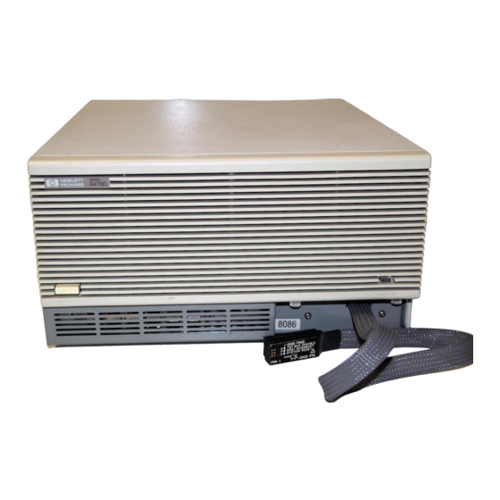
Figure 5-2. Attaching Grabbers to Probe Wires Connecting the The external analyzer probe is attached to a connector under the snap-on cover in the front upper right corner of the emulator. Probe to the Emulator Remove the snap-on cover by pressing the side tabs toward the center of the cover;...
Page 110: Figure 5-3. Removing Cover To Emulator Connector
Figure 5-3. Removing Cover to Emulator Connector Each end of the ribbon cable connector is keyed so that you can connect it to the emulator in only one way. Align the key of the ribbon cable connector with the slot in the emulator connector, and gently press the ribbon cable connector into the emulator connector (see figure 5-4).
Page 111: Figure 5-4. Connecting The Probe To The Emulator
Figure 5-4. Connecting the Probe to the Emulator Caution Turn OFF target system power before connecting analyzer probe wires to the target system. The probe grabbers are difficult to handle with precision, and it is extremely easy to short the pins of a chip (or other connectors which are close together) with the probe wire while trying to connect it.
Page 112: Connecting Probe Wires To The Target System
Connecting Probe You can connect the grabbers to pins, connectors, wires, etc., in the target system. Pull the hilt of the grabber towards the back of the Wires to the Target grabber handle to uncover the wire hook. When the wire hook is System around the desired pin or connector, release the hilt to allow the tension of the grabber spring to hold the connection (see figure...
Page 113: Configuring The External Analyzer
C onfiguring the After you have assembled the external analyzer probe and connected it to the emulator and target system, the next step is to External Analyzer configure the external analyzer. The external analyzer is a versatile instrument, and you can configure it to suit your needs.
Page 114: Should Emulation Control The External Bits
Should Emulation This configuration question allows you to specify whether the emulation interface should control the external analyzer. Control the External Bits? The default configuration selects "yes". You must answer "yes" to access the remaining external analyzer configuration questions. At the end of the configuration process the external analyzer mode and threshold voltages will be set;...
Page 115: Slave Clock Mode For External Bits? (State Mode Only)
The external analyzer may also operate as an independent state analyzer, or it may operate as an independent timing analyzer if a host computer interface program is used. emulation Selects the emulation mode (which is the default). In this mode, the external analyzer becomes an extension of the emulation analyzer.
Page 116: Figure 5-6. Mixed Clock Demultiplexing
mixed When the slave clock mode is "mixed", the lower eight external bits (0-7) are latched when the slave clock (as specified by your answers to the next four questions) is received. The upper eight bits and the latched lower eight are then clocked into the analyzer when the emulation clock is received (see figure 5-6).
Page 117: Figure 5-7. Slave Clocks
Figure 5-7. Slave Clocks demux When the slave clock mode is "demux", only the lower eight external channels (0-7) are used. The slave clock (as specified by your answers to the next four questions) latches these bits and the emulation clock samples the same channels again.
Page 118: Figure 5-8. True Demultiplexing
Figure 5-8. True Demultiplexing 5-12 Using the External Analyzer...
Page 119: Edges Of J (K,L,M) Clock Used For Slave Clock
Edges of J (K,L,M) clock used for slave clock? These four questions are asked when you select either the "mixed" or "demux" slave clock mode. They allow you to define the slave clock. You can specify rising, falling, both, or neither (none) edges of the J, K, L, and M clocks.
Page 120: Configuring Interactive Measurements
First external label polarity? This configuration question allows you to specify positive or negative logic for the external bits. In other words, positive means high= 1, low= 0. Negative means low= 1, high= 0. Define second external label? Allows you to define additional labels. Up to eight external labels can be defined.
Page 121: Using The Analyzer Trigger To Drive The External Analyzer
Interactive Measurement Specification BNC <-??-> ---\ BNC <-??-> ---\ CMBT <-??-> ---| CMBT <-??-> ---| | Trig1 | Trig2 Emulator <---------| Emulator <-??------| Analyzer ------> --/ Analyzer <-??-> --| External Analyzer <-??-> --/ NOTES: 1. The connections marked "??" are set up here in configuration. 2.
Page 122: Saving The Configuration
Refer to the chapter on "Coordinated Measurements" in the HP 64700-Series Emulators Softkey Interface Reference for more information on setting up interactive measurements. S aving the Save the changes to the configuration file either in a system defined file or in a user file of your choice. The system defined file is: Configuration /usr/hp64000/inst/emul/<...
Page 123: Timing: Introduction
Timing: Introduction O verview External timing commands are present in the firmware resident Terminal Interface. However, these commands output data in a binary format, and a host computer interface program is necessary to interpret and display the binary information. The Timing Analyzer Softkey Interface program is one such host computer interface.
Page 124: Measurement Modes
User-defined labels for the external probes signals. Store measurement data along with the system configuration. Comparison of stored and current measurements. Automatically mark user-specified events in trace data memory. Calculation of statistics on marked events. Support of graphics monitors as well as terminals (with an ASCII character waveform display).
Page 125: Glitch Capture Mode
Figure 6-1. Standard Data Acquisition Mode Glitch Capture Mode This is the same as the standard mode except that glitch information is also stored for each sample. A glitch is detected when there are two or more transitions on a signal between samples.
Page 126: Trace Memory
Figure 6-2. Glitch Capture Data Acquisition Mode Trace Memory Trace memory can store 1010 trace states if the standard mode is used or 505 states if the glitch capture mode is used. The Trace The trace specification allows you to define the trigger condition about which trace states are captured.
Page 127: The Timing Diagram
addition, a repetitive execution can be halted when a post processing event is found. The Timing Diagram The timing diagram presents the trace memory in a waveform display. The diagram will appear as a graphics diagram on high or medium resolution monitors, and as an ASCII character diagram on standard terminals.
Page 128 N otes 6-6 Timing: Introduction...
Page 129: Timing: Getting Started
Timing: Getting Started O verview This chapter describes: Prerequites for using the Timing Analyzer Softkey Interface. Entering the Timing Analyzer Softkey Interface. Making a simple measurement. Entering numerical values. P rerequisites for Before you can use the external timing analyzer, you must have already completed the following tasks: Using the Timing Analyzer Softkey...
Page 130: Installation
Softkey Interface $ emul700 em68k <RETURN> at the HP-UX prompt. This initializes the emulator and loads the configuration. If you have not already modified the configuration for the external analyzer, you should do so here. Refer to chapter 5 "Using the External Analyzer" for information on configuring the external analyzer.
Page 131: Making A Simple Timing Measurement
M aking a Simple A simple timing analyzer measurement can be made using the following sequence. Timing 1. Default the analyzer to an initialized condition. Measurement display format_specification <RETURN> default all_specifications <RETURN> 2. Set the threshold for the logic family which you desire to analyze.
Page 132 8. Move the cursor on the timing diagram by pressing the softkey CURSOR and then using the < leftarrow> and < rightarrow> to move the cursor. Note Use < CTRL> -F and < CTRL> -G along with < PREV> and <...
Page 133: Entering Numerical Values
E ntering As with the emulator Softkey Interface, you can enter numerical values in four standard bases: binary, decimal, octal, and Numerical Values hexadecimal. You must include the base letter after the number you enter, as follows: Binary (example: 10010110b). Q q O o Octal (example: 377o or 377q).
Page 134 N otes 7-6 Timing: Getting Started...
Page 135: Timing: Using The Analyzer
Timing: Using the Analyzer O verview This chapter shows you how to use the external timing analyzer. The main sections in this chapter describe how to: Move around the analyzer interface. Reference analyzer signals. Select measurement options. Specify the trigger condition. Start and stop a trace.
Page 136: Moving Around The Analyzer Interface
M oving Around The Timing Analyzer Softkey Interface uses eight screens to display analyzer information. Each screen has a set of associated the Analyzer functions. Some of the functions are common to all of the screens Interface and some of the functions are specific to a particular screen. The interface has three "specification"...
Page 137: Referencing Analyzer Signals
The command display trace_specification <RETURN> will display and set the Softkey labels for the trace specification options. R eferencing This section will describe how to specify threshold voltages for the probe signals, test for activity on the probe, and manage labels for Analyzer Signals each of the signals.
Page 138: Testing For Signal Activity
Note The threshold settings will not take effect until the next time you execute a trace or activity test. Testing for Signal After you have connected the probe grabbers to the points which have signals of interest, you can test for activity on the probe. The Activity command activity_test <RETURN>...
Page 139: Modifying Label Definitions
Note You should not confuse the default labels XBITS, X_lower, and X_upper with the probe signal groups xbits, x_lower, and x_upper. The command define CLK xbits_bit 0 logic_polarity positive_true <RETURN> gives probe signal "0" the label CLK and uses a positive polarity as logical true.
Page 140: Selecting Measurement Options
S electing The section describes how to select one of the two analyzer modes and the sample period or rate. Measurement Options Selecting the Timing The Timing Analyzer Softkey Interface has two modes: standard and glitch capture. Analyzer Mode Standard Mode The standard mode is the usual data acquisition mode.
Page 141: Selecting The Sample Period Or Rate
Selecting the Sample You can select the sample period (or rate, if it’s more convenient) with the "sample" command. Valid periods in the standard mode Period or Rate are between 10 ns (100 MHz) and 50 ms (20 Hz). Valid periods in the glitch capture mode are between 20 ns (50 MHz) and 50 ms (20 Hz).
Page 142: Trigger On Pattern Duration
specified, and the least significant bit is probe signal 0, or the least significant bit of the label specified. Refer to "Entering Numerical Values" in the previous chapter for valid pattern value options. The command trigger on pattern X_lower = 3AH <RETURN>...
Page 143: Less Than Duration
Less Than Duration The trigger occurs when the specified pattern is present on the probe signals for greater than 20 ns but less than the specified time duration. Durations from 40ns to 10 ms in 10 ns increments can be selected.
Page 144: Trigger Delay
Trigger Delay Trigger delay is the amount of time to delay the trigger after a valid trigger condition. Trigger delay can be anywhere between 0 and 10 ms in 10 ns increments. The command trigger 100 nsec_after pattern . . . <RETURN> sets the analyzer to trigger a trace 100 nanoseconds after a selected pattern condition is met.
Page 145: Execute
Note Refer to appendix D "Accurate Timing Measurements" for information on the statistical analysis of timing data. Execute The "execute" command starts a single trace. The trace is normally completed when the analyzer encounters the trigger condition. At that point trace memory is filled, the data is processed, and, finally, it is displayed, either in the timing diagram or the trace list form.
Page 146: Using The Timing Diagram
U sing the Timing This section describes the timing diagram and the features that allow you to change the display format. The timing diagram Diagram displays the currently in trace memory. Unless you are currently displaying the trace list, when you start a timing trace ("execute"), the timing diagram is automatically displayed.
Page 147 Signal Labels. The labels for the signals are displayed here. If the label refers to more than one probe signal, the logical bit number is added to the label display. If the signal refers to a label in a compare file, the signal reference is followed by an "x". You can change the signals displayed and the order they are displayed at any time.
Page 148: Presenting Signals
waveform display, the label drops down into the memory reference line in its relative location in trace memory. If more than one reference point is in the same location, an "m" is used to denote multiple references. The cursor is always in the display area, but is not labeled. In the lower magnifications, the cursor contains an optional horizontal set of bars.
Page 149: Moving The Cursor
The command present X_lower then blank then X_upper .0 <RETURN> presents all of the signals referred to by the default label X_lower, a blank line, and then the first signal in label X_upper (probe signal "8"). The command present <RETURN> toggles between user-defined labels and the corresponding probe signal labels.
Page 150: Showing Levels At The Cursor
The cursor can also be positioned by entering the relative sample number on the command line. The command <RETURN> moves the cursor to sample number one hundred, while the command <RETURN> positions the cursor at sample number minus fifty. In all cases, if the corresponding sample is not currently on the display, it will be centered in the display.
Page 151: Scrolling The Diagram
The command waveform_size large <RETURN> sets the waveform size to large. Scrolling the Diagram If you "magnify" the signal resolution or change the waveform size, all of the information may not fit in the waveform display area. The display area can then be thought of as a window on the whole waveform.
Page 152: Figure 8-2. Trace List Organization
sample number mode sample period statistical summary Trace List Timing (64700), 16 channels, 100MHz STANDARD MODE 10 nsec/sample Time x_o 6.00 usec Runs=0 Mean=0.0 nsec Stdv=0.0 nsec Label: X_upper X_lower XBITS time count Base: -0003 __01111111 10111110 0111111110111110 -30.0 nsec -0002 01111111 10111110...
Page 153 Mode. The mode for the current trace is displayed here. Sample Period. The sample period for the current trace is displayed here. Statistical Summary. The statistical summary displays the currently selected information. You can choose to display ("indicate") amount of time between the mark_x and mark_o points (interval statistics) or the number of occurrence marks (abcd) between the mark_x and mark_o points (occurrence statistics).
Page 154: Moving The Cursor
Using default label names, the command present X_lower then X_upper .0 <RETURN> displays the probe signals "0" through "8" in the display, grouped eight and one, and displayed as binary number, while the command present X_lower in_hex then X_upper in_hex then time_count absolute <RETURN>...
Page 155: Scrolling The Trace List
Scrolling the Trace The trace list display area can then be thought of as a window on trace memory. The window can be scrolled up and down. List The Shift-^ (Shift-< uparrow> ) and Shift-v (Shift-< downarrow> ) keys move the display up and down one line for each keystroke.
Page 156 You can search for a specific signal pattern with a command like find entering X_lower =01010111 <RETURN> that looks for specific combination of true an false signals on probe bits "0" through "7", or for a transition specific signal with a command like find entering X_lower .2 = 1 <RETURN>...
Page 157: Marking Events
You can designate a search pattern must last for a specified duration; it can be less than or greater than a selected amount of time. The command find greater_than 100 nsec_of X_lower .2 = 1 thru 600 <RETURN> searches for at least one hundred nanoseconds of a high signal on bit 2 of X_lower from the cursor to sample number 600.
Page 158 The syntax for the "mark" command is very much like that for the "find" command. The command mark x on_first_occurrence_of entering X_lower =01010111 <RETURN> places mark_x on the first occurrence of the pattern 01010111B on X_lower in trace memory while the command mark x on_first_occurrence_of entering X_lower .2 <RETURN>...
Page 159: Processing For Data
Processing for Data The "process_for_data" command is a way to limit the samples displayed on the trace list. As with the "find" and "mark" commands, a simple or complex set of conditions can be specified. You can display only samples that have been previously marked, specified new conditions for the display, or display samples a set number of samples after a new condition.
Page 160: Statistics
Statistics The Timing Analysis Softkey Interface can perform statistical analyses on repetitive executions traces. Two types of analysis are available: interval statistics and occurrence statistics. For both types of analysis, you can calculate the minimum and maximum values, or the mean and standard deviations. Choosing Statistics Types Interval Statistics Interval statistics are based on the time interval between mark_x and mark_o samples.
Page 161: Logging Statistics
marks from mark_x to mark_o is greater than (or less than) a specified number of marks. Logging Statistics You can log the detail from each sample to a file for subsequent review. The "statistics"‘ command in the post processing specification allows you to specify a file name to write the information.
Page 162: Comparing Current And Stored Measurements
C omparing The Timing Analyzer Softkey Interface allows you to store trace memory measurements in a file and then compare the stored data Current and to a subsequent trace measurement. Stored Measurements Storing In order to properly compare a saved trace measurement, its data is stored with all the specification (configuration) information.
Page 163: Presenting Stored Signals
The trigger position must be the same or a "Compare file spec does not agree with hardware" error will occur. Presenting Stored Once a compare file is selected, the signals from the previous trace can be presented, just as the current labels can be presented, on Signals either the timing diagram or the trace list.
Page 164: Copying Specifications
C opy Analyzer The Timing Analyzer Softkey Interface can copy all or part of its information to a file or to a printer, or "pipe" it to a HP-UX Data process. Refer to appendix B "Timing Output and Diagrams" for information on setting up the system printer environment.
Page 165: Copying Trace Data
These commands only work on the HP 9000 Series 300/400 computer. If you are using an HP 9000 Series 700 or Sun SPARCsystem computer running the X Window System, you can use the UNIX xwd and xpr commands to print the contents of the timing analyzer window.
Page 166: Copying Measurement Data
Copying The Timing Analyzer can also create a file containing "raw" trace memory data in hexadecimal format. This file can be used for other Measurement Data analysis. The command copy measurement_data_in_hex to TIMING_DUMP <RETURN> copies the current trace memory data to a file named TIMING_DUMP in hexadecimal format.
Page 167: Ending To Continue Later
In order to use the system again, you must reinitialize the analyzer configuration. Ending to Continue You can continue later without effecting other users by simply using the command Later end <RETURN> which ends the current session, but preserves the configuration status.
Page 168 N otes 8-34 Timing: Using the Analyzer...
Page 169: Timing : Commands
Timing : Commands O verview This chapter includes: Softkey Interface Features Syntax Conventions A Summary of Commands Command Descriptions S oftkey Interface Features Softkeys Softkey Interface commands are entered by pressing softkeys whose labels appear at the bottom of the screen. Softkeys provide for quick command entry, and minimize the possibility of errors.
Page 170: Command Line Recall
"cd" command. This command does not appear on the softkey labels. Filters and Pipes You can specify HP-UX filters and pipes as the destination for information while using the "copy" command. See the description of the "copy" command in this chapter for details.
Page 171: Help Command
Help Command A "help" command is available to you within an emulation session. Several methods are available for displaying help information about a command. You can use any of these methods: enter: help then press a softkey that appears enter: ? then press a softkey that appears enter: pod_commands this will return help from the emulator...
Page 172: Summary Of Commands
The commands available on each screen are outlined in table 9-2. The following commands can be entered at the command line on all screens: !HP-UX_COMMAND, cd, diagram, format, help, list, log_commands, pod, trace, and wait. Table 9-1. Summary of Commands...
Page 173 Table 9-2. Command Assignments Commands activity_test compare configuration copy CURSOR default define delete display execute find halt halt_repetitive_execution indicate magnify mark mode_is modify pod_command present process_for_data rename < ROLL> sample statistics threshold trigger waveform_size Timing: Commands 9-5...
Page 174: Command Syntax
C ommand Syntax The syntax for the HP 64700 external timing analyzer varies considerably from that used in the HP 64700-Series emulators. Therefore, the complete timing analyzer syntax is presented here. In certain cases, you may want to refer to your Emulator Softkey Interface User’s Guide or the HP 64700-Series Emulators Softkey...
Page 175: Activity_Test
a ctivity_test This command toggles the display of probe signal activity. Syntax Function This is a format specification command that displays the activity on the external analyzer probe. If the activity_test is currently being displayed, this command turns the activity_test display off. The activity line appears at the top of the label list.
Page 176: Compare
c ompare This command specifies a post processing compare definition. Syntax 9-8 Timing: Commands...
Page 177 Function This post process specification command is used to select a compare file or to specify a comparison to be performed after each measurement. Default Values none Parameters < BIT# > This prompts you to enter the integer bit number to be used. consecutive_faults_ This option allows you to define the number allowed_is...
Page 178 cursor This parameter specifies the cursor location as the beginning point of the comparison. start This parameter specifies the start of trace memory as the beginning point of the comparison. This parameter specifies the end of trace memory as the beginning point of the comparison.
Page 179 Examples display post_process_specification <RETURN> compare file_is FIRST_TRACE <RETURN> Related Commands configuration present Timing: Commands 9-11...
Page 180: Configuration
c onfiguration This command creates or retrieves a configuration file. Syntax Function The configuration command allow you to save configurations or to load a previously saved file to reset specifications. Measurement data may also be saved with the configuration information. In that case, the configuration can be used as a compare file.
Page 181 create a file for use with the compare command. write_protect This parameter sets the write protect variable in the file descriptor. Examples configuration save_in FIRST_TRACE with_data <RETURN> Related Commands compare Timing: Commands 9-13...
Page 182: Copy
c opy This command copies specifications, displays or measurement data to selected output. Syntax 9-14 Timing: Commands...
Page 183 Function The copy command allows you to copy the all or selected specifications, displays or lists, statistics, help, or measurement data to a file, printer or HP-UX command. Note < CTRL> -C (SIGINT) will interrupt a copy command. Default Values...
Page 184 This option copies the timing diagram to the selected output. The default format is in "raw" HP PCL format. vertically_in_ascii This parameter specifies the timing diagram output to be in ASCII characters oriented vertically on the page. That is rotated clockwise ninety degrees from its normal orientation.
Page 185 < SAMPLE> This prompts for you to enter a sample number. Trace memory data between the cursor and the entered sample number will be copied. start This parameter specifies that trace memory data between the start of memory and the cursor will be copied.
Page 186 This option initiates the selection of a destination for the specified data. Examples copy measurement_data_in_hex to HEXDUMP <RETURN> copy display to printer <RETURN> copy all_specifications to specfile<RETURN> Related Commands none 9-18 Timing: Commands...
Page 187: Cursor
C URSOR This command toggles the use of the cursor keys from the command line to the timing diagram. Syntax None Function When the CURSOR softkey appears without the asterisk, the right and left arrow keys are available for command line editing. When the CURSOR softkey appears with an asterisk (CURSOR*), you can move the cursor in the timing diagram display with the right and left arrow.
Page 188: Default
d efault This command sets specifications to their default values. Syntax Function The default specifications can be set for the trace or post process specifications or for all specifications. Default Values none Parameters all_specifications This option sets the trace, format, and post process specifications to their default values.
Page 189: Define
d efine This command creates a label which is used to refer to probe signals. Syntax Function This is a format specification command that creates a new label and associates one or more probe signals to the label. Logic polarity can also be designated. An existing label definition can be modified using this command.
Page 190 < LABEL> This prompts you for the name of an existing label either entered or selected from a softkey. xbits_bit This is a syntactical item referring to the external probe signal bits. < BIT# > This prompts you to enter the starting bit number.
Page 191 define DATA xbits 8 width 8 <RETURN> Related Commands delete rename threshold Timing: Commands 9-23...
Page 192: Delete
d elete This command deletes one or all labels. Syntax Function This format specification command deletes one or more labels. If a label is used in another specification, an error message will inform you it cannot be deleted. If a deleted label has been reference in the timing diagram or trace list, it is automatically removed from the display.
Page 193: Diagram
d iagram This command initiates the timing diagram softkeys. Syntax none Function This command invokes the "diagram" softkeys from whatever "display" mode you are currently in. This allows you to enter timing_diagram specific commands without the necessity of using "display" to change specification modes. Default Values none Parameters...
Page 194: Display
d isplay This command selects the screen to display. Syntax Function The display commands moves between the three specification screens and the two output screens. Three special function screens can also be displayed: pod commands, error log, and event log. Entering any of the words trace, format, pod, post, diagram, and list will allow the commands from that specification or output screen to be accessible.
Page 195 trigger the timing analyzer to begin acquiring data. format_specification This option selects the format specification where you can define labels and set thresholds which the analyzer will use. post_process_ This option selects the post processing specification specification where you can define events to be completed after every execution.
Page 196: End
e nd This command terminates the analyzer session. Syntax Function This command terminates the current timing session. If you end or end locked, you keep the analyzer in a locked state. In addition, end locked terminates the any other sessions running on the analyzer in other windows or on other terminals.
Page 197 You return to the HP-UX shell or PMON depending on how you entered emulation. Unless you choose "end release_system", the current emulation configuration is stored so that on reentry to the emulation module, you can resume the emulation session. Note Entering <...
Page 198 Softkey Interface was entered. In addition, the emulator is unlocked so that it may be used by other users on your HP-UX system. The information needed to continue your session is also removed. (If you do not release the system, no other users may access it.)
Page 199: Execute
e xecute This command starts one or more timing measurements. Syntax Function The timing analyzer can make both single module or multiple module measurements by using the execute and halt commands. The execute command will start the timing analyzer alone (single module measurement) if the timing analyzer is not connected to the intermodule bus (IMB).
Page 200 Examples execute repetitively <RETURN> Related Commands halt halt_repetitive_execution 9-32 Timing: Commands...
Page 201: Find
f ind This command finds a trigger-like event in trace memory. Syntax Timing: Commands 9-33...
Page 202 Function This command locates the specified event in trace memory and brings it into the display, centers it, if possible, and locates the cursor at that point. You can use this command to locate the trigger, any of the marked samples, or specified signal conditions on a label, multiple labels or a combination of label bits.
Page 203 specified pattern for more than the selected duration within the specified range. < LABEL> This prompts you to enter a label name or select the label name from the softkeys. leaving This option locates the object label, labels, or combinations of label bits leaving the specified pattern within the specified range.
Page 204 thru This parameter selects a range in trace memory to search. The first point is the cursor position. The second point is a selected parameter. trigger This parameter specifies that trace memory data between the cursor and the trigger will be searched.
Page 205 This option specifies the label, labels, or combination of label bits in the "any_transition" and "any_glitch" options. or_on This option further specifies the objects referred to in the "on" option. This option further specifies the objects referred to in the entering, leaving, greater_than, or less_than options.
Page 206: Format
f ormat This command initiates the format specification softkeys. Syntax none Function This command invokes the "format" softkeys from whatever "display" mode you are currently in. This allows you to enter format specification specific commands without the necessity of using "display"...
Page 207: Halt
h alt This command terminates the execution in process. Syntax Function The halt command will terminate the current measurement and display the last segment of captured data before the halt command was entered. This command is only available while executing measurements and is most useful to halt a repetitive execution.
Page 208 h alt_repetitive_exec This command conditionally halts a repetitive execution. ution Syntax Function This post processing command terminates a repetitive execution if the conditions specified in the command are met. Conditions include numbers of runs, specified sequences of marks, specified mark counts, or when the time between mark_x and mark_o is more or less than a certain value.
Page 209 Default Values A repetitive execution will continue until halted by command or post processing conditions are specified. Parameters modify This option returns the current halt_repetitive_execution command to the command line for editing. when_marks_x_o This option specifies a count of the marks (a,b,c,d) between the mark_x and mark_o as the condition to halt a repetitive execution.
Page 210 mark_a, One of these parameters is selected as a mark_b, condition. mark_c, mark_d, any_mark then This parameter allows you to include an additional condition in a sequence. then_not This parameter allows you to exclude a condition from a sequence. when_time_x_o This option specifies a mark_x to mark_o duration as the condition for halting a repetitive execution.
Page 211 Examples halt_repetitive_execution when_time_x_o greater_than 100 nsec <RETURN> halt_repetitive_execution when_sequence_x_o mark_a then mark_b then_not mark_c <RETURN> Related Commands execute halt Timing: Commands 9-43...
Page 212: Help
h elp This command allows you to display information about the system and analyzer features during an analyzer session. Syntax Function Typing "help" or "?" causes the available help options to be displayed on the softkey labels. The system will display the help information on the screen when you select an option.
Page 213 This is a summary of the commands that appear on the softkey labels when you type "help" or press "?": system_commands simple_measurement_commands trace_specification_commands format_specification_commands post_process_specification_commands display_commands execute_commands diagram_commands list_commands configuration_commands copy_commands graphic_diagrams ascii_diagrams diagram_outputs end_commands Related Commands none Timing: Commands 9-45...
Page 214: Indicate
i ndicate This command selects the statistical information displayed. Syntax Function This command allows you to select display information. The display information can be either the time between mark_x and mark_o or the number of marks (a, b, c, d) between mark_x and mark_o.
Page 215 maximum_and_ This parameter specifies the maximum and minimum minimum values for the selected display option are to be displayed. mean_and_ This parameter specifies the mean and standard_deviation standard deviation for the selected display option are to be displayed. levels_at_cursor This option selects the display of signal levels at the diagram cursor on the timing diagram.
Page 216: List
l ist This command initiates the trace list softkeys. Syntax None Function This command invokes the "list" softkeys from whatever "display" mode you are currently in. This allows you to enter trace list specific commands without the necessity of using "display" to change specification modes.
Page 217: Magnify
m agnify This command changes the timing diagram display resolution. Syntax Function This timing diagram command allows you to change the time per division specification in the timing diagram display. This allows you to observe the signals in greater or lesser detail. It also allows you to turn the indicator bar on or off.
Page 218 Parameters Choose one of these options to set the magnification to a factor of 1, 2, 4, 10, 20, 40, or 100, respectively. The time per division x10, information on the screen changes x20, accordingly, along with the magnification x40, value field.
Page 219: Mark
m ark This command marks specified conditions in trace memory. Syntax Timing: Commands 9-51...
Page 220 Function Marks are identifiers assigned to samples in trace memory. They can be assigned to any "event" you specify. Marks can be assigned from the command line for events in current trace memory, or as a post processing function. Marks specified at the command line are also store for subsequent post processing.
Page 221 Specify conditions for halting repetitive executions. There six mark names recognized: mark_x, mark_o, mark_a, mark_b, mark_c, and mark_d. The first two marks, mark_x and mark_o, are single occurrence marks and are used to identify the first occurrence of a specified event. These two marks always exist and are used to define a range of samples.
Page 222 or_on This parameter allow you to add an additional glitch condition label name or label bit number. any_transition This parameter qualifies the transition condition by specifying a label name or label bit number. or_on This parameter allow you to add an additional transition condition label name or label bit number.
Page 223 greater_than This option specifies a pattern will exist for more than an specified duration. < LABEL> This prompts you to enter a label name or select the label name from the softkeys. leaving This option specifies a pattern condition will be exited.
Page 224 on_sample This option specifies the mark is to be moved to the specified trace memory sample number. on_trigger This option specifies the mark is to be moved to the current trigger location. < PATT> This prompts you to enter a pattern of signals.
Page 225 Examples mark x on_first_occurrence_of entering XBITS = 0B0H <RETURN> mark a on_all_occurrences_of any_transition after mark_x <RETURN> mark d on <RETURN> mark c on_all_occurrences_of entering XBITS .1 = 0 named EVENT <RETURN> Related Commands find Timing: Commands 9-57...
Page 226: Mode_Is
m ode_is This command sets the data acquisition mode. Syntax Function This command sets mode to either "standard" or "glitch_capture". In the standard mode, trace memory can hold 1024 samples taken at the rate specified. In the glitch_capture mode, trace memory can hold 512 samples and glitchs are noted.
Page 227: Modify
m odify This command returns the define label command for editing. Syntax Function This format specification command allows you to modify the definition of any existing label. Default Values none Parameters < LABEL> This prompts you to enter a label name or select the label name from the softkeys.
Page 228: Pod
p od This command initiates the pod commands softkeys. Syntax None Function This command invokes the "pod_commands" softkeys from whatever "display" mode you are currently in. This allows you to enter pod_command specific commands without the necessity of using "display" to change specification modes. Default Values none Parameters...
Page 229: Pod_Command
p od_command This command sends native commands to the analyzer. Syntax Function This command sends native commands to the analyzer terminal interface. You should be very careful to avoid command which will effect the interface or the configuration. Those commands would "confuse"...
Page 230 Parameters < CMD> This prompts you to enter a quoted sting literal to send to the analyzer firmware. The contents of the quoted string are sent and the results are displayed on the screen. Examples pod_command "ver" <RETURN> Related Commands none 9-62 Timing: Commands...
Page 231: Post
p ost This command initiates post_process specification softkeys. Syntax none Function This command invokes the "post_process" softkeys from whatever "display" mode you are currently in. This allows you to enter post process specific commands without the necessity of using "display" to change specification modes.
Page 232: Present
p resent This command specifies the objects to be presented. Syntax The timing diagram syntax is: The trace list syntax is: 9-64 Timing: Commands...
Page 233 Function This command controls the display format for the timing diagram and trace list. The timing diagram display can include all defined labels or any combination of blank lines, labels or label bits, or compare file labels or label bits (if the compare file has been selected).
Page 234 between default and user-defined labels on the timing diagram. < DOT> This prompts you to enter the literal "." to designate a specific bit number for a label. in_hex, Specifies the number base when the trace list in_oct, is being shown. The bases are hexadecimal, in_bin, octal, binary, and decimal, respectively.
Page 235 Examples present TIMER then DATA .0 thru 3 then blank then DATA .4 thru 7 <RETURN> present DATA then blank then compare_file DATA <RETURN> present mark_names then TIMER in_bin then DATA in_hex then time_count relative <RETURN> Related Commands define Timing: Commands 9-67...
Page 236: Process_For_Data
p rocess_for_data This command limits the trace list display to specified samples. Syntax 9-68 Timing: Commands...
Page 237 Function This trace list command limits the samples displayed to those from trace memory that meet the specified conditions. Conditions can include samples with a specified pattern, samples a fixed count from specified transition, only marked samples, or samples with a specified pattern lasting more than a specific time period.
Page 238 This option turns the process for data condition off. When there is no process for data condition, all of the samples in trace memory are displayed in the trace list. This parameter qualifies the transition condition by specifying a label name or label bit number.
Page 239 pos_transition_on This parameter specifies a positive transition on the target signal. pos_or_neg_ This parameter specifies any transition on transition_on the target signal. < TIME> This prompts you for the time period to look for a specified pattern. nsec, These parameters specify the units of usec, measurement of <...
Page 240: Qualifier
Q UALIFIER The QUALIFIER parameter is used with the "trigger" command to specify a conditions after which a trigger condition will be tested. Syntax 9-72 Timing: Commands...
Page 241 Function You can specify a condition or set of conditions that must be met before the trigger condition will be evaluated. In standard mode, qualifiers on "edges", or changes in signal values, while in glitch capture mode, qualifiers are glitches. Default Values There is no default for qualifying standard mode triggers.
Page 242 occurred. If you specify one or more signals, the trigger will be qualified by glitches only on those lines. Otherwise, glitches on any line will cause the qualification to be true. Examples trigger on pattern XBITS .0 = 0 qualified_with positive_edge XBITS .1 <RETURN>...
Page 243: Rename
r ename This command renames a defined label. Syntax Function This format specification command renames any previously defined to another name. Default Values none Parameters This option initiates the entry of the new name for the label. < LABEL> This prompts you to enter a label name or select the label name from the softkeys.
Page 244: Roll
< ROLL> This softkey describes how to move around the timing diagram. Syntax none Function The < ROLL> softkey reminds you that you can enter a sample number, or use the < CTRL> -F and < CTRL> -G (or < NEXT> and <...
Page 245 Scrolls the diagram down by one line if all of < downarrow> the displayed signals do not fit on one screen. < Shift> -^ Scrolls the diagram up by one screen if all of < Shift> -< uparrow> the displayed signals do not fit on one screen. <...
Page 246: Sample
s ample This command specifies the sampling period or rate. Syntax Function The sample command sets the sampling period or rate for subsequent measurements. Data is acquired by the analyzer and stored in trace memory at that effective rate. Default Values The default is the fastest sample rate in each mode.
Page 247 rate_is This option specifies the sample rate based on the frequency if sampling. < FREQ> This prompts you to enter the sample frequency. The allowed range is 100 megahertz (50 megahertz in glitch_capture mode) to 2 hertz. MHz, These parameters specify the units of kHz, measurement of <...
Page 248: Statistics
s tatistics This command selects samples to be included in statistical analysis. Syntax Function This command specifies samples on which statistics are to be calculated. Samples are qualified with mark counts or time intervals from mark_x to mark_o. This command can also log the statistics after every execution to a specified file.
Page 249 Parameters always This option resets this option to its default condition. when_marks_x_o This option specifies that only traces with a number of marks between the mark_x and mark_o points (inclusive) will be included in the statistical sample. greater_than This parameter specifies the mark count must be greater than the number entered.
Page 250 log_to_file The option selects a file name to receive statistical information. < FILE> This prompts you for a file name to contain the output information. noappend This parameter forces the overwrite of a file’s information if the selected file name already exists.
Page 251: Threshold
t hreshold This command sets the point at which a signal voltage is considered a logical true. Syntax Function This command sets the voltage level at which a signal is considered true (a logical "1") for each of the two signal groups, or for all signals.
Page 252 This parameter sets the threshold voltage to + 1.40V. This parameter sets the threshold voltage to -1.30V. cmos This parameter sets the threshold voltage to + 2.50V. < VOLTS> This prompts you to enter the voltage if it is non-standard. volts This is a syntactic element used when entering the voltage.
Page 253: Trace
t race This command initiates the trace specification softkeys. Syntax none Function This command invokes the "trace" softkeys from whatever "display" mode you are currently in. This allows you to enter trace specification specific commands without the necessity of using "display"...
Page 254: Trigger
t rigger This command specifies trigger conditions. Syntax 9-86 Timing: Commands...
Page 255 Function The trigger is an event on the probe which causes the analyzer to begin acquiring data and filling trace memory. The trigger command can also position the trigger at the start, center, or end of trace memory. Default Values The default is a "don’t care"...
Page 256 nanoseconds, microseconds, or milliseconds, respectively. < DOT> This prompts you to enter the literal "." to designate a specific bit number of a label. greater_than This option specifies a duration a pattern should last for the specified signals. If the pattern is detected but does not last at least the specified amount of time, the trigger condition is not met.
Page 257 the samples will be evenly distributed on either side of the trigger. start_of_trace This parameter positions the trigger near the start of trace memory. center_of_trace This parameter positions the trigger near the middle of trace memory. end_of_trace This parameter positions the trigger near the end of trace memory.
Page 258: Wait
w ait This command allows you to present delays to the system. Syntax Function The wait command can be an enhancement to a command file, or to normal operation at the main analyzer level. The usefulness of delays is to allow the analyzer system and external analyzer time to reach a certain condition or state before executing the next command.
Page 259 Parameters measurement_ This option causes the system to pause until complete a pending measurement completes, or until a < CTRL> -C signal is received. If a measurement is not in progress, the wait command will be completed immediately. This causes the system to wait for a <...
Page 260: Waveform_Size
w aveform_size This command adjust the waveform size on the display. Syntax Function This timing diagram command allows you to adjust the size of the displayed waveforms. A small waveform size allows you to compare waveforms of a greater number of signals. A large waveform size allows you to view the signal in more detail.
Page 261 Examples display timing_diagram <RETURN> waveform_size medium <RETURN> Related Commands present Timing: Commands 9-93...
Page 262 N otes 9-94 Timing: Commands...
Page 263: External Analyzer Specifications
External Analyzer Specifications General Threshold Accuracy = + /- 50 mV. Specifications Threshold Voltage Range = -6.40V to 6.35V. Dynamic Range = + /- 10 V about threshold setting. Minimum Input Swing = 600 mV pp. Minimum Input Overdrive = 250 mV or 30% of threshold setting, whichever is greater.
Page 264: Timing Analyzer
Minimum Clock Width = 10 ns. Minimum Clock Period: – No Tagging Mode = 40 ns (25 Mhz clock). – Event Tagging Mode = 50 ns (20 MHz clock). – Time Tagging Mode = 60 ns (16 MHz clock). Minimum Time from Slave Clock to Master Clock = 10 ns. Minimum Time from Master Clock to Slave Clock = 50 ns.
Page 265: Timing Output And Diagrams
Timing Output and Diagrams O verview The Timing Analyzer Softkey Interface provides you a mechanism to generate output for a variety of environments and hardware. Measurements can be displayed in diagrammatic or list form. Diagrams are created using ASCII characters, the default, for ASCII terminals and non-graphics printers, or in graphics format for terminals and printers with graphics support.
Page 266: Graphics Timing Diagrams
Graphic timing diagrams are available when using the X Window System on a bit-mapped display, but are not available when running HP Windows/9000 on a bit-mapped display, or on an ASCII terminal. Graphic timing diagrams are available on a remote SPU only with the X Window System.
Page 267: Wmscrn Shell Variable
Video Board. hp98700 HP 98700H Graphics Display Station. hp98720w HP 98720H / HP 98721 Graphics Display Stations. WMSCRN Shell Now when you enter the timing analyzer and press "execute" a graphics timing diagram should appear. If graphics do not appear...
Page 268: Required Filesets
The fileset AFA_FM, which contains raster fonts for graphics and text, is required for the timing analyzer to produce graphic displays. See the HP-UX System Administrator Manual, Part 2 for information on loading the required filesets. U sing the Timing The graphic timing diagram is available under the X Window System Version 11.
Page 269: Windowid Shell Variable
For information on using the Timing Analyzer connected to a remote host, refer to "Remote Connections" later in this section. WINDOWID Shell The timing analyzer looks for the shell variable WINDOWID to determine the windowid of the terminal emulator window which Variable the timing analyzer is running in.
Page 270 reverseVideo Specifies that the foreground and background colors should be reversed. timingGeometry Specifies the location and size to create the timing analyzer’s graphics subwindow. This X default should not be used unless the timing analyzer is positioning and/or sizing it’s graphics subwindow incorrectly. This can occur if the terminal emulator window is created with an unusually large internal border or a left-justified scroll bar is being...
Page 271: Remote Connections
".rhost" file on the remote host. You should refer to the "Customizing Your Local X Environment" in Using the X Window System: HP 9000 Series 300/800 Computers for more information on using remote hosts. Timing Diagrams and Outputs B-7...
Page 272: Ascii Timing Diagrams
Once this environment has been configured, an "hpterm" window can be opened for the timing analyzer on the remote host with the command: remsh timingnode -n "DISPLAY=mynode:0.0 /usr/bin/X11/hpterm" & <RETURN> where: timingnode is the remote host name, and mynode is the local host name. The remote host will open an "hpterm"...
Page 273: Customizing The Ascii Diagram
These four types of input are loosely delimited by the colon character ":". Note The first three colon ":" characters in the example above are ASCII characters used to represent the glitch capture mode in large, medium and small waveforms, respectively. Customizing the ASCII Diagram Waveform Sizes and ASCII Characters...
Page 274: Row Locations For Mark Indicators
Where "g" represents the one character to be displayed for a low, high, glitch, and middle level in the small waveform. As examples, the default diagram is: For a low "g" = "_". For a high "g" = "*". For a glitch "g"...
Page 275: Characters To Define The Cursor
c_st_l is the cursor starting row for large waveform c_int_l is the cursor interval row for large waveform c_st_s is the cursor starting row for small waveform c_int_s is the cursor interval row for small waveform Acceptable values for all variables are integers between "0" and "15". A "c_st_l"...
Page 276: Printer Requirements
P rinter The graphic timing diagram outputs can be saved in files or sent to a laser (HP LaserJet) printer, or an equivalent, as well as a Requirements dot-matrix printer which supports raw raster dumps. The timing analyzer needs two printer shell variables setup to function properly PRINTER and GPRINTER.
Page 277: Using Measurement Data In Hexadecimal
U sing You can store raw measurement data in a ASCII file in hexidecimal format by using the "copy measurement_data_in_hex to < FILE> " Measurement command. This file can be used for further analysis or comparison. Data in Hexadecimal Understanding the The measurement data output is a list of all the data samples in trace memory stored from first to last.
Page 278: Glitch Capture Mode Data Format
A "1" in a bit indicates the data sample is high. A "0" in a bit indicates the data sample is low. Glitch Capture Mode In the glitch capture mode, the data sample represent the values: Data Format Bit0 = xbit0 data Bit1 = xbit1 data Bit2 = xbit2 data Bit3 = xbit3 data...
Page 279: Comparing Measurement Data To A Trace List
Comparing To illustrate the relationship between the raw measurement data file and the trace memory samples, review at the two listings below. Measurement Data to The first listing a the first portion of a measurement data file. a Trace List 64700 Timing Analyzer Fri Jun 9 11:00:59 1989...
Page 280 N otes B-16 Timing Diagrams and Outputs...
Page 281: Timing Messages
Timing Messages O verview Three types of messages appear in the analyzer message line: status messages, informational messages, and error messages. The message text along with an explanation and possible responses are detailed later. A measurement status message also appears on the right hand side of the status line.
Page 282 STATUS: External analysis not configured for timing This message appears when the configuration file loaded into the emulator/analyzer has not been configured for external timing analysis. The following message also appears: The configuration file loaded has not configured the external analyzer for Timing measurements.
Page 283: Informational Messages
STATUS: Marking complete, found xxx marks (abcd) This message indicates marking has been completed in the post processing. The xxx represents the total number of marks found for all mark names (mark_a, mark_b, mark_c, and mark_d). STATUS: Marking complete, marking limit of 511 exceeded This message indicates marking has been completed in the post processing and more than 511 events meet the conditions for marking (abcd).
Page 284: External Trace Complete
"External trace complete" Trigger event was found and trace is complete. "External trace halted" The last trace was halted. ENTER: ’Return’ to place the mark at the current cursor location This message appears when entering the < MARK> softkey under the "mark x"...
Page 285 ERROR: Compare definition is invalid This message is displayed then you redefine labels in such a way that the compare definition is no longer valid. The compare definition will need to be recreated. ERROR: Compare file is invalid, compare file is removed This message indicates that a compare file has been modified and is no longer recognized as a compare file.
Page 286 ERROR: Configuration load failure This message appears when the configuration file could not be loaded due to an interrupt or other HP-UX system problem. You identify the problem and try to reload the configuration file. ERROR: Data is not present in hardware This message appears when you try to save a configuration file "with_data"...
Page 287 ERROR: Duration is greater than trace memory This message indicates you have entered a duration that is greater than the duration of the entire trace memory. You need to enter a valid duration or change the sample period to extend the trace memory duration length.
Page 288 ERROR: Halt_repetitive_execution definition is invalid This message is displayed when you change the mode or redefine the sample period is such a way that the halt_repetitive_execution condition is not longer valid. You need to correct the halt_repetitive_execution condition. ERROR: Help keys are not defined properly This message indicates the timing analyzer help keys have been incorrectly defined.
Page 289 mode. You need to correct the trigger specification or change modes. ERROR: New label already exists This message appears when trying to rename a format specification label to a new name. The new name already exits and cannot be reused without removing the existing name. The existing name can itself be renamed or deleted.
Page 290 ERROR: Sample rate is too slow for sampled trigger duration This message is displayed when you try to enter a combinational glitch trigger definition where the sample period is longer than the trigger duration. Glitch triggering requires all data to be sampled before trigger duration detection circuitry, and thus requires the sample period to be less than one-half the specified duration.
Page 291 ERROR: Timing graphics initialization failed This message appears when the timing analyzer is unable to use graphics for displaying the timing diagram; the ASCII diagram format will be used. Refer to appendix C "Timing Output and Diagrams" for information on setting up a graphics environment. Timing Messages C-11...
Page 292 N otes C-12 Timing Messages...
Page 293: Accurate Timing Measurements
Accurate Timing Measurements I ntroduction This appendix provides information for making accurate time interval measurements with the timing analyzer. Accurate time interval measurements depend primarily on the time interval resolution of the timing analyzer. If you have a good time interval resolution, using statistics can improve the accuracy of a measured time interval by the amount described in the equations which you will find in this appendix.
Page 294: Factors
Factors Sample Period The sample period is the amount of time between samples. Interchannel Skew Interchannel skew is the difference in delays of the probe channels, including delay differences from one channel to another, and delay differences in recognizing negative and positive transitions. Skew is a function of several input variables as follows: Input signal slew rate in volts/ns (low slew rate increases the skew).
Page 295: Calculation
To measure longer intervals, the sample period must be increased. Calculation Resolution is formally defined as: resolution = + /- (sample period + skew). A high sample rate (100 MHz), coupled with low skew (plus or minus 4 ns for both opposite and same direction transitions), gives the timing analyzer very good resolution.
Page 296: Improving The Accuracy Of Mean Value Measurements
Note The time interval being measured must not be synchronous to the sampling clock of the timing analyzer. Typically, this is not a problem in the timing analyzer unless the sample rate is extremely low. The timing analyzer halts its interval sample clock between each measurement;...
Page 297: Accuracy Of Standard Deviation Measurements
A ccuracy of An interval that does not vary still can be shown to have a large standard deviation due to the sampling process. The error in the Standard displayed standard deviation depends on the size of two elements: Deviation Measurements the portion of the interval that exceeds the multiple of the sample periods;...
Page 298: Statistical Errors Caused By Sampling Process
S tatistical Errors The timing analyzer calculates statistics on the sampled data in its memory, not on all of the data generated by the system under test. Caused by The data in memory may misrepresent the actual data. Misleading Sampling Process data can be captured when you trigger your trace on some occurrence that causes the timing analyzer to capture samples at misleading points in the data flow of a system under test.
Page 299 Index about, trigger position specification, 2-10 absolute files, loading, 2-6 absolute, displaying count information, 3-12 absolute, trace display option, 3-6 activity measurements (SPMT), 4-2 additional symbols for address, 4-13 confidence level, 4-14 error tolerance, 4-14 example, 4-21 interpreting reports, 4-12 mean, 4-13 relative and absolute counts, 4-14 standard deviation, 4-13...
Page 300 analyzer probe assembling, 5-2 connecting to the emulator, 5-3 connecting to the target system, 5-5 bases (number), 2-9 before, trigger position specification, 2-10 binary numbers, 2-9, 7-5 blank, 9-65 break on guarded memory access, 2-30 cautions check for bent pins when connecting analyzer probe, 5-3 turn off target before connecting analyzer probe, 5-5 change directory, 9-2 clocks...
Page 301 copy (continued) trace data, 8-31 count absolute/relative, trace display option, 3-12 count information in trace listing, 2-7 count qualifier, 1-1 count qualifiers, 2-18 count, occurrence, 2-19 cursor, 9-19 moving in timing diagram, 8-15 moving in trace list, 8-20 data (external), trace display option, 3-15 data qualifiers, 2-21 decimal numbers, 2-9, 7-5 default, 9-20...
Page 302 display trace (continued) disassemble from line number, 3-5 external data, 3-15 mnemonic format, 3-7 offset by, 3-13 positioning, left/right, 3-3 positioning, up/down, 3-2 source line inclusion, 3-8 symbol information inclusion, 3-10 width of columns, 3-11 display trace status, 3-16 displaying the trace, 2-6 don’t care digits, 2-9, 7-5 duration measurements (SPMT), 4-2 average time, 4-15...
Page 303 execute, 9-31 repetitive timing trace, 8-11 timing trace, 8-11 executing programs, 2-6 exiting the timing analyzer, 8-32 expressions, 2-8 external analyzer, 1-2 configuration, 5-7 definition, 1-1 mode, 5-8 serial number suffix, 1-1 should emulation control?, 5-8 specifications, A-1 timing analyzer, using the, 8-1 using, 5-1 external analyzer labels, 5-8 external data, trace display option, 3-15...
Page 304 9-39 restoring the last trace, 8-11 timing trace, 8-11 halt_repetitive_execution, 9-40 help, 9-3, 9-17, 9-44 hexadecimal numbers, 2-9, 7-5 HP-UX filters and pipes, 9-2 in_bin, 9-66 in_dec, 9-66 in_hex, 9-66 in_oct, 9-66 indicate, 9-46 installation timing interface information, 7-2...
Page 305 measurement modes, 6-2 measurements, simple, 1-1 memory activity measurements (SPMT), 4-2, 4-12 mixed, slave clock mode, 5-10 mnemonic (format), trace display option, 3-7 mnemonic information in trace listing, 2-7 mode, 9-58 glitch_capture, 9-58 standard, 9-58 mode_is, 9-58 modify, 9-59 compare, 9-10 modify_command, trace command option, 2-14 modifying labels, 8-5 module duration measurements (SPMT), 4-4...
Page 306 occurrence count, 2-22 occurrence counts, 2-19 octal numbers, 2-9, 7-5 offset by, trace display option, 3-13 on_halt, trace command option, 2-30 only, trace command storage qualifier, 2-15 operators, 2-9 pattern, 9-35, 9-56, 9-70, 9-88 duration, 8-8 trigger condition, 8-7 perf.out, SPMT output file, 4-9/4-12, 4-22, 4-33 perf32, SPMT report generator utility, 4-1, 4-10/4-11 interpreting reports, 4-12, 4-15 options, 4-11...
Page 307 period, sample, 8-7 pipelined architecture, 2-8 pod commands, 8-2 pod_command, 9-61 positioning the trace display left/right, 3-3 positioning the trace display up/down, 3-2 post process specification, 8-2 prefetch, 2-8 prefetch correction in SPMT, 4-30 prerequisites Softkey Interface, 7-1 present, 9-64 signals, 8-14 prestore, 1-1 prestore qualifiers, 2-16...
Page 308 rename, 9-75 renaming labels, 8-5 resolution, of timing measurements, D-3 restart term, 2-24 restoring the last trace, 8-11 ROLL, 9-76 running programs, 2-6 sample, 9-78 sample numbers, 8-18 sample period, 8-7, D-2 sample program, 2-2 algorithm, 2-2 listing, 2-3 sample rate, 8-7 scrolling the trace list, 8-21 the waveform, 8-17...
Page 309 specifications copying, 8-30 external analyzer, A-1 SPMT (Software Performance Measurement Tool) See performance measurements SPMT measurements using recursion, 4-30 SPMT measurements with prefetch correction, 4-30 sq adv, captured sequence state, 2-24 standard mode, 6-2, 8-6, 9-58 state, external analyzer mode, 5-9 statistics, 9-80 logging, 8-27 sampling, 8-26...
Page 310 Timing Analyzer Softkey Interface entering the, 7-2 timing diagram, 8-2 copying, 8-31 magnifying, 8-16 reference points, 8-13 scrolling, 8-17 showing levels at the cursor, 8-16 statistical display, 8-13 using, 8-12 waveform, 8-13 waveform size, 8-16 timing interface installation, 7-2 timing, external analyzer mode, 5-9 trace command, 9-85 definition, 1-1...
Page 311 trace display (continued) source line inclusion, 3-8 symbol information inclusion, 3-10 width of columns, 3-11 trace display depth SPMT measurements, 4-5 trace list, 8-2 copying, 8-31 displaying data, 8-19 reference points, 8-18 sample numbers, 8-18 scrolling, 8-21 statistical display, 8-19 using, 8-17 trace specification, 8-2 trace status display, 3-16...
Page 312 values, 2-9 voltages threshold, 8-3 voltages, threshold, 5-8 waveform scrolling, 8-17 width of columns, trace display option, 3-11 xbits, external analyzer label, 5-1 14-Index...

HP 64700 Series User Manual

1 Introducing the Analyzer

2 Getting Started

3 Displaying Traces

4 Making Software Performance Measurements

5 Using the External Analyzer

6 Timing: Introduction

7 Timing: Getting Started

8 Timing: Using the Analyzer

9 Timing : Commands

Quick Links

Related Manuals for HP 64700 Series

Summary of Contents for HP 64700 Series