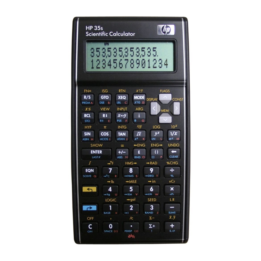
HP 35s User Manual
Scientific calculator
Hide thumbs
Also See for 35s:
- Quick start manual (60 pages) ,
- Instruction manual (9 pages) ,
- User manual (6 pages)

Related Manuals for HP 35s


Summary of Contents for HP 35s
- Page 1 HP 35s scientific calculator user's guide Edition 1 HP part number F2215AA-90001...
- Page 2 Notice REGISTER YOUR PRODUCT AT: www.register.hp.com THIS MANUAL AND ANY EXAMPLES CONTAINED HEREIN ARE PROVIDED “AS IS” AND ARE SUBJECT TO CHANGE WITHOUT NOTICE. HEWLETT-PACKARD COMPANY MAKES NO WARRANTY OF ANY KIND WITH REGARD TO THIS MANUAL, INCLUDING, BUT NOT LIMITED TO, THE IMPLIED WARRANTIES OF MERCHANTABILITY, NON- INFRINGEMENT AND FITNESS FOR A PARTICULAR PURPOSE.
-
Page 3: Table Of Contents
Contents Part 1. Basic Operation 1. Getting Started...1-1 Important Preliminaries ... 1-1 Turning the Calculator On and Off ... 1-1 Adjusting Display Contrast... 1-1 Highlights of the Keyboard and Display ... 1-2 Shifted Keys ... 1-2 Alpha Keys ... 1-3 Cursor Keys ... - Page 4 Complex number display format (, , ·‚)...1-24 SHOWing Full 12–Digit Precision ...1-25 Fractions ...1-26 Entering Fractions...1-26 Messages...1-27 Calculator Memory ...1-28 Checking Available Memory ...1-28 Clearing All of Memory ...1-29 2. RPN: The Automatic Memory Stack ...2-1 What the Stack Is...2-1 The X and Y–Registers are in the Display...2-3...
- Page 5 Using the MEM Catalog ... 3-4 The VAR catalog... 3-4 Arithmetic with Stored Variables... 3-6 Storage Arithmetic ... 3-6 Recall Arithmetic... 3-7 Exchanging x with Any Variable ... 3-8 The Variables "I" and "J"... 3-9 4. Real–Number Functions ...4-1 Exponential and Logarithmic Functions ... 4-1 Quotient and Remainder of Division...
- Page 6 5. Fractions...5-1 Entering Fractions ...5-1 Fractions in the Display...5-2 Display Rules ...5-2 Accuracy Indicators...5-3 Changing the Fraction Display...5-4 Setting the Maximum Denominator ...5-4 Choosing a Fraction Format ...5-6 Examples of Fraction Displays...5-8 Rounding Fractions...5-8 Fractions in Equations...5-9 Fractions in Programs ...5-10 6.
- Page 7 Operator Precedence ... 6-14 Equation Functions... 6-16 Syntax Errors... 6-19 Verifying Equations... 6-19 7. Solving Equations...7-1 Solving an Equation... 7-1 Solving built-in Equation ... 7-6 Understanding and Controlling SOLVE... 7-7 Verifying the Result ... 7-7 Interrupting a SOLVE Calculation... 7-8 Choosing Initial Guesses for SOLVE ...
- Page 8 Dot product ...10-4 Angle between vectors...10-5 Vectors in Equations ...10-6 Vectors in Programs... 10-7 Creating Vectors from Variables or Registers ...10-8 11.Base Conversions and Arithmetic and Logic...11-1 Arithmetic in Bases 2, 8, and 16 ...11-4 The Representation of Numbers ...11-6 Negative Numbers...11-6 Range of Numbers ...11-7 Windows for Long Binary Numbers...11-8...
- Page 9 Part 2. Programming 13.Simple Programming...13-1 Designing a Program ... 13-3 Selecting a Mode ... 13-3 Program Boundaries (LBL and RTN) ... 13-4 Using RPN, ALG and Equations in Programs ... 13-4 Data Input and Output ... 13-5 Entering a Program... 13-6 Clear functions and backspace key...
- Page 10 Clearing One or More Programs...13-23 The Checksum ...13-23 Nonprogrammable Functions ...13-24 Programming with BASE ...13-24 Selecting a Base Mode in a Program...13-25 Numbers Entered in Program Lines ...13-25 Polynomial Expressions and Horner's Method...13-26 14.Programming Techniques ...14-1 Routines in Programs ...14-1 Calling Subroutines (XEQ, RTN) ...14-1 Nested Subroutines ...14-2 Branching (GTO) ...14-4...
- Page 11 A. Support, Batteries, and Service ... A-1 Calculator Support... A-1 Answers to Common Questions ... A-1 Environmental Limits... A-2 Changing the Batteries ... A-3 Testing Calculator Operation ... A-4 The Self–Test ... A-5 Warranty ... A-7 Service... A-8 Regulatory information ... A-12 Federal Communications Commission Notice ...
- Page 12 B. User Memory and the Stack...B-1 Managing Calculator Memory... B-1 Resetting the Calculator ... B-2 Clearing Memory... B-3 The Status of Stack Lift ... B-4 Disabling Operations... B-5 Neutral Operations ... B-5 The Status of the LAST X Register... B-6 Accessing Stack Register Contents ...
- Page 13 How SOLVE Finds a Root ... D-1 Interpreting Results... D-3 When SOLVE Cannot Find a Root ... D-8 Round–Off Error ... D-13 E. More about Integration... E-1 How the Integral Is Evaluated... E-1 Conditions That Could Cause Incorrect Results ... E-2 Conditions That Prolong Calculation Time...
- Page 14 Contents...
-
Page 15: Part 1. Basic Operation
Part 1 Basic Operation... -
Page 17: Getting Started
(which has OFF printed in yellow above it). Since the calculator has Continuous Memory, turning it off does not affect any information you've stored. To conserve energy, the calculator turns itself off after 10 minutes of inactivity. If you see the low–power indicator ( possible. -
Page 18: Highlights Of The Keyboard And Display
Press the appropriate shift key ( ) before pressing the key for the desired function. For example, to turn the calculator off, press and release the shift key, then press Getting Started... -
Page 19: Alpha Keys
Pressing turns on the corresponding the top of the display. The annunciator remains on until you press the next key. To cancel a shift key (and turn off its annunciator), press the same shift key again. Alpha Keys Left-shifted function Right-shifted... -
Page 20: Backspacing And Clearing
Getting Started Keys for Clearing Description behaves similarly when the calculator is in erases the character immediately to the left of the insert deletes the entire equation. erases the character to the left of the insert ... - Page 21 Keys for Clearing (continued) Description The CLEAR menu ( ) contains options for clearing x (the number in the X-register), all direct variables, all of memory, all statistical data, all stacks and indirect variables. ...
-
Page 22: Using Menus
Using Menus There is a lot more power to the HP 35s than what you see on the keyboard. This is because 16 of the keys are menu keys. There are 16 menus in all, which provide many more functions, or more options for more functions. - Page 23 FLAGS Functions to set, clear, and test flags. Comparison tests of the X–and Y–registers. Comparison tests of the X–register and zero. Memory status (bytes of memory available); catalog of variables; catalog of programs (program labels). MODE ...
-
Page 24: Exiting Menus
8 Menus help you execute dozens of functions by guiding you to them. You don’t have to remember the names of all the functions built into the calculator nor search through the functions printed on the keyboard. Exiting Menus Whenever you execute a menu function, the menu automatically disappears, as in the above example. -
Page 25: Rpn And Alg Modes
RPN and ALG Modes The calculator can be set to perform arithmetic operations in either RPN (Reverse Polish Notation) or ALG (Algebraic) mode. In Reverse Polish Notation (RPN) mode, the intermediate results of calculations are stored automatically; hence, you do not have to use parentheses. - Page 26 To select ALG mode: 9{ Press () to set the calculator to ALG mode. When the calculator is in ALG mode, the ALG annunciator is on. Example: Suppose you want to calculate 1 + 2 = 3. In RPN mode, you enter the first number, press the...
-
Page 27: Undo Key
Undo key The Undo Key The operation of the Undo key depends on the calculator context, but serves largely to recover from the deletion of an entry rather than to undo any arbitrary operation. See The Last X Register in Chapter 2 for details on recalling the entry in line 2 of the display after a numeric function is executed. -
Page 28: The Display And Annunciators
The Display and Annunciators The display comprises two lines and annunciators. Entries with more than 14 characters will scroll to the left. During input, the entry is displayed in the first line in ALG mode and the second line in RPN mode. Every calculation is displayed in up to 14 digits, including an exponent value up to three digits. - Page 29 Annunciator PRGM 0 1 2 3 4 RAD or GRAD HEX OCT BIN HP 35s Annunciators Meaning The " (Busy)" annunciator appears while an operation, equation, or program is executing. When in Fraction–display mode (press ), only one of the " " or " " halves of the "...
- Page 30 HP 35s Annunciators (continued) Annunciator A..Z 1-14 Getting Started Meaning There are more characters to the left or right in the display of the entry in line 1 or line 2. Both of these annunciators may appear...
-
Page 31: Keying In Numbers
. If the result of a calculation is beyond this range, the error message “” appears momentarily along with the overflow message is then replaced with the value closest to the overflow boundary that the calculator can display. The smallest numbers the calculator can distinguish -499 from zero are 10 . - Page 32 For example, instead of entering one million as 1000000 you can simply enter illustrates the process as well as how the calculator displays the result. Example: Suppose you want to enter Planck’s constant: 6.6261 10 Keys: ...
-
Page 33: Understanding Entry Cursor
If entry is terminated (no cursor), number. Try it! Range of Numbers and OVERFLOW The smallest number available on the calculator is –9.99999999999 the largest number is 9.99999999999 If a calculation produces a result that exceeds the largest possible number, –... -
Page 34: Performing Arithmetic Calculations
Performing Arithmetic Calculations The HP 35s can operate in either RPN mode or in Algebraic mode (ALG). These modes affect how expressions are entered. The following sections illustrate the entry differences for single argument (or unary) and two argument (or binary) operations. -
Page 35: Two Argument Or Binary Operations
Example: , first in RPN mode and then in ALG mode. Calculate 3.4 Keys: 9 () 9 () In the example, the square operator is shown on the key as SQ(). There are several single argument operators that display differently in ALG mode than they appear on the keyboard (and differently than they appear in RPN mode as well). - Page 36 Example Calculate 2+3 and , first in RPN mode and then in ALG mode. Keys: 9 () x 9 () x Õ In ALG mode, the infix operators are argument operations use function notation of the form f(x,y), where x and y are the first and second operands in order.
-
Page 37: Controlling The Display Format
For 10 or 11 places, press For example, in the number , the "7", "0", "8", and "9" are the decimal digits you see when the calculator is set to FIX 4 display mode. Any number that is too large (10 decimal–place setting will automatically be displayed in scientific format. - Page 38 , the "2", "3", "4", and "6" are the decimal digits you see when the calculator is set to SCI 4 display mode. The "5" following the "E" is the exponent of 10: 1.2346 If you enter or calculate a number that has more than 12 digits, the additional precision is not maintained.
-
Page 39: Periods And Commas In Numbers () ()
Periods and Commas in Numbers () () The HP 35s uses both periods and commas to make numbers easier to read. You can select either the period or the comma as the decimal point (radix). In addition, you can choose whether or not to separate digits into groups of three using thousand separators. -
Page 40: Complex Number Display Format (, , ·')
Example Enter the number 12,345,678.90 and change the decimal point to the comma. Then choose to have no thousand separator. Finally, return to the default settings. This example uses RPN mode. Keys: 8 ( ) 8 () 8... -
Page 41: Showing Full 12-Digit Precision
For example, in the number 14.8745632019, you see only "14.8746" when the display mode is set to FIX 4, but the last six digits ("632019") are present internally in the calculator. To temporarily display a number in full precision, press you the mantissa (but no exponent) of the number for as long as you hold down Î... -
Page 42: Fractions
The HP 35s allows you to enter and operate on fractions, displaying them as either decimals or fractions. The HP 35s displays fractions in the form a b/c, where a is an integer and both b and c are counting numbers. In addition, b is such that 0 b<c and c is such that 1<c 4095. -
Page 43: Messages
É Refer to chapter 5, "Fractions," for more information about using fractions. Messages The calculator responds to error conditions by displaying the Usually, a message will accompany the error annunciator as well. To clear a message, press stack as it was before the error. In ALG mode, you will return to the last expression with the edit cursor at the position of the error so that you can correct it. -
Page 44: Calculator Memory
All displayed messages are explained in appendix F, "Messages". Calculator Memory The HP 35s has 30KB of memory in which you can store any combination of data (variables, equations, or program lines). Checking Available Memory ... -
Page 45: Clearing All Of Memory
Clearing All of Memory Clearing all of memory erases all numbers, equations, and programs you've stored. It does not affect mode and format settings. (To clear settings as well as data, see "Clearing Memory" in appendix B.) To clear all of memory: ... - Page 46 1-30 Getting Started...
-
Page 47: Rpn: The Automatic Memory Stack
What the Stack Is Automatic storage of intermediate results is the reason that the HP 35s easily processes complex calculations, and does so without parentheses. The key to automatic storage is the automatic, RPN memory stack. - Page 48 The most "recent" number is in the X–register: this is the number you see in the second line of the display. Every register is separated into three parts: A real number or a 1-D vector will occupy part 1; part 2 and part 3 will be null in this case.
-
Page 49: The X And Y-Registers Are In The Display
The X and Y–Registers are in the Display The X and Y–Registers are what you see except when a menu, a message, an equation line ,or a program line is being displayed. You might have noticed that several function names include an x or y. This is no coincidence: these letters refer to the X–... -
Page 50: Exchanging The X- And Y-Registers In The Stack
What was in the X–register rotates into the T–register, the contents of the T–register rotate into the Z–register, etc. Notice that only the contents of the registers are rolled — the registers themselves maintain their positions, and only the X– and Y–register's contents are displayed. -
Page 51: Arithmetic - How The Stack Does It
Arithmetic – How the Stack Does It The contents of the stack move up and down automatically as new numbers enter the X–register (lifting the stack) and as operators combine two numbers in the X– and Y–registers to produce one new number in the X–register (dropping the stack). Suppose the stack is filled with the numbers 1, 2, 3, and 4. -
Page 52: How Enter Works
How ENTER Works You know that separates two numbers keyed in one after the other. In terms of the stack, how does it do this? Suppose the stack is again filled with 1, 2, 3, and 4. Now enter and add two new numbers: ... -
Page 53: How To Clear The Stack
Filling the stack with a constant The replicating effect of (from T into Z) allows you to fill the stack with a numeric constant for calculations. Example: Given bacterial culture with a constant growth rate of 50% per day, how large would a population of 100 be at the end of 3 days? ... -
Page 54: The Last X Register
1. Lifts the stack 2. Lifts the stack and replicates the X–register. 3. Overwrites the X–register. 4. Clears x by overwriting it with zero. 5. Overwrites x (replaces the zero.) The LAST X Register The LAST X register is a companion to the stack: it holds the number that was in the X–register before the last numeric function was executed. -
Page 55: Correcting Mistakes With Last X
Correcting Mistakes with LAST X Wrong Single Argument Function If you execute the wrong single argument function, use the number so you can execute the correct function. (Press clear the incorrect result from the stack.) Since from these functions in the same manner as from single argument functions. Example: Suppose that you had just computed ln 4.7839 its square root, but pressed... -
Page 56: Reusing Numbers With Last X
Example: Suppose you made a mistake while calculating There are three kinds of mistakes you could have made: Wrong Calculation: Reusing Numbers with LAST X You can use Remember to enter the constant second, just before executing the arithmetic operation, so that the constant is the last number in the X–register, and therefore can be saved and retrieved with Example:... - Page 57 Keys: Example: Two close stellar neighbors of Earth are Rigel Centaurus (4.3 light–years away) and Sirius (8.7 light–years away). Use c, the speed of light (9.5 to convert the distances from the Earth to these stars into meters: To Rigel Centaurus: 4.3 yr To Sirius: 8.7 yr (9.5...
-
Page 58: Chain Calculations In Rpn Mode
If you were working out this problem on paper, you would first calculate the intermediate result of (12 + 3) ... … then you would multiply the intermediate result by 7: Evaluate the expression in the same way on the HP 35s, starting inside the parentheses. Keys: ... - Page 59 + 6). Finally, you would multiply the two intermediate results to get the answer. Work through the problem the same way with the HP 35s, except that you don't have to write down intermediate answers—the calculator remembers them for you.
-
Page 60: Exercises
Exercises Calculate: 3805 Solution: Calculate: × Solution: Calculate: (10 – 5) [(17 – 12) Solution: Order of Calculation We recommend solving chain calculations by working from the innermost parentheses outward. However, you can also choose to work problems in a left– to–right order. - Page 61 by starting with the innermost parentheses (7 as you would with pencil and paper. The keystrokes were If you work the problem from left–to–right, press This method takes one additional keystroke. Notice that the first intermediate result is still the innermost parentheses (7 right is that you don't have to use ...
-
Page 62: More Exercises
More Exercises Practice using RPN by working through the following problems: Calculate: (14 + 12) (18 – 12) A Solution: Calculate: – (13 9) + 1/7 = 412.1429 A Solution: Calculate: × ÷ − Solution: ... - Page 63 A Solution: 2-17 RPN: The Automatic Memory Stack...
- Page 64 2-18 RPN: The Automatic Memory Stack...
-
Page 65: Storing Data Into Variables
Storing Data into Variables The HP 35s has 30 KB of memory, in which you can store numbers, equations, and programs. Numbers are stored in locations called variables, each named with a letter from A through Z. (You can choose the letter to remind you of what is stored there, such as B for bank balance and C for the speed of light.) -
Page 66: Storing And Recalling Numbers
Numbers and vectors are stored into, and recalled from, lettered variables by means of the Store ( real or complex, decimal or fraction, base 10 or other as supported by the HP 35s. To store a copy of a displayed number (X–register) to a direct variable: ... - Page 67 Example: In this example, we recall the value of 1.75 that we stored in the variable G in the last example. This example assumes the HP 35s is still in ALG mode at the start. Keys: G In ALG mode, Recall can be used to paste a variable into an expression in the command line.
-
Page 68: Viewing A Variable
Keys: 9 () Viewing a Variable The VIEW command ( that value to the x-register. The display takes the form Variable=Value. If the number has too many digits to fit into the display, use missing digits. To cancel the VIEW display, press is most often used in programming but it is useful anytime you want to view a variable’s value without affecting the stack. - Page 69 Example: In this example, we store 3 in C, 4 in D, and 5 in E. Then we view these variables via the VAR Catalog and clear them as well. This example uses RPN mode. Keys: ( ) C D E...
-
Page 70: Arithmetic With Stored Variables
To leave the VAR catalog at any time, press either . An alternate method to clearing a variable is simply to store the value zero in it. Finally, you can clear all direct variables by pressing (). -
Page 71: Recall Arithmetic
Recall Arithmetic Recall arithmetic uses in the X–register using a recalled number and to leave the result in the display. Only the X–register is affected. The value in the variable remains the same and the result replaces the value in the x-register. New x = Previous x {+, –, , } Variable For example, suppose you want to divide the number in the X–register (3, displayed) by the value in A(12). -
Page 72: Exchanging X With Any Variable
Example: Suppose the variables D, E, and F contain the values 1, 2, and 3. Use storage arithmetic to add 1 to each of those variables. Keys: D E F D E F D ... -
Page 73: The Variables "I" And "J
Example: Keys: A _ A A The Variables "I" and "J" There are two variables that you can access directly: the variables I and J. Although they store values as other variables do, I and J are special in that they can be used to refer to other variables, including the statistical registers, using the (I) and (J) commands. - Page 74 3-10 Storing Data into Variables...
-
Page 75: Real-Number Functions
(root–finding, integrating, complex numbers, base conversions, and statistics) are described in later chapters. The examples in this chapter all assume the HP 35s is in RPN mode. Exponential and Logarithmic Functions Put the number in the display, then execute the function- there is no need to press ... -
Page 76: Quotient And Remainder Of Division
To Calculate: Natural logarithm (base e) Common logarithm (base 10) Natural exponential Common exponential (antilogarithm) Quotient and Remainder of Division You can use integer quotient and integer remainder, respectively, from the division of two integers. 1. Key in the first integer. ... -
Page 77: Trigonometry
12 digits of (The number displayed depends on the display format.) Because function that returns an approximation of Note that the calculator cannot exactly represent , since number. Press: . For y 0, x must be an integer. -
Page 78: Setting The Angular Mode
Arc cosine of x. Arc tangent of x. Calculations with the irrational number Note exactly by the 15–digit internal precision of the calculator. This is particularly noticeable in trigonometry. For example, the calculated sin small number close to zero. Real–Number Functions . - Page 79 Example: Show that cosine (5/7) radians and cosine 128.57° are equal (to four significant digits). Keys: 9 () 9 () Programming Note: Equations using inverse trigonometric functions to determine an angle , often look something like this: If x = 0, then y x is undefined, resulting in the error: ...
-
Page 80: Hyperbolic Functions
Hyperbolic Functions With x in the display: To Calculate: Hyperbolic sine of x (SINH). Hyperbolic cosine of x (COSH). Hyperbolic tangent of x (TANH). Hyperbolic arc sine of x (ASINH). Hyperbolic arc cosine of x (ACOSH). Hyperbolic arc tangent of x (ATANH). Percentage Functions The percentage functions are special (compared with preserve the value of the base number (in the Y–register) when they return the result... - Page 81 Keys: 8 () Suppose that the $15.76 item cost $16.12 last year. What is the percentage change from last year's price to this year's? Keys: 8 () The order of the two numbers is important for the %CHG function. Note The order affects whether the percentage change is considered positive or negative.
-
Page 82: Physics Constants
Physics Constants There are 41 physics constants in the CONST menu. You can press to view the following items. Items Description Speed of light in vacuum Standard acceleration of gravity Newtonian constant of gravitation Molar volume of ideal gas ... - Page 83 Items Description Muon magnetic moment Classical electron radius Characteristic impendence of vacuum Compton wavelength Neutron Compton wavelength Proton Compton wavelength Fine structure constant Stefan–Boltzmann constant Celsius temperature Standard atmosphere a Proton gyromagnetic ratio γ...
-
Page 84: Conversion Functions
Conversion Functions The HP 35s supports four types of conversions. You can convert between: rectangular and polar formats for complex numbers degrees, radians, and gradients for angle measures decimal and hexagesimal formats for time (and degree angles) various supported units (cm/in, kg/lb, etc) With the exception of the rectangular and polar conversions, each of the conversions is associated with a particular key. - Page 85 To convert between rectangular and polar coordinates: The format for representing complex numbers is a mode setting. You may enter a complex number in any format; upon entry, the complex number is converted to the format determined by the mode setting. Here are the steps required to set a complex number format: 8 1.
- Page 86 8 () 6 Example: Conversion with Vectors. Engineer P.C. Bord has determined that in the RC circuit shown, the total impedance is 77.8 ohms and voltage lags current by 36.5º. What are the values of resistance R and capacitive reactance X Use a vector diagram as shown, with impedance equal to the polar magnitude, r, and voltage lag equal to the angle, , in degrees.
-
Page 87: Time Conversions
Time Conversions The HP 35s can convert between decimal and hexagesimal formats for numbers. This is especially useful for time and angles measured in degrees. For example, in decimal format an angle measured in degrees is expressed as D.ddd…, while in hexagesimal the same angle is represented as D.MMSSss, where D is the integer... -
Page 88: Unit Conversions
To convert an angle between degrees and radians: Example In this example, we convert an angle measure of 30 to /6 radians. Keys: µ Unit Conversions The HP 35s has ten unit–conversion functions on the keyboard: ºF, gal, To Convert: 1 lb 1 kg 32 ºF ºC... -
Page 89: Probability Functions
Probability Functions Factorial To calculate the factorial of a displayed non-negative integer x (0 253), press * (the right–shifted key). Gamma To calculate the gamma function of a noninteger x, (x), key in (x – 1) and press ... - Page 90 You can store a new seed with the SEED function. If memory is cleared, the seed is reset to zero. A seed of zero will result in the calculator generating its own seed. Example: Combinations of People.
-
Page 91: Parts Of Numbers
Parts of Numbers These functions are primarily used in programming. Integer part To remove the fractional part of x and replace it with zeros, press (). (For example, the integer part of 14.2300 is 14.0000.) Fractional part To remove the integer part of x and replace it with zeros, press (). - Page 92 Greatest integer To obtain the greatest integer equal to or less than given number, press (). Example: This example summarizes many of the operations that extract parts of numbers. To calculate: The integer part of 2.47 The fractional part of 2.47 The absolute value of –7 The sign value of 9 The greatest integer equal to...
-
Page 93: Fractions
Fractions In Chapter 1, the section Fractions introduced the basics of entering, displaying, and calculating with fractions. This chapter gives more information on these topics. Here is a short review of entering and displaying fractions: To enter a fraction, press number and again between the numerator and denominator of the fractional part of the number. -
Page 94: Fractions In The Display
Display Rules The fraction you see may differ from the one you enter. In its default condition, the calculator displays a fractional number according to the following rules. (To change the rules, see "Changing the Fraction Display" later in this chapter.) The number has an integer part and, if necessary, a proper fraction (the numerator is less than the denominator). -
Page 95: Accuracy Indicators
Accuracy Indicators The accuracy of a displayed fraction is indicated by the the right of the display. The calculator compares the value of the fractional part of the internal 12–digit number with the value of the displayed fraction: If no indicator is lit, the fractional part of the internal 12–digit value exactly matches the value of the displayed fraction. -
Page 96: Changing The Fraction Display
Setting the Maximum Denominator For any fraction, the denominator is selected based on a value stored in the calculator. If you think of fractions as a b/c, then /c corresponds to the value that controls the denominator. The /c value defines only the maximum denominator used in Fraction–display mode —... - Page 97 To set the maximum denominator value, enter the value and then press . Fraction-display mode will be automatically enabled. The value you enter cannot exceed 4095. To recall the /c value to the X–register, press To restore the default value to 4095, press greater than 4095 as the maximum denominator.
-
Page 98: Choosing A Fraction Format
The error message “ ” will be displayed. Choosing a Fraction Format The calculator has three fraction formats. The displayed fractions are always the most accurate fractions within the rules for the selected format. Most precise fractions. Fractions have any denominator up to the /c value, and they're reduced as much as possible. - Page 99 To Get This Fraction Format: Most precise Factors of denominator Fixed denominator You can change flags 8 and 9 to set the fraction format using the steps listed here. (Because flags are especially useful in programs, their use is covered in detail in chapter 14.) ...
-
Page 100: Examples Of Fraction Displays
Examples of Fraction Displays The following table shows how the number 2.77 is displayed in the three fraction formats for two /c values. Fraction Format Most Precise Factors of Denominator Fixed Denominator The following table shows how different numbers are displayed in the three fraction formats for a /c value of 16. -
Page 101: Fractions In Equations
Example: Suppose you have a 56 sections. How wide is each section, assuming you can conveniently measure inch increments? What's the cumulative roundoff error? Keys: D D () Fractions in Equations You can use a fraction in an equation. -
Page 102: Fractions In Programs
Fractions in Programs You can use a fraction in a program just as you can in an equation; numerical values are shown in their entered form. When you're running a program, displayed values are shown using Fraction– display mode if it's active. If you're prompted for values by INPUT instructions, you may enter fractions. -
Page 103: Entering And Evaluating Equations
volume of 16 inches of 2 by storing the equation, you get the HP 35s to "remember" the relationship between diameter, length, and volume — so you can use it many times. Put the calculator in Equation mode and type in the equation using the following keystrokes: V = .25... - Page 104 Keys: or the current equation in line 2 _ _ _ D _ _ By comparing the checksum and length of your equation with those in the example, you can verify that you've entered the equation properly.
-
Page 105: Summary Of Equation Operations
Summary of Equation Operations All equations you create are saved in the equation list. This list is visible whenever you activate Equation mode. You use certain keys to perform operations involving equations. They're described in more detail later. When displaying equations in the equation list, two equations are displayed at a time. -
Page 106: Entering Equations Into The Equation List
Variables in Equations You can use any of the calculator's variables in an equation: A through Z,(I) and (J). You can use each variable as many times as you want.(For information about (I) and (J), see "Indirectly Addressing Variables and Labels" in chapter 14.) To enter a variable in an equation, press A..Z annunciator shows that you can press a variable key to enter its name in the... -
Page 107: Numbers In Equations
, and Functions in Equations You can enter many HP 35s functions in an equation. A complete list is given under “Equation Functions” later in this chapter. Appendix G, "Operation Index," also gives this information. When you enter an equation, you enter functions in about the same way you put... -
Page 108: Parentheses In Equations
Parentheses in Equations You can include parentheses in equations to control the order in which operations are performed. Press "Operator Precedence" later in this chapter.) Example: Entering an Equation. Enter the equation r = 2 Keys: _ ... - Page 109 To display equations: 1. Press . This activates Equation mode and turns on the EQN annunciator. The display shows an entry from the equation list: if the equation pointer is at the top of the list. The current equation (the last equation you viewed).
-
Page 110: Editing And Clearing Equations
Editing and Clearing Equations You can edit or clear an equation that you're typing. You can also edit or clear equations saved in the equation list. However, you cannot edit or clear the two built- in equations 2*2 lin. solve and 3*3 lin. solve. If you attempt to insert a equation between the two built-in equations, the new equation will be inserted after 3*3 lin. -
Page 111: Types Of Equations
Types of Equations The HP 35s works with three types of equations: Equalities. The equation contains an "=", and the left side contains more than just a single variable. For example, x Assignments. The equation contains an "=", and the left side contains just a single variable. -
Page 112: Evaluating Equations
For this calculation, "=" in an equation is essentially treated as "–". The value is a measure of how well the equation balances. The HP 35s has two keys for evaluating equations: actions differ only in how they evaluate assignment equations: ... -
Page 113: Using Enter For Evaluation
2. Press needed. (If the base of a number in the equation is different from the current base, the calculator automatically changes the result to the current base.) 3. For each prompt, enter the desired value: If the displayed value is good, press If you want a different value, type the value and press "Responding to Equation Prompts"... -
Page 114: Using Xeq For Evaluation
If the equation is an assignment, only the right–hand side is evaluated. The result is returned to the X–register and stored in the left–hand variable, then the variable is viewed in the display. Essentially, the left–hand variable. If the equation is an equality or expression, the entire equation is evaluated —... -
Page 115: Responding To Equation Prompts
Example: Evaluating an Equation with XEQ. Use the results from the previous example to find out how much the volume of the pipe changes if the diameter is changed to 35.5 millimeters. Keys: ... -
Page 116: The Syntax Of Equations
To change the number, type the new number and press number writes over the old value in the X–register. You can enter a number as a fraction if you want. If you need to calculate a number, use normal keyboard calculations, then press ... - Page 117 Order Parentheses Functions Power ( Unary Minus ( Multiply and Divide Add and Subtract Equality So, for example, all operations inside parentheses are performed before operations outside the parentheses. Examples: Equations Operation a + (b/c) = 12 (a + b) / c = 12 [%CHG ((t + 12), (a –...
-
Page 118: Equation Functions
Equation Functions The following table lists the functions that are valid in equations. Appendix G, "Operation Index" also gives this information. INTG SINH COSH SEED – x ˆ For convenience, prefix–type functions, which require one or two arguments, display a left parenthesis when you enter them. The prefix functions that require two arguments are %CHG, XROOT, IDIV, RMDR, nCr and nPr. - Page 119 The following equation calculates the perimeter of a trapezoid. This is how the equation might appear in a book: Perimeter = a + b + h ( The following equation obeys the syntax rules for HP 35s equations: Entering and Evaluating Equations Equation function...
- Page 120 Single letter name The next equation also obeys the syntax rules. This equation uses the inverse function, , instead of the fractional form, . Notice that the SIN function is "nested" inside the INV function. (INV is typed by Example: Area of a Polygon.
-
Page 121: Syntax Errors
You have to edit the equation to correct the error. (See "Editing and Clearing Equations" earlier in this chapter.) By not checking equation syntax until evaluation, the HP 35s lets you create "equations" that might actually be messages. This is especially useful in programs, as described in chapter 13. - Page 122 Keys: × as required) (hold) (release) 6-20 Entering and Evaluating Equations Display: Description: Displays the desired equation. Display equation's checksum and length. Redisplays the equation. Leaves Equation mode.
-
Page 123: Solving Equations
Solving Equations In chapter 6 you saw how you can use to find the value of the left–hand variable in an assignment–type equation. Well, you can use SOLVE to find the value of any variable in any type of equation. For example, consider the equation –... - Page 124 D-value(which should be zero). For some complicated mathematical conditions, a definitive solution cannot be found — and the calculator displays . See "Verifying the Result" later in this chapter, and "Interpreting Results" and "When SOLVE Cannot Find a Root"...
- Page 125 Keys: () Ö () G g (acceleration due to gravity) is included as a variable so you can change it for different units (9.8 m/s Calculate how many meters an object falls in 5 seconds, starting from rest. Since Equation mode is turned on and the desired equation is already in the display, you can start solving for D: Keys:...
- Page 126 Keys: Example: Solving the Ideal Gas Law Equation. The Ideal Gas Law describes the relationship between pressure, volume, temperature, and the amount (moles) of an ideal gas: where P is pressure (in atmospheres or N/m number of moles of gas, R is the universal gas constant (0.0821 liter–atm/mole–K or 8.314 J/mole–K), and T is temperature (Kelvins: K=°C + 273.1).
- Page 127 A 2–liter bottle contains 0.005 moles of carbon dioxide gas at 24°C. Assuming that the gas behaves as an ideal gas, calculate its pressure. Since Equation mode is turned on and the desired equation is already in the display, you can start solving for P: Keys: P...
-
Page 128: Solving Built-In Equation
2*2 linear equation system or x, y and z for a 3*3 linear equation system. The result will be saved in variables x, y, and z. The calculator can detect cases with infinitely many solutions or no solutions. Example: solve the x,y in simultaneous equations Keys: ... -
Page 129: Understanding And Controlling Solve
Some equations are more difficult to solve than others. In some cases, you need to enter initial guesses in order to find a solution. (See "Choosing Initial Guesses for SOLVE," below.) If SOLVE is unable to find a solution, the calculator displays . -
Page 130: Interrupting A Solve Calculation
If a calculation ends with the , the calculator could not converge on a root. (You can see the value in the X–register — the final estimate of the root — by ... - Page 131 (If such is the case, the calculator changes one guess slightly so that it has two different guesses.) Entering your own guesses has the following advantages: By narrowing the range of search, guesses can reduce the time to find a solution.
- Page 132 Example: Using Guesses to Find a Root. Using a rectangular piece of sheet metal 40 cm by 80 cm, form an open–top box having a volume of 7500 cm amount to be folded up along each of the four sides) that gives the specified volume.
- Page 133 4 H Õ H It seems reasonable that either a tall, narrow box or a short, flat box could be formed having the desired volume. Because the taller box is preferred, larger initial estimates of the height are reasonable. However, heights greater than 20 cm are not physically possible because the metal sheet is only 40 cm wide.
-
Page 134: For More Information
The dimensions of the desired box are 50 15 cm. If you ignored the upper limit on the height (20 cm) and used initial estimates of 30 and 40 cm, you would obtain a height of 42.0256 cm — a root that is physically meaningless. If you used small initial estimates such as 0 and 10 cm, you would obtain a height of 2.9774 cm —... -
Page 135: Integrating Equations
Integrating Equations Many problems in mathematics, science, and engineering require calculating the definite integral of a function. If the function is denoted by f(x) and the interval of integration is a to b, then the integral can be expressed mathematically as The quantity I can be interpreted geometrically as the area of a region bounded by the graph of the function f(x), the x–axis, and the limits x = a and x = b (provided that f(x) is nonnegative throughout the interval of integration). -
Page 136: Integrating Equations ( ∫ Fn)
4. Select the variable of integration: Press calculation. uses far more memory than any other operation in the calculator. If executing causes a message, refer to appendix B. You can halt a running integration calculation by pressing message “”... - Page 137 Example: Bessel Function. The Bessel function of the first kind of order 0 can be expressed as Find the Bessel function for x–values of 2 and 3. Enter the expression that defines the integrand's function: Keys: Ö () () ...
- Page 138 Now calculate J (3) with the same limits of integration. You must re-specify the limits of integration (0, ) since they were pushed off the stack by the subsequent division by . Keys: ...
- Page 139 Enter the expression that defines the integrand's function: If the calculator attempted to evaluate this function at x = 0, the lower limit of integration, an error ( ) would result. However, the integration algorithm normally does not evaluate functions at either limit of integration, unless the endpoints of the interval of integration are extremely close together or the number of sample points is extremely large.
-
Page 140: Accuracy Of Integration
(and the greater the time required to calculate it). The fewer the number of digits displayed, the faster the calculation, but the calculator will presume that the function is accurate to the only number of digits specified. - Page 141 Example: Specifying Accuracy. With the display format set to SCI 2, calculate the integral in the expression for Si(2) (from the previous example). Keys: 8 () The integral is 1.61±0.0161. Since the uncertainty would not affect the approximation until its third decimal place, you can consider all the displayed digits in this approximation to be accurate.
-
Page 142: For More Information
For More Information This chapter gives you instructions for using integration in the HP 35s over a wide range of applications. Appendix E contains more detailed information about how the algorithm for integration works, conditions that could cause incorrect results and conditions that prolong calculation time, and obtaining the current approximation to an integral. -
Page 143: Operations With Complex Numbers
Operations with Complex Numbers The HP 35s can use complex numbers in the form It has operations for complex arithmetic (+, –, , ), complex trigonometry (sin, cos, tan), and the mathematics functions –z, 1/z, are complex numbers). The form, x+yi, is only available in ALG mode. -
Page 144: The Complex Stack
The Complex Stack A complex number occupies part 1 and part 2 of a stack level. In RPN mode, the complex number occupying part 1 and part 2 of the X-register is displayed in line 2, while the complex number occupying part 1 and part 2 of the Y-register is displayed in line 1. - Page 145 Functions for One Complex Number, z To Calculate: Change sign, –z Inverse, 1/z Natural log, ln z Natural antilog, e Sin z Cos z Tan z Absolute value, ABS(z) Argument value, ARG(z) To do an arithmetic operation with two complex numbers: 1.
- Page 146 Examples: Here are some examples of trigonometry and arithmetic with complex numbers: Evaluate sin (2i3) Keys: 8 ( ) 6 Evaluate the expression where z = 23 i 13, z Perform the calculation as Keys: 8 ( ) 6 6 6...
-
Page 147: Using Complex Numbers In Polar Notation
6 Evaluate , where z = (1i 1). Keys: 6 Using Complex Numbers in Polar Notation Many applications use real numbers in polar form or polar notation. These forms use pairs of numbers, as do complex numbers, so you can do arithmetic with these numbers by using the complex operations. - Page 148 170 lb 100 lb Keys: 9 () 8 ( ? ? ? Õ You can do a complex operation with numbers whose complex forms are different; however, the result form is dependent on the setting in Operations with Complex Numbers Display: ...
-
Page 149: Complex Numbers In Equations
Evaluate 1i1+3 10+5 30 Keys: 9 () 8 ( 6 ? ? Complex Numbers in Equations You can type complex numbers in equations. When an equation is displayed, all numeric forms are shown as they were entered, like xiy, or r a When you evaluate an equation and are prompted for variable values, you may enter complex numbers. -
Page 150: Complex Number In Program
Complex Number in Program In a program, you can type a complex number. For example, 1i2+3 10+5 30 in program is: Program lines: (ALG mode) When you are running a program and are prompted for values by INPUT instructions, you can enter complex numbers. -
Page 151: Vector Arithmetic
Press and enter a third number for a 3-D vector. The HP 35s cannot handle vectors with more than 3 dimensions. Vector operations Addition and subtraction: The addition and subtraction of vectors require that two vector operands have the same length. - Page 152 Calculate [1.5,-2.2]+[-1.5,2.2] Keys: 9 () 3 3 Calculate [-3.4,4.5]-[2.3,1.4] Keys: 9 () 3 Õ 3 Multiplication and divisions by a scalar: Enter a vector Enter a scalar Press for multiplication or 10-2 Vector Arithmetic Display:...
-
Page 153: Absolute Value Of The Vector
Calculate [3,4]x5 Keys: 9 () 3 Calculate [-2,4]÷2 Keys: 9 () 3 Õ Absolute value of the vector The absolute value function “ABS”, when applied to a vector, produces the magnitude of the vector. For a vector A=(A1, A2, …An), the magnitude is defined ... -
Page 154: Dot Product
Dot product Function DOT is used to calculate the dot product of two vectors with the same length. Attempting to calculate the dot product of two vectors of different length causes an error message “ ”. For 2-D vectors: [A, B], [C, D], dot product is defined as [A, B] [C, D]= A x C +B x For 3-D vectors: [A, B, X], [C, D,Y], dot product is defined as [A, B, X] [C, D, Y]= A x C +B x D+X x Y Enter the first Vector... -
Page 155: Angle Between Vectors
Angle between vectors The angle between two vectors, A and B, can be found as ACOS(A B/ Find the angle between two vectors: A=[1,0],B=[0,1] Keys: 9 () 9 () 3 Õ 3 Õ 3 Õ 3 ... -
Page 156: Vectors In Equations
3 Vectors in Equations Vectors can be used in equations and in equation variables exactly like real numbers. A vector can be entered when prompted for a variable. Equations containing vectors can be solved, however the solver has limited ability if the unknown is a vector. -
Page 157: Vectors In Programs
Vectors in Programs Vectors can be used in program in the same way as real and complex numbers For example, [5, 6] +2 x [7, 8] x [9, 10] in a program is: Program lines: ... -
Page 158: Creating Vectors From Variables Or Registers
Creating Vectors from Variables or Registers It is possible to create vectors containing the contents of memory variables, stack registers, or values from the indirect registers, in run or program modes. In ALG mode, begin entering the vector by pressing similarly to ALG mode, except that the 3 pressing... -
Page 159: Base Conversions And Arithmetic And Logic
) allows you to enter numbers and force the display of ) provides access to logic functions. BASE Menu Description Decimal mode. This is the normal calculator mode Hexadecimal mode. when this mode is active. Numbers are displayed in hexadecimal format. In RPN mode, the keys ... - Page 160 placed at the end of a number means that this number is an octal number. To enter an octal number, type the number followed by “” placed at the end of a number means that this number is a ...
- Page 161 In RPN mode: When you enter a number in line 2, press mode, the calculator will convert the base of the numbers in line 1 and line 2, and the sign b/o/h will be added following the number to represent base 2/8/16.
-
Page 162: Arithmetic In Bases 2, 8, And 16
Menu label Logical bit-by-bit "AND" of two arguments. For example: AND(1100b,1010b)=1000b Logical bit-by-bit "XOR" of two arguments. For example: XOR(1101b,1011b)=110b Logical bit-by-bit "OR" of two arguments. For example: OR(1100b,1010b)=1110b Returns the one's complement of the argument. Each bit in ... - Page 163 The result of an operation is always an integer (any fractional portion is truncated). Whereas conversions change only the display of the number but not the actual number in the X–register, arithmetic does alter the number in the X–register. If the result of an operation cannot be represented in valid bits, the display shows ...
-
Page 164: The Representation Of Numbers
() () () () The Representation of Numbers Although the display of a number is converted when the base is changed, its stored form is not modified, so decimal numbers are not truncated — until they are used in arithmetic calculations. -
Page 165: Range Of Numbers
() Õ Õ () Range of Numbers The 36-bit binary number size determines the range of numbers that can be represented in hexadecimal (9 digits), octal (12 digits), and binary bases (36 digits), and the range of decimal numbers (11 digits) that can be converted to these other bases. -
Page 166: Windows For Long Binary Numbers
Equations and program are affected by the base setting and binary, octal and hexadecimal numbers can be entered in equation and in program as well as when the calculator prompts for a variable. Results will be displayed according to the current base. -
Page 167: Statistical Operations
Statistical Operations The statistics menus in the HP 35s provide functions to statistically analyze a set of one– or two–variable data(real numbers): Mean, sample and population standard deviations. Linear regression and linear estimation ( Weighted mean (x weighted by y). -
Page 168: Entering One-Variable Data
Y–register is accumulated as the y–value. For this reason, the calculator will perform linear regression and show you values based on y even when you have entered only x–data — or even if you have entered an unequal number of x–and y–values. - Page 169 them, then press register, and its x–value was saved in the LAST X register.) After deleting the incorrect statistical data, calculator will display the value of Y-register in line 1 and value of n in line 2. Example: Key in the x, y–values on the left, then make the corrections shown on the right:...
-
Page 170: Statistical Calculations
Statistical Calculations Once you have entered your data, you can use the functions in the statistics menus. Menu L.R. SUMS Mean Mean is the arithmetic average of a group of numbers. ... - Page 171 Example: Mean (One Variable). Production supervisor May Kitt wants to determine the average time that a certain process takes. She randomly picks six people, observes each one as he or she carries out the process, and records the time required (in minutes): 15.5 12.5 Calculate the mean of the times.
-
Page 172: Sample Standard Deviation
ÕÕ Sample Standard Deviation Sample standard deviation is a measure of how dispersed the data values are about the mean sample standard deviation assumes the data is a sampling of a larger, complete set of data, and is calculated using n – 1 as a divisor. ... -
Page 173: Population Standard Deviation
Population Standard Deviation Population standard deviation is a measure of how dispersed the data values are about the mean. Population standard deviation assumes the data constitutes the complete set of data, and is calculated using n as a divisor. ÕÕ Press values. - Page 174 Menu Key ˆ ˆ To find an estimated value for x (or y), key in a given hypothetical value for y (or x), then press To find the values that define the line that best fits your data, press followed by , , or .
- Page 175 ÕÕ () Õ Õ 8.50 7.50 6.50 5.50 b = 4.8560 4.50 ˆ ˆ ˆ ˆ ...
-
Page 176: Limitations On Precision Of Data
ˆ Õ Limitations on Precision of Data Since the calculator uses finite precision, it follows that there are limitations to calculations due to rounding. Here are two examples: Normalizing Close, Large Numbers The calculator might be unable to correctly calculate the standard deviation and linear regression for a variable whose data values differ by a relatively small amount. -
Page 177: Summation Values And The Statistics Registers
— values that are of interest when performing other statistical calculations in addition to those provided by the calculator. If you've entered statistical data, you can see the contents of the statistics registers. -
Page 178: Access To The Statistics Registers
× × Access to the Statistics Registers The statistics register assignments in the HP 35s are shown in the following table. Summation registers should be referred to by names and not by numbers in expression, equations and programs. Register... - Page 179 You can load a statistics register with a summation by storing the number (-27 through -32) of the register you want in I or J and then storing the summation (value 7 7 ). Similarly, you can press 7 ) to view (or recall)a register value —...
- Page 180 12-14 Statistical Operations...
-
Page 181: Part 2. Programming
Part 2 Programming... -
Page 183: Simple Programming
Simple Programming Part 1 of this manual introduced you to functions and operations that you can use manually, that is, by pressing a key for each individual operation. And you saw how you can use equations to repeat calculations without doing all of the keystrokes each time. - Page 184 RPN mode ALG mode This very simple program assumes that the value for the radius is in the X– register (the display) when the program starts to run. It computes the area and leaves it in the X–register.
-
Page 185: Designing A Program
XÕ Try running this program to find the area of a circle with a radius of 5: Keys: (In ALG mode) X We will continue using the above program for the area of a circle to illustrate programming concepts and methods. -
Page 186: Program Boundaries (Lbl And Rtn)
Program Boundaries (LBL and RTN) If you want more than one program stored in program memory, then a program needs a label to mark its beginning (such as ) and a return to mark its end (such as ). Notice that the line numbers acquire an ... -
Page 187: Data Input And Output
Using RPN operations (which work with the stack, as explained in chapter 2). Using ALG operations (as explained in appendix C). Using equations (as explained in chapter 6). The previous example used a series of RPN operations to calculate the area of the circle. -
Page 188: Entering A Program
Ø to find the label, and press 4. To record calculator operations as program instructions, press the same keys you would to do an operation manually. Remember that many functions don't appear on the keyboard but must be accessed using menus. -
Page 189: Clear Functions And Backspace Key
5. End the program with a return instruction, which sets the program pointer back to after the program runs. Press 6. Press Numbers in program lines are stored precisely as you entered them, and they're displayed using ALL or SCI format. (If a long number is shortened in the display, ... -
Page 190: Function Names In Programs
Now, erase line A002, and line A004 changes to “A003 GTO A002” Function Names in Programs The name of a function that is used in a program line is not necessarily the same as the function's name on its key, in its menu, or in an equation. - Page 191 A different checksum means the program was not entered exactly as given here. Example: Entering a Program with an Equation. The following program calculates the area of a circle using an equation, rather than using RPN operations like the previous program. Keys: (In RPN mode) ...
-
Page 192: Running A Program
Running a Program To run or execute a program, program entry cannot be active (no program–line numbers displayed; PRGM off). Pressing Executing a Program (XEQ) Press label to execute the program labeled with that letter: To execute a program from it’s beginning press A ... -
Page 193: Testing A Program
Testing a Program If you know there is an error in a program, but are not sure where the error is, then a good way to test the program is by stepwise execution. It is also a good idea to test a long or complicated program before relying on it. -
Page 194: Entering And Displaying Data
Entering and Displaying Data The calculator's variables are used to store data input, intermediate results, and final results. (Variables, as explained in chapter 3, are identified by a letter from A through Z, but the variable names have nothing to do with program labels.) In a program, you can get data in these ways: From an INPUT instruction, which prompts for the value of a variable. -
Page 195: Using Input For Entering Data
Using INPUT for Entering Data The INPUT instruction ( displays a prompt for the given variable. This display includes the existing value for the variable, such as where "R" is the variable's name, "?" is the prompt for information, and 0.0000 is the current value stored in the variable. - Page 196 2. In the beginning of the program, insert an INPUT instruction for each variable whose value you will need. Later in the program, when you write the part of the calculation that needs a given value, insert a that value back into the stack. Since the INPUT instruction also leaves the value you just entered in the Xñregister, you don't have to recall the variable at a later time ó...
-
Page 197: Using View For Displaying Data
To cancel the INPUT prompt, press remains in the X–register. If you press canceled INPUT prompt is repeated. If you press clears the number to zero. Press Using VIEW for Displaying Data The programmed VIEW instruction ( and displays and identifies the contents of the given variable, such as ... -
Page 198: Using Equations To Display Messages
Using Equations to Display Messages Equations aren't checked for valid syntax until they're evaluated. This means you can enter almost any sequence of characters into a program as an equation — you enter it just as you enter any equation. On any program line, press the equation. - Page 199 Keys: (In RPN mode) R H V R 4 R H S () V O L A R E A ...
-
Page 200: Displaying Information Without Stopping
Now find the volume and surface area–of a cylinder with a radius of 2 a height of 8 cm. Keys: (In RPN mode) C value value Displaying Information without Stopping Normally, a program stops when it displays a variable with VIEW or displays an equation message. -
Page 201: Stopping Or Interrupting A Program
Stopping or Interrupting a Program Programming a Stop or Pause (STOP, PSE) Pressing (run/stop) during program entry inserts a STOP instruction. This will display the contents of the X-register and halt a running program until you resume it by pressing RTN in order to end a program without returning the program pointer to the top of memory. -
Page 202: Editing A Program
Editing a Program You can modify a program in program memory by inserting, deleting, and editing program lines. If a program line contains an equation, you can edit the equation. To delete a program line: 1. Select the relevant program or routine and press program line that must be changed. -
Page 203: Program Memory
Viewing Program Memory Pressing toggles the calculator into and out of program entry (PRGM annunciator on, program lines displayed). When Program–entry mode is active, the contents of program memory are displayed. Program memory starts at . The list of program lines is circular, so you can wrap the program pointer from the bottom to the top and reverse. -
Page 204: Memory Usage
You can make more room available by clearing programs or other data. See "Clearing One or More Programs" below, or "Managing Calculator Memory" in appendix B. The Catalog of Programs (MEM) The catalog of programs is a list of all program labels with the number of bytes of memory used by each label and the lines associated with it. -
Page 205: Clearing One Or More Programs
If the known checksum and the one shown by your calculator are the same, then you have correctly entered all the lines of the program. To see your checksum: ... -
Page 206: Nonprogrammable Functions
In addition, each equation in a program has a checksum. See "To enter an equation in a program line" earlier in this chapter. Nonprogrammable Functions The following functions of the HP 35s are not programmable: () ... -
Page 207: Selecting A Base Mode In A Program
When writing programs that use numbers in a base other than 10, set the base mode both as the current setting for the calculator and in the program (as an instruction). -
Page 208: Polynomial Expressions And Horner's Method
Polynomial Expressions and Horner's Method Some expressions, such as polynomials, use the same variable several times for their solution. For example, the expression + Bx + Cx + Dx + E uses the variable x four different times. A program to calculate such an expression using RPN operations could repeatedly recall a stored copy of x from a variable. - Page 209 Keys: (In RPN mode) A X X X () Now evaluate this polynomial for x = 7. Keys: (In RPN mode) A...
- Page 210 A more general form of this program for any equation + Bx + Cx + Dx + E would be: ...
-
Page 211: Programming Techniques
Programming Techniques Chapter 13 covered the basics of programming. This chapter explores more sophisticated but useful techniques: Using subroutines to simplify programs by separating and labeling portions of the program that are dedicated to particular tasks. The use of subroutines also shortens a program that must perform a series of steps more than once. -
Page 212: Nested Subroutines
If you plan to have only one program in the calculator memory, you can separate the routine in various labels. If you plan to have more than one program in the calculator memory, it is better to have routines part of the main program label, starting at a specific line number. - Page 213 MAIN program (Top level) End of program Attempting to execute a subroutine nested more than 20 levels deep causes an error. Example: A Nested Subroutine. The following subroutine, labeled S, calculates the value of the expression as part of a larger calculation in a larger program. The subroutine calls upon another subroutine (a nested subroutine), labeled Q, to do the repetitive squaring and addition.
-
Page 214: Branching (Gto)
In RPN mode, ... -
Page 215: A Programmed Gto Instruction
A Programmed GTO Instruction The GTO label instruction (press a running program to the specified program line. The program continues running from the new location, and never automatically returns to its point of origination, so GTO is not used for subroutines. For example, consider the "Curve Fitting"... -
Page 216: Conditional Instructions
To : To a specific line number: A For example, . The display will show ” ” . If you want to go to the first line of a label, for example. A001: Conditional Instructions Another way to alter the sequence of program execution is by a conditional test, a true/false test that compares two numbers and skips the next program instruction if the proposition is false. -
Page 217: Tests Of Comparison (X?Y, X?0)
Select the category of comparison, then press the menu key for the conditional instruction you want. If you execute a conditional test from the keyboard, the calculator will display or . For example, if x =2 and y =7, test x y . - Page 218 ÕÕ In RPN mode ÕÕ In ALG mode Example: The "Normal and Inverse–Normal Distributions" program in chapter 16 uses the x y? conditional in routine T: Program Lines: (In RPN mode) ...
-
Page 219: Flags
Meanings of Flags The HP 35s has 12 flags, numbered 0 through 11. All flags can be set, cleared, and tested from the keyboard or by a program instruction. The default state of all 12 flags is clear. - Page 220 Flag Status Clear Fraction display off; display real (Default) numbers in the current display format. Fraction display on; display real numbers as fractions. 14-10 Programming Techniques Fraction–Control Flags Fraction denominators not greater than the /c value. Fraction denominators are factors of the /c Value.
- Page 221 Flag 10 controls program execution of equations: When flag 10 is clear (the default state), equations in running programs are evaluated and the result put on the stack. When flag 10 is set, equations in running programs are displayed as messages, causing them to behave like a VIEW statement: 1.
- Page 222 If it is not, then the next line is skipped. This is the "Do if True" rule, illustrated under "Conditional Instructions" earlier in this chapter. If you test a flag from the keyboard, the calculator will display "" or "". 14-12 Programming Techniques ...
- Page 223 It is good practice in a program to make sure that any conditions you will be testing start out in a known state. Current flag settings depend on how they have been left by earlier programs that have been run. You should not assume that any given flag is clear, for instance, and that it will be set only if something in the program sets it.
- Page 224 Example: Controlling the Fraction Display. The following program lets you exercise the calculator's fraction–display capability. The program prompts for and uses your inputs for a fractional number and a denominator (the /c value). The program also contains examples of how the three fraction–display flags (7, 8, and 9) and the "message–display"...
- Page 225 Program Lines: (In RPN mode) ...
-
Page 226: Loops
Use the above program to see the different forms of fraction display: Keys: (In RPN mode) F () Loops Branching backwards — that is, to a label in a previous line — makes it possible to execute part of a program more than once. -
Page 227: Conditional Loops (Gto)
This routine is an example of an infinite loop. It can be used to collect the initial data. After entering the three values, it is up to you to manually interrupt this loop by pressing label line number to execute other routines. Conditional Loops (GTO) When you want to perform an operation until a certain condition is met, but you don't know how many times the loop needs to repeat itself, you can create a loop... -
Page 228: Loops With Counters (Dse, Isg)
Loops with Counters (DSE, ISG) When you want to execute a loop a specific number of times, use the (increment; skip if greater than) or to) conditional function keys. Each time a loop function is executed in a program, it automatically decrements or increments a counter value stored in a variable. - Page 229 ii is the interval for incrementing and decrementing (must be two digits or unspecified). This value does not change. An unspecified value for ii is assumed to be 01 (increment/decrement by 1). Given the loop–control number ccccccc.fffii, DSE decrements ccccccc to ccccccc — ii, compares the new ccccccc with fff, and makes program execution skip the next program line if this ccccccc Given the loop–control number ccccccc.fffii, ISG increments ccccccc to ccccccc + ii,...
-
Page 230: Indirectly Addressing Variables And Labels
L Press number is now 11.0100. Indirectly Addressing Variables and Labels Indirect addressing is a technique used in advanced programming to specify a variable or label without specifying beforehand exactly which one. This is determined when the program runs, so it depends on the intermediate results (or input) of the program. -
Page 231: The Indirect Address, (I) And (J)
STO I RCL I STO +,–, RCL +,–, The Indirect Address, (I) and (J) Many functions that use A through Z (as variables or labels) can use (I) or (J) to refer to A through Z (variables or labels) or statistics registers indirectly. The function (I) or (J) uses the value in variable I to J to determine which variable, label, or register to address. - Page 232 If I/J contains: I<-32 or I>800 or variables undefined J<-32 or I>800 or variables undefined The INPUT(I) ,INPUT(J) and VIEW(I) ,VIEW(J)operations label the display with the name of the indirectly–addressed variable or register. The SUMS menu enables you to recall values from the statistics registers. However, you must use indirect addressing to do other operations, such as STO, VIEW, and INPUT.
-
Page 233: Program Control With (I)/(J)
STO(I)/(J) RCL(I)/(J) STO +, –, , , (I)/(J) RCL +, –, , , (I)/(J) X<>(I)/(J) FN=(I)/(J) You can not solve or integrate for unnamed variables or statistic registers. Program Control with (I)/(J) Since the contents of I can change each time a program runs — or even in different parts of the same program —... - Page 234 If you want to recall the value from an undefined storage address, the error message “ ”will be shown”. (See A014) The calculator allocates memory for variable 0 to the last non-zero variable. It is important to store 0 in variables after using them in order to release the memory.
-
Page 235: Solving And Integrating Programs
Solving and Integrating Programs Solving a Program In chapter 7 you saw how you can enter an equation — it's added to the equation list — and then solve it for any variable. You can also enter a program that calculates a function, and then solve it for any variable. - Page 236 2. Include an INPUT instruction for each variable, including the unknown. INPUT instructions enable you to solve for any variable in a multi–variable function. INPUT for the unknown is ignored by the calculator, so you need to write only one program that contains a separate INPUT instruction for every variable (including the unknown).
- Page 237 To begin, put the calculator in Program mode; if necessary, position the program pointer to the top of program memory. Keys: (In ALG mode) Type in the program: Program Lines: (In ALG mode) ...
- Page 238 Example: Program Using Equation. Write a program that uses an equation to solve the "Ideal Gas Law." Keys: (In RPN mode) (1) P V ...
- Page 239 Keys: (In RPN mode) L H P L Display: Stores previous pressure. Selects program “H.” Selects variable P; prompts for V. Retains 2 in V;...
-
Page 240: Using Solve In A Program
Using SOLVE in a Program You can use the SOLVE operation as part of a program. If appropriate, include or prompt for initial guesses (into the unknown variable and into the X–register) before executing the SOLVE variable instruction. The two instructions for solving an equation for an unknown variable appear in programs ... -
Page 241: Integrating A Program
Program Lines: (In RPN mode) Checksum and length: 62A0 11 Checksum and length: 221E 11 ... - Page 242 INPUT instructions enable you to integrate with respect to any variable in a multi–variable function. INPUT for the variable of integration is ignored by the calculator, so you need to write only one program that contains a separate INPUT instruction for every variable (including the variable of integration).
- Page 243 A function programmed as an equation is usually included as an expression specifying the integrand — though it can be any type of equation. If you want the equation to prompt for variable values instead of including INPUT instructions, make sure flag 11 is set. 4.
-
Page 244: Using Integration In A Program
Using Integration in a Program Integration can be executed from a program. Remember to include or prompt for the limits of integration before executing the integration, and remember that accuracy and execution time are controlled by the display format at the time the program runs. -
Page 245: Restrictions On Solving And Integrating
SOLVE instruction (produces an ∫ error). The SOLVE variable and ∫ FN d variable instructions in a program use one of the 20 pending subroutine returns in the calculator. (Refer to "Nested Subroutines" in chapter 14.) Solving and Integrating Programs... - Page 246 15-12 Solving and Integrating Programs...
-
Page 247: Statistics Programs
. (For definitions of these values, see "Linear Regression" in chapter 12.) Samples of the curves and the relevant equations are shown below. The internal regression functions of the HP 35s are used to compute the regression coefficients. 16-1 Statistics Programs... - Page 248 Straight Line Fit Logarithmic Curve Fit To fit logarithmic curves, values of x must be positive. To fit exponential curves, values of y must be positive. To fit power curves, both x and y must be positive. A error will occur if a negative number is entered for these cases. Data values of large magnitude but relatively small differences can incur problems of precision, as can data values of greatly different magnitudes.
- Page 249 Program Listing: Program Lines: (In RPN mode) This routine sets, the status for the straight–line model. Clears flag 0, the indicator for ln X. Clears flag 1, the indicator for In Y. ...
- Page 250 Program Lines: (In RPN mode) If flag 0 is set . . . . . . takes the natural log of the X–input. Stores that value for the correction routine. Prompts for and stores Y.
- Page 251 Program Lines: (In RPN mode) Displays, prompts for, and, if changed, stores x–value in X. If flag 0 is set . . . Branches to K001 Branches to M001 ...
- Page 252 Program Lines: (In RPN mode) Checksum and length: 889C 18 This subroutine calculates Calculates Returns to the calling routine. Checksum and length: 0DBE 18 ...
- Page 253 Program Lines: (In RPN mode) Calculates Goes to O005 Checksum and length: 8524 21 Determines if D001 or B001 should be run ...
- Page 254 Flags Used: Flag 0 is set if a natural log is required of the X input. Flag 1 is set if a natural log is required of the Y input. If flag 1 is set in routine N, then I001 is executed. If flag 1 is clear, G001 is executed.
- Page 255 13. For a new case, go to step 2. Variables Used: Statistics registers Example 1: Fit a straight line to the data below. Make an intentional error when keying in the third data pair and correct it with the undo routine. Also, estimate y for an x value of 37.
- Page 256 Now intentionally enter 379 instead of 37.9 so that you can see how to correct incorrect entries. Keys: (In RPN mode) U ...
-
Page 257: Normal And Inverse-Normal Distributions
Example 2: Repeat example 1 (using the same data) for logarithmic, exponential, and power curve fits. The table below gives you the starting execution label and the results (the correlation and regression coefficients and the x–... - Page 258 This program uses the built–in integration feature of the HP 35s to integrate the equation of the normal frequency curve. The inverse is obtained using Newton's method to iteratively search for a value of x which yields the given probability Q(x).
- Page 259 Program Listing: Program Lines: (In RPN mode) Checksum and length: 70BF 26 ...
- Page 260 Program Lines: (In RPN mode) Adds the correction to yield a new X Tests to see if the correction is significant. Goes back to start of loop if correction is significant. Continues if correction is not significant.
- Page 261 Program Lines: (In RPN mode) Checksum and length: B3EB 31 Flags Used: None. Remarks: The accuracy of this program is dependent on the display setting. For inputs in the area between ±3 standard deviations, a display of four or more significant figures is adequate for most applications.
- Page 262 4. After the prompt for S, key in the population standard deviation and press . (If the standard deviation is 1, just press 5. To calculate X given Q(X), skip to step 9 of these instructions. 6. To calculate Q(X) given X, 7.
- Page 263 D value Since your friend has been known to exaggerate from time to time, you decide to see how rare a "2 " date might be. Note that the program may be rerun simply by ...
-
Page 264: Grouped Standard Deviation
Keys: (In RPN mode) S D value Thus, we would expect that only about 1 percent of the students would do better than score 90. Keys: (In RPN mode) I... - Page 265 This program allows you to input data, correct entries, and calculate the standard deviation and weighted mean of the grouped data. Program Listing: Program Lines: (In ALG mode) Checksum and length: E5BC 13 ...
- Page 266 Program Lines: (In ALG mode) Checksum and length: F6CB 84 ...
- Page 267 Flags Used: None. Program Instructions: 1. Key in the program routines; press S 2. Press 3. Key in x –value (data point) and press 4. Key in f –value (frequency) and press 5. Press after VIEWing the number of points entered. 6.
- Page 268 Group Keys: (In ALG mode) S value value You erred by entering 14 instead of 13 for x U...
- Page 269 G Displays the counter. Prompts for the fifth x Prompts for the fifth f Displays the counter.
- Page 270 16-24 Statistics Programs...
-
Page 271: Miscellaneous Programs And Equations
Miscellaneous Programs and Equations Time Value of Money Given any four of the five values in the "Time–Value–of–Money equation" (TVM), you can solve for the fifth value. This equation is useful in a wide variety of financial applications such as consumer and home loans and savings accounts. The TVM equation is: ⎡... - Page 272 Equation Entry: Key in this equation: Keys: (In RPN mode) P 4 4 I Õ NÕ I F 4 I Õ N B (hold) Remarks: The TVM equation requires that I must be non–zero to avoid a error. If you're solving for I and aren't sure of its current value, press before you begin the SOLVE calculation ( 17-2...
- Page 273 The order in which you're prompted for values depends upon the variable you're solving for. SOLVE instructions: 1. If your first TVM calculation is to solve for interest rate, I, press I 2. Press . If necessary, press until you come to the TVM equation. 3.
- Page 274 Variables Used: The number of compounding periods. The periodic interest rate as a percentage. (For example, if the annual interest rate is 15% and there are 12 payments per year, the periodic interest rate, i, is 15 12=1.25%.) The initial balance of loan or savings account. The periodic payment.
- Page 275 The answer is negative since the loan has been viewed from the borrower's perspective. Money received by the borrower (the beginning balance) is positive, while money paid out is negative. value ...
- Page 276 Part 2. What interest rate would reduce the monthly payment by $10? Keys: (In RPN mode) I ...
-
Page 277: Prime Number Generator
8 () Prime Number Generator This program accepts any positive integer greater than 3. If the number is a prime number (not evenly divisible by integers other than itself and 1), then the program returns the input value. If the input is not a prime number, then the program returns the first prime number larger than the input. - Page 278 Note: x is the value in the X-register. 17-8 Miscellaneous Programs and Equations LBL Y VIEW Prime LBL Z → P + 2 LBL P Start → → LBL X x = 0?
- Page 279 Program Listing: Program Lines: (In ALG mode) Checksum and length: 2CC5 6 Checksum and length: EFB2 9 ...
- Page 280 Flags Used: None. Program Instructions: 1. Key in the program routines; press 2. Key in a positive integer greater than 3. P 3. Press 4. To see the next prime number, press Variables Used: Prime value and potential prime values. Divisor used to test the current value of P.
-
Page 281: Cross Product In Vectors
Cross Product in Vectors Here is an example showing how to use the program function to calculate the cross product. Cross product: where = X i + Y j + Z k =U i + V j + W k Program Lines: (In RPN mode) ... - Page 282 Program Lines: (In RPN mode) ...
- Page 283 Keys: R z E C Display: Miscellaneous Programs and Equations Description: Run R routine to input vector value Input v2 of x-component...
- Page 284 17-14 Miscellaneous Programs and Equations...
-
Page 285: Part 3. Appendixes And Reference
Part 3 Appendixes and Reference... -
Page 287: Support, Batteries, And Service
Support, Batteries, and Service Calculator Support You can obtain answers to questions about using your calculator from our Calculator Support Department. Our experience shows that many customers have similar questions about our products, so we have provided the following section, "Answers to Common Questions."... -
Page 288: Environmental Limits
12–digit precision of the calculator. Q: Why do I get incorrect answers when I use the trigonometric functions? A: You must make sure the calculator is using the correct angular mode ( , , or ). -
Page 289: Changing The Batteries
1. Have two fresh button–cell batteries at hand. Avoid touching the battery terminals — handle batteries only by their edges. 2. Make sure the calculator is OFF. Do not press ON ( battery–changing procedure is completed. If the calculator is ON when the batteries are removed, the contents of Continuous Memory will be erased. -
Page 290: Testing Calculator Operation
Testing Calculator Operation Use the following guidelines to determine if the calculator is working properly. Test the calculator after every step to see if its operation has been restored. If your calculator requires service, refer to page A–8. The calculator won't turn on (steps 1–4) or doesn't respond when you press the keys (steps 1–3):... -
Page 291: The Self-Test
"Answers to Common Questions" (page A–1). 3. Contact the Calculator Support Department listed on page A–8. The Self–Test If the display can be turned on, but the calculator does not seem to be operating properly, do the following diagnostic self–test. ... - Page 292 (see step 4). 4. The self–test produces one of these two results: The calculator displays if it passed the self–test. Go to step 5. The calculator displays followed by a one–digit number, if it failed the self–test.
-
Page 293: Warranty
Replacement products may be either new or like-new. 2. HP warrants to you that HP software will not fail to execute its programming instructions after the date of purchase, for the period specified above, due to defects in material and workmanship when properly installed and used. - Page 294 8. The only warranties for HP products and services are set forth in the express warranty statements accompanying such products and services. HP shall not be liable for technical or editorial errors or omissions contained herein.
- Page 295 China Hong Kong Indonesia Japan Malaysia New Zealand Philippines Singapore South Korea Taiwan Thailand Vietnam EMEA Country : Austria Belgium Belgium Czech Republic Denmark Finland France Germany Greece Netherlands Ireland Italy Luxembourg Norway Portugal Russia South Africa Spain Sweden Switzerland (French) 010-68002397 2805-2563 +65 6100 6682...
- Page 296 Telephone numbers 1-800-711-2884 1-800-711-2884 0-800- 555-5000 800-8000 800-711-2884 1-800-711-2884 1-800-711-2884 1-800-711-2884 800-100-193 0-800-709-7751 1-800-711-2884 1-800-711-2884 001-800-872-2881 + 800-711-2884 800-360-999 01-8000-51-4746-8368 (01-8000-51- HP INVENT) 0-800-011-0524 1-800-711-2884 1-800-711-2884 1-999-119 800-711-2884 (Andinatel) 1-800-225-528 800-711-2884 (Pacifitel) 800-6160 0-800-990-011 800-711-2884 0-800-990-011 800-711-2884 1-800-711-2884 0-800-990-011 800-711-2884...
- Page 297 St. Kitts & Nevis St. Marteen Suriname Trinidad & Tobago Turks & Caicos US Virgin Islands Uruguay Venezuela Country : Canada Please logon to http://www.hp.com for the latest service and support information. 800-711-2884 800-0-123 800-711-2884 1-800-711-2884 0-800-990-011 01-800-474-68368 (800 HP INVENT) 1-800-711-2884 001-800-872-2881...
-
Page 298: Regulatory Information
Regulatory information Federal Communications Commission Notice This equipment has been tested and found to comply with the limits for a Class B digital device, pursuant to Part 15 of the FCC Rules. These limits are designed to provide reasonable protection against harmful interference in a residential installation. - Page 299 Houston, TX 77269-2000 or call HP at 281-514-3333 To identify your product, refer to the part, series, or model number located on the product. Canadian Notice This Class B digital apparatus meets all requirements of the Canadian Interference- Causing Equipment Regulations.
- Page 300 Perchlorate Material - special handling may apply This calculator's Memory Backup battery may contain perchlorate and may require special handling when recycled or disposed in California. A-14...
-
Page 301: User Memory And The Stack
Which operations affect stack lift. Managing Calculator Memory The HP 35s has 30KB of user memory available to you for any combination of stored data (variables, equations, or program lines). SOLVE, ∫ FN, and statistical calculations also require user memory. (The ∫ FN operation is particularly "expensive"... -
Page 302: Resetting The Calculator
If the calculator still does not respond to keystrokes, use a thin, pointed object to press the RESET hole. -
Page 303: Clearing Memory
If the calculator fails to respond to keystrokes, and you are unable to restore operation by resetting it or changing the batteries, try the following MEMORY CLEAR procedure. -
Page 304: The Status Of Stack Lift
Stack registers Variables Indirect Variables Logic Memory may inadvertently be cleared if the calculator is dropped or if power is interrupted. The Status of Stack Lift The four stack registers are always present, and the stack always has a stack–lift status. -
Page 305: Disabling Operations
Disabling Operations The five operations () disable stack lift. A number keyed in after one of these disabling operations writes over the number currently in the X–register. The Y–, Z– and T– registers remain unchanged. In addition, when The INPUT function disables stack lift as it halts a program for prompting (so any number then entered writes over the X-register), but it enables stack lift when the program resumes. -
Page 306: The Status Of The Last X Register
The Status of the LAST X Register The following operations save x in the LAST X register in RPN mode: +, –, LN, LOG SIN, COS, TAN SINH, COSH, TANH %, %CHG nCr nPr CMPLX +, –, Notice that /c does not affect the LAST X register. The recall-arithmetic sequence ... -
Page 307: Accessing Stack Register Contents
Accessing Stack Register Contents The values held in the four stack registers, X, Y, Z and T, are accessible in RPN mode in an equation or program using the REGX, REGY, REGZ and REGT commands. < To use these instructions, press first. - Page 308 User Memory and the Stack...
- Page 309 Entering statistical two–variable data 9 Press () to set the calculator to ALG mode. When the calculator is in ALG mode, the ALG annunciator is on. In ALG mode, operations are performed in the following order. 1. Expression in parenthesis.
-
Page 310: Alg: Summary
5. Unary Minus +/- +, – 8. = Doing Two argument Arithmetic in ALG This discussion of arithmetic using ALG replaces the following parts that are affected by ALG mode. Two argument arithmetic operations are affected by ALG mode: Simple arithmetic ... -
Page 311: Power Functions
Power Functions In ALG mode, to calculate a number y raised to a power x, key in y press To Calculate: (cube root) Percentage Calculations The Percent Function. The To Calculate: 27% of 200 200 less 27% 25 plus 12% To Calculate: x% of y Percentage change from y to x. -
Page 312: Permutations And Combinations
Permutations and Combinations Example: Combinations of People. A company employing 14 women and 10 men is forming a six–person safety committee. How many different combinations of people are possible? Keys: xÕ Quotient and Remainder Of Division You can use either the quotient or remainder of division operations involving two integers. -
Page 313: Exponential And Logarithmic Functions
Display: _ _ , without the Press: , the calculator would Description: No calculation is done. Calculates 85 Calculates 30/73. Calculates 30/(85 key inserted between 2 Display: ... -
Page 314: Trigonometric Functions
Trigonometric Functions Assume the unit of the angle is To Calculate: Sine of x. Cosine of x. Tangent of x. Arc sine of x. Arc cosine of x. Arc tangent of x. Hyperbolic functions To Calculate: Hyperbolic sine of x (SINH). Hyperbolic cosine of x (COSH). -
Page 315: Parts Of Numbers
Parts of numbers To calculate: The integer part of 2.47 The fractional part of 2.47 The absolute value of –7 The sign value of 9 The greatest integer equal to or less than –5.3 Reviewing the Stack ... -
Page 316: Integrating An Equation
The value of X-, Y-, Z-, T-register in ALG mode is the same in RPN mode. After normal calculation, solving, programming, or integrating, the value of the four registers will be the same as in RPN or ALG mode and retained when you switch between ALG and RPN logic modes. - Page 317 To do an operation with one complex number: 1. Select the function. 2. Enter the complex number z. 3. Press to calculate. 4. The calculated result will be displayed in Line 2 and the displayed form will be the one that you have set in To do an arithmetic operation with two complex numbers: 1.
-
Page 318: Arithmetic In Bases 2, 8, And 16
Keys: 8Ë ( ) 6 Õ4 66 Examples: Evaluate (4 - 2/5 i) × (3 - 2/3 i) Keys: 4 6Õ4 6 Arithmetic in Bases 2, 8, and 16 Here are some examples of arithmetic in Hexadecimal, Octal, and Binary modes: Example: Keys: ... -
Page 319: Entering Statistical Two-Variable Data
F () E9A () () () () () () () A0 () () () Entering Statistical Two–Variable Data In ALG mode, remember to enter an (x, y) pair in reverse order (y ... - Page 320 After deleting the incorrect statistical data, the calculator will display the last statistical data entered in line 1 (top line of the display) and value of n in line 2. If there are no statistical data, the calculator will display n=0 in line 2. Example: After keying in the x, y–values on the left, make the corrections shown on the right:...
- Page 321 Linear Regression Linear regression, or L.R. (also called linear estimation), is a statistical method for finding a straight line that best fits a set of x,y–data. To find an estimated value for x (or y), key in a given hypothetical value for y ...
- Page 322 C-14 ALG: Summary...
-
Page 323: More About Solving
For SOLVE to find a root, the root has to exist within the range of numbers of the calculator, and the function must be mathematically defined where the iterative search occurs. SOLVE always finds a root, provided one exists (within the overflow... - Page 324 If f(x) has one or more local minima or minima, each occurs singly between adjacent roots of f(x) (figure d, below). f (x) f (x) Function Whose Roots Can Be Found In most situations, the calculated root is an accurate estimate of the theoretical, infinitely precise root of the equation.
-
Page 325: Interpreting Results
Interpreting Results The SOLVE operation will produce a solution under either of the following conditions: If it finds an estimate for which f(x) equals zero. (See figure a, below.) If it finds an estimate where f(x) is not equal to zero, but the calculated root is a 12–digit number adjacent to the place where the function's graph crosses the x–axis (see figure b, below). - Page 326 Keys: X X X Now, solve the equation to find the root: Keys: X X Example: An Equation with Two Roots. Find the two roots of the parabolic equation: Enter the equation as an expression: More about Solving Display: ...
- Page 327 Keys: X X Now, solve the equation to find its positive and negative roots: Keys: X X X X Certain cases require special consideration: If the function's graph has a discontinuity that crosses the x–axis, then the SOLVE operation returns a value adjacent to the discontinuity (see figure a, below).
- Page 328 Values of f(x) may be approaching infinity at the location where the graph changes sign (see figure b, below). This situation is called a pole. Since the SOLVE operation determines that there is a sign change between two neighboring values of x, it returns the possible root. However, the value for f(x) will be relatively large.
- Page 329 Now, solve to find the root: Keys: X X Note the difference between the last two estimates, as well as the relatively large value for f(x). The problem is that there is no value of x for which f(x) equals zero. However, at x = 1.99999999999, there is a neighboring value of x that yields an opposite sign for f(x).
-
Page 330: When Solve Cannot Find A Root
Now, solve to find the root. Keys: X X When SOLVE Cannot Find a Root Sometimes SOLVE fails to find a root. The following conditions cause the message : The search terminates near a local minimum or maximum (see figure a, below). - Page 331 f (x) Case Where No Root Is Found Example: A Relative Minimum. Calculate the root of this parabolic equation: It has a minimum at x = 3. Enter the equation as an expression: Keys: X X f (x) –...
- Page 332 Now, solve to find the root: Keys: X X Example: An Asymptote. Find the root of the equation Enter the equation as an expression. Keys: X X X ...
- Page 333 Watch what happens when you use negative values for guesses: Keys: X X Example: Find the root of the equation. Enter the equation as an expression: Keys: X4 X ÕÕ First attempt to find a positive root: Keys: X ...
- Page 334 Now attempt to find a negative root by entering guesses 0 and –10. Notice that the function is undefined for values of x between 0 and –0.3 since those values produce a positive denominator but a negative numerator, causing a negative square root.
-
Page 335: Round-Off Error
J X Round–Off Error The limited (12–digit) precision of the calculator can cause errors due to rounding off, which adversely affect the iterative solutions of SOLVE and integration. For example, has no roots because f(x) is always greater than zero. However, given initial guesses of 1 and 2, SOLVE returns the answer 1.0000 due to round–off error. - Page 336 D-14 More about Solving...
-
Page 337: More About Integration
More about Integration This appendix provides information about integration beyond that given in chapter How the Integral Is Evaluated The algorithm used by the integration operation, ∫ , calculates the integral of a function f(x) by computing a weighted average of the function's values at many values of x (known as sample points) within the interval of integration. -
Page 338: Conditions That Could Cause Incorrect Results
Conditions That Could Cause Incorrect Results Although the integration algorithm in the HP 35s is one of the best available, in certain situations it — like all other algorithms for numerical integration — might give you an incorrect answer. The possibility of this occurring is extremely remote. - Page 339 For example, consider the approximation of ∫ Since you're evaluating this integral numerically, you might think that you should represent the upper limit of integration as 10 , which is virtually the largest number you can key into the calculator. More about Integration...
- Page 340 (2) X The answer returned by the calculator is clearly incorrect, since the actual integral of –x f(x) = xe from zero to represented by 10 , since the actual integral of this function from zero to 10 very close to 1.
-
Page 341: Conditions That Prolong Calculation Time
f (x) The graph is a spike very close to the origin. Because no sample point happened to discover the spike, the algorithm assumed that f(x) was identically equal to zero throughout the interval of integration. Even if you increased the number of sample points by calculating the integral in SCI 11 or ALL format, none of the additional sample points would discover the spike when this particular function is integrated over this particular interval. - Page 342 Note that the rapidity of variation in the function (or its low–order derivatives) must be determined with respect to the width of the interval of integration. With a given number of sample points, a function f(x) that has three fluctuations can be better characterized by its samples when these variations are spread out over most of the interval of integration than if they are confined to only a small fraction of the interval.
-
Page 343: Conditions That Prolong Calculation Time
In many cases you will be familiar enough with the function you want to integrate that you will know whether the function has any quick wiggles relative to the interval of integration. If you're not familiar with the function, and you suspect that it may cause problems, you can quickly plot a few points by evaluating the function using the equation or program you wrote for that purpose. - Page 344 X ∫ This is the correct answer, but it took a very long time. To understand why, compare the graph of the function between x = 0 and x = 10 as that shown in the previous example, with the graph of the function between x = 0 and x = 10: f (x) You can see that this function is "interesting"...
- Page 345 Because the calculation time depends on how soon a certain density of sample points is achieved in the region where the function is interesting, the calculation of the integral of any function will be prolonged if the interval of integration includes mostly regions where the function is not interesting.
- Page 346 E-10 More about Integration...
-
Page 347: Messages
Messages The calculator responds to certain conditions or keystrokes by displaying a message. The symbol comes on to call your attention to the message. For significant conditions, the message remains until you clear it. Pressing clears the message and the previous display content will be shown. Pressing any other key clears the message but the function of the key will not be executed ∫... - Page 348 is also the "equation" after the last equation in equation memory. The calculator is calculating the integral of an equation or program. This might take a while. A running CALCULATE,SOLVE or ∫ FN operation was ...
- Page 349 Attempted to take a logarithm of a negative number. All of user memory has been erased (see page ). The calculator has insufficient memory available to do the operation (See appendix B). The condition checked by a test instruction is not true.
- Page 350 (the line following the instruction variable). Warning (displayed momentarily); the magnitude of a result is too large for the calculator to handle. The calculator returns ±9.99999999999E499 in the current display format. (See "Range of Numbers and Overflow"...
- Page 351 The condition checked by a test instruction is true. (Occurs only when executed from the keyboard.) The self–test and the keyboard test passed. The self–test or the keyboard test failed, and the calculator requires service. Copyright message displayed after successfully completing the self–test. x ˆ y ˆ...
- Page 352 Messages...
- Page 353 Operation Index This section is a quick reference for all functions and operations and their formulas, where appropriate. The listing is in alphabetical order by the function's name. This name is the one used in program lines. For example, the function named FIX n is 8...
- Page 354 Name Ø Ö Õ Ö Õ × Ø %CHG – Operation Index Keys and Description Displays next entry in catalog; moves to next equation in equation list; moves program pointer to next line (during program entry); executes the current program line (not during program entry).
- Page 355 Name ∫ FN d variable Keys and Description ÕÕÕ Returns the sum of squares of x– values. ÕÕÕÕÕ () Returns the sum of products of x–and y–values. ÕÕ () Returns the sum of y–values. ÕÕÕÕ Returns the sum of squares of y– values.
- Page 356 Name A through Z ACOS ACOSH 9 () ALOG ASIN ASINH ATAN ATANH Operation Index Keys and Description variable Value of named variable. Absolute value. Returns Arc cosine. –1 Returns cos Hyperbolic arc cosine. –1 Returns cosh Activates Algebraic mode.
-
Page 357: Operation Index
Indicates a binary number Displays the base–conversion menu. () Selects Binary (base 2) mode. Turns on calculator; clears x; clears messages and prompts; cancels menus; cancels catalogs; cancels equation entry; cancels program entry; halts execution of an equation;... - Page 358 Name CLVARx CLSTK COSH 8 DSE variable Operation Index Keys and Description () Clears indirect variables whose address is greater than the x address to zero. () Clears all stack levels to zero. Converts inches to centimeters.
- Page 359 Name ENG n ENTER °F FIX n FN = label Keys and Description 8 ()n Selects Engineering display with n digits following the first digit (n = 0 through 11). Causes the exponent display for the number being displayed to change in multiple of 3.
- Page 360 Name FS? n GRAD label nnn (I)/(J) IDIV Operation Index Keys and Description () n If flag n (n = 0 through 11) is set, executes the next program line; if flag n is clear, skips the next program line.
- Page 361 Name INT÷ INTG INPUT variable ISG variable LASTx Keys and Description ( ) Produces the quotient of a division operation involving two integers. () Obtains the greatest integer equal to or less than given number. variable Recalls the variable to the X–register, displays the variable's name and value, and halts program execution.
- Page 362 Name LBL label MILE (2) (1) NAND G-10 Operation Index Keys and Description label Labels a program with a single letter for reference by the XEQ, GTO, or FN= operations. (Used only in programs.) ...
- Page 363 RADIX . RANDOM RCL variable Keys and Description > () Logic operator Turns the calculator off. { Permutations of n items taken r at a time. Returns n! (n – r)!. Activates or cancels (toggles) Program–entry mode. ...
- Page 364 Name RCL+ variable RCL– variable RCLx variable RCL variable RMDR G-12 Operation Index Keys and Description variable Returns x + variable. variable. Returns x – variable. variable. Returns x variable. variable.
- Page 365 Name SCI n SEED SF n SINH SOLVE variable SQRT STO variable STO + variable STO – variable variable variable Keys and Description 8 () n Selects Scientific display with n decimal places. (n = 0 through 11.) ...
- Page 366 Name STOP TANH VIEW variable XEQ label G-14 Operation Index Keys and Description Run/stop. Begins program execution at the current program line; stops a running program and displays the X–register. Displays the summation menu. () Returns sample standard deviation of x–values:...
- Page 367 Name x ˆ XROOT x<> variable x<>y x y? x<y? x>y? x y? Keys and Description Given a y–value in the X–register, returns the x–estimate based on the regression line: x ˆ = (y – b) ...
- Page 368 Name x=y? x 0? x 0? x<0? x>0? x 0? x=0? x+yi G-16 Operation Index Keys and Description ÕÕÕÕÕ If x=y, executes next program line; if x y, skips next program line. Displays the "x?0" comparison tests menu.
- Page 369 Name y ˆ Notes: 1. Function can be used in equations. Keys and Description ˆ Õ Given an x–value in the X–register, returns the y–estimate based on the y ˆ regression line: = m x + b. Power.
- Page 370 G-18 Operation Index...
-
Page 371: Special Characters
Index Special Characters ∫ FN. See integration % functions 4-6 1-15 in fractions 1-26 4-3, A-2 annunciator in fractions 5-2 in fractions 5-3 annunciators equations 6-7 binary numbers 11-8 equations 13-7 . See backspace key _. See digit-entry cursor . - Page 372 Program mode 13-7 canceling prompts 13-15 interrupting programs 13-19 stopping SOLVE 15-1 stopping integration 15-8 /c value B-4 /c value B-6 calculator adjusting contrast 1-1 default settings B-4 environmental limits A-2 questions about A-1 resetting A-4, B-2 self-test A-5...
- Page 373 temperature units 4-14 time format 4-13 volume units 4-14 coordinates converting 4-10 correlation coefficient 12-8, 16-1 cosine (trig) 4-4, 9-3, C-6 curve fitting 12-8, 16-1 Decimal mode. See base mode decimal point A-1 degrees angle units 4-4, A-2 converting to radians 4-14 denominators controlling 5-4, 14-10, 14-14 range of 1-26, 5-2...
- Page 374 memory in 13-16 multiple roots 7-9 no root 7-8 numbers in 6-5 numeric value of 6-10, 6-11, 7-1, 7-7, 13-4 operation summary 6-3 parentheses 6-5, 6-6, 6-15 precedence of operators 6-14 prompt for values 6-11, 6-13 prompting in programs 14-11, 15-1, 15-8 roots 7-1 scrolling 6-7, 13-7, 13-16...
- Page 375 11-2 range of 11-7 typing 11-1 hexadecimal numbers. See hex numbers Horner's method 13-26 humidity limits for calculator A-2 hyperbolic functions 4-6, C-6 i 3-9, 14-20 (i) 14-20, 14-21, 14-23 imaginary part (complex numbers) 9-1, indirect addressing 14-20, 14-21, 14-...
- Page 376 logarithmic functions 4-1, 9-3, C-5 logic AND 11-4 NAND 11-4 NOR 11-4 NOT 11-4 OR 11-4 XOR 11-4 loop counter 14-18, 14-23 looping 14-16, 14-17 Łukasiewicz 2-1 program catalog 1-28, 13-22 reviews memory 1-28 variable catalog 1-28 mantissa 1-25 mass conversions 4-14 math complex-number 9-1...
- Page 377 1-18 periods and commas in 1-23, A-1 precision D-13 prime 17-7 range of 1-17, 11-7 real 4-1 recalling 3-2 reusing 2-6, 2-10 rounding 4-18 showing all digits 1-25 storing 3-2 truncating 11-6 typing 1-15, 1-16, 11-1 Ä 1-1 OCT annunciator 11-1, 11-4 octal numbers.
- Page 378 RCL 3-2, 13-14 RCL arithmetic 3-7 real numbers operations 4-1 real part (complex numbers) 9-1 recall arithmetic 3-7 rectangular-to-polar coordinate conver- sion 4-10, 9-5 regression (linear) 12-7, 16-1 resetting the calculator A-4, B-2 return (program). See programs Reverse Polish Notation. See RPN...
- Page 379 13-7 setting 1-22 scrolling binary numbers 11-8 equations 6-7, 13-7, 13-16 seed (random number) 4-15 self-test (calculator) A-5 shift keys 1-3 sign (of numbers) 1-15, 9-3, 11-6 sign conventions (finance) 17-1 Sign value 4-17 sine (trig) 4-4, 9-3, A-2, C-6...
- Page 380 (trig) 4-4, 9-3, A-2, C-6 temperatures converting units 4-14 limits for calculator A-2 test menus 14-7 testing the calculator A-4, A-5 time formats 4-13 time value of money 17-1 T-register 2-5 trigonometric functions 4-4, 9-3, C-6 troubleshooting A-4, A-5...
- Page 381 solving for 7-1, 15-1, 15-6, D-1 storing 3-2 storing from equation 6-12 typing name 1-3 viewing 3-4, 13-15, 13-18 vectors absolute value 10-3 addition, subtraction 10-1 angle between two vectors 10-5 coordinate conversions 4-12, 9-5 creating vectors from variables or registers 10-8 cross product 17-11 dot product 10-4...
- Page 382 Index-...
Need help?
Do you have a question about the 35s and is the answer not in the manual?
Questions and answers