Page 1 ® Advanced Test Equipment Rentals www.atecorp.com 800-404-ATEC (2832) Agilent Technologies 89410A/89441A Operator’s Guide Agilent Technologies Part Number 89400-90038 For instruments with firmware version A.08.00 Printed in U.S.A. Print Date: May 2000 © Hewlett-Packard Company, 1993 to 2000. All rights reserved.
Page 2 IF section on top and the RF section on bottom. The IF section is the Agilent 89410A; the RF section is the Agilent 89431A. Note that you can order the 89431A to convert an 89410A into an 89441A (see Options and Accessories later in this...
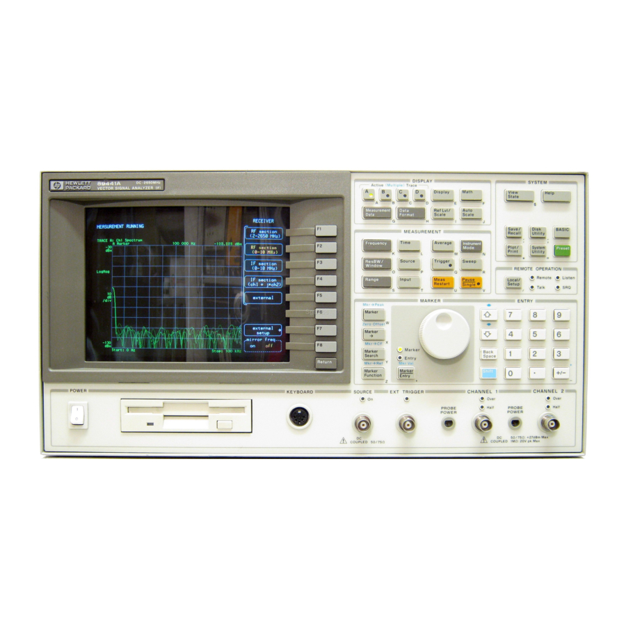
Page 3 Front Panel -A softkey’s function changes as different -Use the SYSTEM hardkeys and their menus are displayed. Its current function is menus to control various system functions determined by the video label to its left, on the (online help, plotting, presetting, and so on). analyzer’s screen.
Page 4 This page left intentionally blank...
Page 5 Failure to comply with these precautions or with specific warnings elsewhere in this manual violates safety standards of design, manufacture, and intended use of the instrument. Agilent Technologies, Inc. assumes no liability for the customer’s failure to comply with these requirements.
Page 6 FUSES Only fuses with the required rated current, voltage, and specified type (normal blow, time delay, etc.) should be used. Do not use repaired fuses or short-circuited fuse holders. To do so could cause a shock or fire hazard. DO NOT OPERATE IN AN EXPLOSIVE ATMOSPHERE Do not operate the instrument in the presence of flammable gases or fumes.
Page 7 Safety Symbols Warning, risk of electric shock Caution, refer to accompanying documents Alternating current Both direct and alternating current Earth (ground) terminal Protective earth (ground) terminal Frame or chassis terminal Terminal is at earth potential. Standby (supply). Units with this symbol are not completely disconnected from ac mains when this switch is off...
Page 8 This page left intentally blank. viii...
Page 9 89410A, order 89410U followed by the option number. To convert your 89410A DC-10 MHz Vector Signal Analyzer to an 89441A DC-2650 MHz Vector Signal Analyzer, order an 89431A. To order an option when converting your 89410A to an 89441A, order 89431A followed by the option number. IMPORTANT To convert older HP 89410A analyzers (serial numbers below 3416A00617), contact your nearest Agilent Technologies sales and service office.
Page 10 (see title page in manual) Operator’s Guide Agilent Technologies 89410A Getting (see title page in manual) Started Guide Agilent Technologies 89410A Installation and Verification Guide (see title page in manual) Agilent Technologies 89400-Series GPIB Command Reference (see title page in manual) GPIB Programmer’s Guide...
Page 11 The accessories listed in the following table are available for the Agilent 89410A. Available Accessories Part Number Agilent 89411A 21.4 MHz Down Converter Agilent 89411A 89400-Series Using Instrument BASIC Agilent 89441-90013 Instrument BASIC User’s Handbook Agilent E2083-90005 Spectrum and Network Measurements Agilent 5960-5718 Box of ten 3.5-inch double-sided, double-density disks...
Page 12 Options and Accessories: 89441A To determine if an option is installed, press [ ]. Installed System Utility option setup options are also listed on the analyzer’s rear panel. To order an option for an Agilent 89441A analyzer, order Agilent 89441U followed by the option number. Option Description Agilent 89441U Option Add Internal RF Source...
Page 13 Agilent 89410/89441A Operator’s Guide (see title page in manual) Agilent Technologies 89441A Getting Started Guide (see title page in manual) Agilent Technologies 89441A Installation and Verification Guide (see title page in manual) Agilent Technologies 89400-Series GPIB Command Reference (see title page in manual) GPIB Programmer’s Guide...
Page 14 The accessories listed in the following table are available for the Agilent 89441A. Available Accessories Part Number Agilent 89411A 21.4 MHz Down Converter Agilent 89411A 89400-Series Using Instrument BASIC Agilent 89441-90013 Instrument BASIC User’s Handbook Agilent E2083-90005 Spectrum and Network Measurements Agilent 5960-5718 Box of ten 3.5-inch double-sided, double-density disks Agilent 92192A...
Page 15 Notation Conventions Before you use this book, it is important to understand the types of keys on the front panel of the analyzer and how they are denoted in this book. Hardkeys Hardkeys are front-panel buttons whose functions are always the same. Hardkeys have a label printed directly on the key.
Page 16 This page left intentionally blank.
Page 17 In This Book This book, “Agilent 89410A/Agilent89441A Operator’s Guide”, is designed to advance your knowledge of the Agilent 89410A and Agilent 89441A Vector Signal Analyzers. You should already feel somewhat comfortable with this analyzer, either through previous use or through performing the tasks in either product’s Getting Started Guide.”...
Page 18 This page left intentionally blank. xviii...
Page 19: Table Of Contents
TABLE OF CONTENTS 1 Demodulating an Analog Signal To perform AM demodulation 1-2 To perform PM demodulation 1-4 To perform FM demodulation 1-6 2 Measuring Phase Noise To measure phase noise 2-2 Special Considerations for phase noise measurements: 2-3 3 Characterizing a Transient Signal To set up transient analysis 3-2 To analyze a transient signal with time gating 3-4 To analyze a transient signal with demodulation 3-5...
Page 20 7 Using Waterfall and Spectrogram Displays (Opt. AYB) To create a test signal 7-2 To set up and scale a waterfall display 7-4 To select a trace in a waterfall display 7-6 To use markers with waterfall displays 7-8 To use buffer search in waterfall displays 7-10 To set up a spectrogram display 7-11 To enhance spectrogram displays 7-12 To use markers with spectrogram displays 7-14...
Page 21 10 Analyzing Digitally Demodulated Signals (Options AYA and AYH) To demodulate a non-standard-format signal 10-2 To use polar markers 10-4 To view a single constellation state 10-5 To locate a specific constellation point 10-6 To use X-axis scaling and markers 10-7 To examine symbol states and error summaries 10-8 To view and change display state definitions 10-10 To view error displays 10-12...
Page 22 Calibration 15-8 16 Extending Analysis to 26.5 GHz with 20 MHz Information Bandwidth Overview 16-2 System Description 16-3 Agilent 89410A Operation 16-5 HP/Agilent 71910A Operation 16-5 Mirrored Spectrums 16-6 IBASIC Example Program 16-6 System Configuration 16-7 Agilent 89410A Configuration 16-7...
Page 23 Vector—the important details 17-7 Analog Demodulation—another view of the details 17-7 Instrument Mode? Measurement Data? Data Format? 17-8 Instrument modes 17-8 Measurement data 17-8 Data format 17-8 Unique Capabilities of the Instrument Modes 17-9 18 What Makes this Analyzer Different? Time Domain and Frequency Domain Measurements 18-2 The Y-axis (amplitude) 18-3 The X-axis (frequency) 18-3...
Page 24 Resolution bandwidth limitations 19-11 What is a detector and why is one needed 19-12 Manual sweep 19-13 Special Considerations in Vector Mode 19-14 Time data 19-15 The time record 19-16 Why is a time record needed? 19-16 Time record, span and resolution bandwidth 19-17 Measurement speed and time record length 19-17 How do the parameters interact? 19-18 Time record length limitations 19-19...
Page 25 The algorithm 20-12 Interactions with other features 20-13 Choosing trigger type with analog demodulation 20-13 Using gating and averaging with analog demodulation 20-13 Two-channel measurements and analog demodulation 20-13 21 Gating Concepts What is Time Gating? 21-2 How Does it Work? 21-4 Important Concepts 21-5 Parameter Interactions 21-6 22 Digital Demodulation Concepts (Opt.
Page 26 Filter choices for the measured and reference signals 22-17 Square-root raised cosine filters 22-18 Raised cosine filters 22-18 Gaussian filter 22-19 Low pass filter (for FSK) 22-19 User defined filters 22-19 IS-95 Filters 22-20 EDGE Filter 22-21 EDGE (winRC) Filter 22-21 23 Video Demodulation Concepts (Opt.
Page 27 24 Wideband CDMA Concepts (Options B73, B79, and 080) Overview 24-2 What you learn in this chapter 24-2 What option B73 does 24-2 What option B79 does 24-3 What option 080 does 24-3 Measurement Flow 24-4 Setting up a W-CDMA Measurement 24-6 Signal Connections and Input Range 24-6 Frequency Span 24-7 Center Frequency 24-7...
Page 29: Demodulating An Analog Signal
Demodulating an Analog Signal This chapter shows how to demodulate AM, FM, and PM signals using the Analog Demodulation instrument mode. In these examples the signals are provided by the Signals Disk which accompanies this documentation.
Page 30: To Perform Am Demodulation
Initialize the analyzer: Press [ ], [ ], then press: Instrument Mode receiver 89410A: [ input section (0-10 MHz) 89441A: [ RF section (0-10 MHz) Press [ Preset Load the source signal file AMSIG.DAT into data register D1: Insert the Signals Disk in the analyzer’s disk drive.
Page 31 Demodulating an Analog Signal Turn on AM demodulation and examine the recovered modulation signal: Press [ ], [ ] (with option AYH, press Instrument Mode Analog Demodulation ], [ ], [ ], [ demod type Analog Demodulation Return Instrument Mode Press [ ], [ ], [...
Page 32: To Perform Pm Demodulation
Initialize the analyzer: Press [ ], [ ], then press: Instrument Mode receiver 89410A: [ input section (0-10 MHz) 89441A: [ RF section (0-10 MHz) Press [ Preset Load the source signal file PMSIG.DAT into data register D2: Insert the Signals Disk in the analyzer’s disk drive.
Page 33 Demodulating an Analog Signal Turn on demodulation (PM) and examine the recovered modulation signal: Press [ ], [ ] (with option AYH, press Instrument Mode Analog Demodulation ], [ ], [ ], [ demod type Analog Demodulation Return Instrument Mode Press [ ], [ ], [...
Page 34: To Perform Fm Demodulation
Initialize the analyzer: Press [ ], [ ], then press: Instrument Mode receiver 89410A: [ input section (0-10 MHz) 89441A: [ RF section (0-10 MHz) Press [ Preset Load the source signal file PMSIG.DAT into data register D2: Insert the Signals Disk in the analyzer’s disk drive.
Page 35 Demodulating an Analog Signal Press [ ], [ ] (with option AYH, press Instrument Mode Analog Demodulation ], [ ], [ ], [ demod type Analog Demodulation Return Instrument Mode Press [ ], [ ], [ demodulation setup ch1 result Press [ ] to scale the display information.
Page 37: Measuring Phase Noise
Measuring Phase Noise This chapter demonstrates how to perform a phase noise measurement using a simulated input signal from a time capture signal.
Page 38: To Measure Phase Noise
Initialize the analyzer: Press [ ], [ ], then press: Instrument Mode receiver 89410A: [ input section (0-10 MHz) 89441A: [ RF section (0-10 MHz) Press [ Preset If your analyzer has the optional second input channel installed, turn it off:...
Page 39: Special Considerations For Phase Noise Measurements
Measuring Phase Noise Select PM demodulation: Press [ ], [ ] (with option AYH, press [ Instrument Mode Analog Demodulation Instrument ], [ ], [ ], [ demod type Analog Demodulation Return Mode Press [ ], [ ], [ demodulation setup ch1 result Select PSD measurement data: Press [...
Page 41: Characterizing A Transient Signal
Characterizing a Transient Signal This chapter demonstrates two methods of characterizing a transient signal. In this case you will characterize a simulated transmitter turn-on signal.
Page 42: To Set Up Transient Analysis
Select the baseband mode and initialize the analyzer: Press [ ], [ ], then press: Instrument Mode receiver 89410A: [ input section (0-10 MHz) 89441A: [ RF section (0-10 MHz) Press [ Preset Load the source signal file XMITR.DAT into data register D1: Insert the Signals Disk in the analyzer’s disk drive.
Page 43 Characterizing a Transient Signal Set the sweep and trigger: Press [ ], [ ], [ Trigger trigger type internal source Press [ ], [ ], [ ] to simulate a “transient.” Sweep single Pause|Single Press [ Auto Scale The display should now appear as shown below. Spectrum (top) and time domain representation (bottom) of transient signal.
Page 44: To Analyze A Transient Signal With Time Gating
Characterizing a Transient Signal To analyze a transient signal with time gating This procedure assumes that the steps in “To set up transient analysis” have been performed. If not, do so before continuing. Turn on time gating, set the gate length, and set up the knob to move the gate: Press [ ], [ ], [...
Page 45: To Analyze A Transient Signal With Demodulation
Characterizing a Transient Signal To analyze a transient signal with demodulation This procedure analyzes the frequency and amplitude variations of the transient signal with demodulation. It assumes that the steps in “To set up transient analysis” have been performed. If not, do so before beginning. If you just finished the setup procedure, go to step 2 (don’t perform this step).
Page 46 Characterizing a Transient Signal Now we’ll look at the amplitude response of the signal with AM demodulation: Press [ ], [ ], [ ], [ Instrument Mode demodulation setup ch1 result Press [ Pause|Single Now scale both traces: Press the blue [ ], [ ].
Page 47: Making On/Off Ratio Measurements
Making On/Off Ratio Measurements This chapter shows you how to measure the on/off ratio of a burst signal. This type of signal is typical in communication applications which use a burst carrier. You will use a signal from the Signals Disk to simulate a phase-modulated burst carrier.
Page 48: To Set Up Time Gating
Select the baseband mode and initialize the analyzer: Press [ ], [ ], then press: Instrument Mode receiver 89410A: [ input section (0-10 MHz) 89441A: [ RF section (0-10 MHz) Press [ Preset Load a burst signal from the Signals Disk into a register and play it through the source: Insert the Signals Disk in the internal disk drive.
Page 49 Making On/Off Ratio Measurements Turn on a second trace and configure it to display stable time data: Press [ ], [ Display 2 grids Press [ ], [ ], [ Trigger trigger type internal source Press [ Press [ ], [ Measurement Data main time ] for a 2-channel analyzer).
Page 50: To Measure The On/Off Ratio
Making On/Off Ratio Measurements To measure the on/off ratio This assumes you have already set up time gating as in “To set up time gating.” Turn on averaging: Press [ ], [ Average average on Turn on and zero the offset marker on the spectrum display: Press [ ], [ ], [...
Page 51: Making Statistical Power Measurements
Making Statistical Power Measurements This chapter shows you how to make statistical power measurements, such as CCDF (Complementary Cumulative Density Function), and peak, average, and peak-to-average statistical measurements. 5 - 1...
Page 52: To Display Ccdf
CCDF of the random noise. Preset the analyzer. Press [ ], [ ], then press: Instrument Mode receiver 89410A: [ input section (0-10 MHz) 89441A: [ RF section (0-10 MHz) Press [ Preset Select the Vector instrument mode.
Page 53 Making Statistical Power Measurements CCDF provides better resolution than CDF for low probability signals, especially when the y-axis is in log format. Presetting the analyzer automatically selects log format ([ ], [ Data Format magnitude log(dB) The analyzer plots CCDF using units of % for the y-axis and power (dB) for the x-axis.
Page 54: To Display Peak, Average, And Peak/Average Statistics
Making Statistical Power Measurements To display peak, average, and peak/average statistics This procedure shows you how to use features under [ ] to Marker Function display peak, average, and peak-to-average statistical power measurements. You can use these features to obtain the same results you get with CCDF measurements.
Page 55 Making Statistical Power Measurements Using the [ ] hardkey, the analyzer lets you set the peak Marker Function percent and then display peak, average, or peak-to-average statistical power for these configurations (otherwise the statistical softkeys are inactive): The instrument mode is not Scalar. The measurement contains time-domain data (x-axis is time).
Page 57: Creating Arbitrary Waveforms
Creating Arbitrary Waveforms This chapter shows you how to generate arbitrary waveforms using the analyzer’s arbitrary source. You can generate arbitrary waveforms that contain up to 16,384 samples of real or complex data. Under certain conditions, you can extend the arbitrary-source length to include up to 32,768 samples of real or complex data.
Page 58: To Create A Waveform Using A Single, Measured Trace
Initialize the analyzer and select the Vector instrument mode: Press [ ], [ ], then press: Instrument Mode receiver 89410A: [ input section (0-10 MHz) 89441A: [ RF section (0-10 MHz) Press [ Preset Press [...
Page 59 Creating Arbitrary Waveforms Press [ ], [ ], [ arbitrary ) , [ arb data reg], [D1 ] Source source type The analyzer’s arbitrary source is now generating the same waveform as that displayed in the original trace. The maximum number of samples in the source waveform is dependent on the sample rate used to create the arbitrary-source data.
Page 60: To Create A Waveform Using Multiple, Measured Traces
Initialize the analyzer and select the Vector instrument mode: Press [ ], [ ], then press: Instrument Mode receiver 89410A: [ input section (0-10 MHz) 89441A: [ RF section (0-10 MHz) Press [ Preset Press [ ], [...
Page 61 Creating Arbitrary Waveforms Start the measurement and view the results: Press [ ], [ Meas Restart The arbitrary source is now generating your signal. Waterfall and spectrogram displays store trace data in the trace buffer. Both displays use the same trace buffer, therefore it doesn’t matter which display you use when you save the trace buffer.
Page 62: To Create A Short Waveform Using Ascii Data
Creating Arbitrary Waveforms To create a short waveform using ASCII data There are several computer programs that let you create arbitrary waveforms (such as MATLAB or MATRIXx2 ) . This procedure shows you how to load a short, computer-generated waveform into the analyzer’s arbitrary source.
Page 63 Creating Arbitrary Waveforms The analyzer stores trace data in Standard Data Format (SDF). Therefore, you must use the Standard Data Format utilities to convert your data to the SDF format recognized by the analyzer. For details about the SDF utilities, see the Standard Data Format Utilities: User’s Guide shipped with your analyzer.
Page 64: To Create A Long Waveform Using Ascii Data
Creating Arbitrary Waveforms To create a long waveform using ASCII data There are several computer programs that let you create arbitrary waveforms (such as MATLAB or MATRIXx). This procedure shows you how to use a long, computer-generated waveform with the analyzer’s arbitrary source.
Page 65 Creating Arbitrary Waveforms Load the modified trace-buffer file into one of the analyzer’s data registers. On your computer, copy the modified trace-buffer file to floppy disk. Insert the disk in the analyzer’s disk drive. Press [ ], [ ], [ ] and select your file.
Page 66: To Create A Contiguous Waterfall Or Spectrogram Display
Creating Arbitrary Waveforms To create a contiguous waterfall or spectrogram display Contiguous traces are needed when you use a waterfall or spectrogram display to generate an arbitrary-source waveform. You use waterfall or spectrogram displays to generate arbitrary waveforms that contain more than 4096 samples of complex data or 8192 samples of real data.
Page 67 Creating Arbitrary Waveforms To learn about waterfall and spectrogram displays, see ‘’Using Waterfall And Spectrogram Displays (Opt. AYB)’’ in the Operator’s Guide and see online help for the [ ] and [ ] softkeys. waterfall setup spectrogram setup This waterfall display was created with an elevation of 25 pixels and trace height of 30 pixels.
Page 68: To Create A Fixed-Length Waterfall Display
5 ms. Substitute your values where necessary. Initialize the analyzer and select the Vector instrument mode: Press [ ], [ ], then press: Instrument Mode receiver 89410A: [ input section (0-10 MHz) 89441A: [ RF section (0-10 MHz) Press [ Preset Press [...
Page 69 Creating Arbitrary Waveforms Set the number of frequency points for your signal. The number of frequency points must be greater than the number of samples in a segment divided by 2.56 (real) or 1.28 (complex): 1920 samples = 1500 −−> Use 1601 freq. pts. For 10 segments of 1920 samples: 1.28 1600 samples...
Page 70: To Determine Number Of Samples And ∆T
Creating Arbitrary Waveforms To determine number of samples and ∆t If you are using a waterfall or spectrogram display to import data from your computer-generated waveform, the waterfall or spectrogram must have the same number of samples and ∆t as your computer-generated waveform, as explained in “To create a fixed-length waterfall display.”...
Page 71: To Output The Maximum Number Of Samples
Creating Arbitrary Waveforms To output the maximum number of samples You use time-domain data (samples) in a data register to drive the analyzer’s arbitrary source. The arbitrary source can use up to 16,384 samples. If the samples were created using a cardinal frequency span, the arbitrary source can use 32,768 samples.
Page 73: Using Waterfall And Spectrogram Displays (Opt. Ayb)
Using Waterfall and Spectrogram Displays (Opt. AYB) This chapter shows you how to view signals in an almost three dimensional way by displaying multiple traces as a function of time. 7 - 1...
Page 74: To Create A Test Signal
Preset the analyzer. Press [ ], [ ], then press: Instrument Mode receiver 89410A: [ input section (0-10 MHz) 89441A: [ RF section (0-10 MHz) Press [ Preset Select the Vector instrument mode. Press [Instrument Mode] [Vector].
Page 75 Using Waterfall and Spectrogram Displays (Opt. AYB) Hint You may want to save the current measurement state to non-volatile RAM (NVRAM). That way, if you don’t have time to finish the procedures in this chapter, you can quickly reproduce the test signal. To do this, press [Save/Recall] [default disk] [non-volatile RAM disk] [return] [save state].
Page 76: To Set Up And Scale A Waterfall Display
Using Waterfall and Spectrogram Displays (Opt. AYB) To set up and scale a waterfall display This procedure uses the signal created at the beginning of this chapter to show you how to set up and scale waterfall displays. Perform the procedure at the beginning of this chapter to create a test signal. Turn on the waterfall display for trace A.
Page 77 Using Waterfall and Spectrogram Displays (Opt. AYB) Azimuth determines the shift, or skew, of the waterfall display. Aximuth tells the analyzer how far, in pixels, to shift a trace from the previous trace. Negative numbers shift the trace left; positive numbers shift the trace right.
Page 78: To Select A Trace In A Waterfall Display
Using Waterfall and Spectrogram Displays (Opt. AYB) To select a trace in a waterfall display This procedure shows you how to select traces in a waterfall display. You can select any trace in the waterfall buffer. You can select a trace by number, or by its z-axis value.
Page 79 Using Waterfall and Spectrogram Displays (Opt. AYB) You can select a trace by number or by its z-axis value (in seconds). Trace number 1 is the first, or oldest trace in the waterfall buffer. To select a trace by its z-axis value, press [trace] followed by the z-axis value. Hint To display the current z-axis value in the [trace] softkey, press [trace] [s] .
Page 80: To Use Markers With Waterfall Displays
Using Waterfall and Spectrogram Displays (Opt. AYB) To use markers with waterfall displays This procedure uses the results of the previous procedure to show you how to use markers and offset markers with waterfall displays. Perform the previous procedure to create a waterfall display and enable trace selection.
Page 81 Using Waterfall and Spectrogram Displays (Opt. AYB) Move the marker to the next trace in the waterfall display. Press [Marker Function] followed by the up-arrow key. In this example, notice that the z-axis marker value is approximately 41.2 ms, which is the elapsed time between the two traces. In other words, 41.2 ms elapsed from when the analyzer acquired trace 2 to when it acquired trace 1.
Page 82: To Use Buffer Search In Waterfall Displays
Using Waterfall and Spectrogram Displays (Opt. AYB) To use buffer search in waterfall displays This procedure shows you how to use buffer search to do marker-search operations over all traces in the waterfall buffer. Start with step 2 if you just finished the previous procedure.
Page 83: To Set Up A Spectrogram Display
Using Waterfall and Spectrogram Displays (Opt. AYB) To set up a spectrogram display This procedure shows you how to set up and view a spectrogram display. Perform the procedure at the beginning of this chapter to create a test signal. Turn on the spectrogram display for trace A.
Page 84: To Enhance Spectrogram Displays
Using Waterfall and Spectrogram Displays (Opt. AYB) To enhance spectrogram displays This procedure shows you how to use advanced features to enhance the spectrogram display. Perform the previous procedure, “To set up a spectrogram display.” Pause the measurement after the spectrogram fills the entire display. Press [Pause|Single].
Page 85 Using Waterfall and Spectrogram Displays (Opt. AYB) Change the number of colors used in the color map. Press [return]. Press [ ] 2 [enter]. number colors Press 5 [enter]. Press 10 [enter]. Press 64 [enter] to return to the default number of colors. In this example, changing the number of colors erases the upper portion of the spectrogram display.
Page 86: To Use Markers With Spectrogram Displays
Using Waterfall and Spectrogram Displays (Opt. AYB) To use markers with spectrogram displays You use markers in a spectrogram display the same way you use markers in a waterfall display. To learn how to use markers (and select traces) in a spectrogram display, display a spectrogram instead of a waterfall and perform the following procedures: To select a trace in a waterfall display.
Page 87: To Save Waterfall And Spectrogram Displays
Using Waterfall and Spectrogram Displays (Opt. AYB) To save waterfall and spectrogram displays You save a waterfall or spectrogram display by saving the trace buffer. The trace buffer contains the traces that make up the waterfall or spectrogram display. Both waterfall and spectrogram displays share the same trace buffer (which is why you can switch between waterfall or spectrogram displays without losing data).
Page 88: To Recall Waterfall And Spectrogram Displays
Using Waterfall and Spectrogram Displays (Opt. AYB) To recall waterfall and spectrogram displays This procedure shows you how to recall waterfall and spectrogram displays. See the previous procedure for instructions on saving waterfall and spectrogram displays. Activate the trace where you want the waterfall or spectrogram display. For example, if you want to display a waterfall display in trace A, press [A].
Page 89: Using Digital Demodulation (Opt. Aya)
Using Digital Demodulation (Opt. AYA) This chapter shows you how to use digital demodulation to demodulate and view digitally modulated signals. You may perform the tasks in this chapter using signals from the Signals Disk, or you may use these tasks as a model for demodulating your own signals.
Page 90: To Prepare A Digital Demodulation Measurement
Initialize the analyzer: Press [ ], [ ], then press: Instrument Mode receiver 89410A: [ input section (0-10 MHz) 89441A: [ RF section (0-10 MHz) Press [ Preset Press [ ], [...
Page 91 Using Digital Demodulation (Opt. AYA) Set up the trigger: Press [ ], [ ], [ ], [ ], [ ], 1, [ Trigger trigger type internal source return ch1 delay This example uses a signal which has been supplied from the Signals Disk. When you supply another signal to the channel 1 input you need to select appropriate center frequency, span, range, and triggering parameters prior to demodulating the signal.
Page 92: To Demodulate A Standard-Format Signal
Using Digital Demodulation (Opt. AYA) To demodulate a standard-format signal This task shows you how to demodulate the NADC signal on the Signals Disk. Configure the analyzer for a digital demodulation measurement. If you haven’t already done so, perform the steps in the previous task, ‘’To prepare a digital demodulation measurement.’’...
Page 93: To Select Measurement And Display Features
Using Digital Demodulation (Opt. AYA) To select measurement and display features The analyzer provides many different ways of viewing demodulated data. This task shows you how to display demodulated data two different views in two grids. Demodulate your signal as shown in the previous task. Select multiple display grids: Press [ ], [...
Page 94: To Set Up Pulse Search
Using Digital Demodulation (Opt. AYA) To set up pulse search In this example you learn how to perform pulse search on a burst signal. This example uses a signal, provided on the Signals Disk, which is a record of the output of a keyed NADC radio transmission. Load “MEAS_PI4.DAT”...
Page 95 Using Digital Demodulation (Opt. AYA) Demodulating a pulsed signal 8 - 7...
Page 96: To Set Up Sync Search
Using Digital Demodulation (Opt. AYA) To set up sync search In this task you learn how to synchronize your measurement by using a specific bit pattern within the chain of bits. You learn how to define sync words and set an offset. Since sync search is often used with pulsed signals, this example assumes you have already acquired and demodulated a pulsed signal as shown in the previous task.
Page 97: To Select And Create Stored Sync Patterns
Using Digital Demodulation (Opt. AYA) To select and create stored sync patterns When using sync search you can enter a sync bit pattern as in the previous task, or you can load up to six of your own sync patterns into softkeys F3 through F8 and then use the softkeys to select a sync bit pattern.
Page 98: To Demodulate And Analyze An Edge Signal
Option B7A must be installed to demodulate EDGE signals. Initialize the analyzer: Press [ ], [ ], then press: Instrument Mode receiver 89410A: [ input section (0-10 MHz) 89441A: [ RF section (0-10 MHz) Press [ Preset Connect your EDGE signal to the channel 1 INPUT.
Page 99 Using Digital Demodulation (Opt. AYA) Display the ideal vector diagram in trace C and compare it to trace A: Press [ ], [ ], [ IQ reference time Measurement Data Press [ ], [ Data Format polar IQ vector Press [ ], [ more format setup symbol dots...
Page 100: To Troubleshoot An Edge Signal
Using Digital Demodulation (Opt. AYA) To troubleshoot an EDGE signal This task shows you how to use the error-vector trace and the symbol table to diagnose problems with an EDGE signal. To simulate an error condition, the task uses the analyzer’s source to mix a 5.1 MHz, –35 dbM sine wave with the EDGE signal loaded in the previous task.
Page 101 Using Digital Demodulation (Opt. AYA) Mag Err and Phase Err are especially useful to determine if your signal contains AM, PM, spurious, or excessive noise errors. AM errors increase Mag Err; PM errors increase Phase Err; spurious and noise errors increase both Mag Err and Phase Err.
Page 102: To Demodulate And Analyze An Msk Signal
Using Digital Demodulation (Opt. AYA) To demodulate and analyze an MSK signal This example uses an MSK signal from the Signals Disk to show you how to demodulate an MSK signal and view MSK phase transitions. Load “MSK.DAT” from the Signals Disk into the arbitrary source: Perform steps 1, 2, and 3 in ‘’To prepare a digital demodulation measurement.’’...
Page 103 Using Digital Demodulation (Opt. AYA) Format traces B and D to view the reference versus the measured trellis diagram: Press [ ], [ ], [ ], [ Display 2 grids view/overlay traces D on Press [ ], [ ], [ Measurement Data IQ reference time Press [...
Page 104: To Demodulate A Two-Channel I/Q Signal
] key. Trigger Proceed with digital demodulation as shown previously. For more information on this type of measurement see online help for the [input section (ch1 + j*ch2)] (89410A) or [IF section (ch1 + j*ch2)] (89441A) key. 8 - 16...
Page 105: Using Video Demodulation (Opt. Ayh)
Using Video Demodulation (Opt. AYH) This chapter shows you how to use digital video demodulation to demodulate and view digitally-modulated video signals. You may perform the tasks in this chapter using signals from the Signals Disk, or you may use these tasks as a model for demodulating your own signals. 9 - 1...
Page 106: To Prepare A Vsb Measurement
If you have your own 8 VSB signal, use the steps below and enter the demodulation parameters for your signal. Initialize the analyzer: Press [ ], [ ], then press: Instrument Mode receiver 89410A: [ input section (0-10 MHz) 89441A: [ RF section (0-10 MHz) Press [ Preset Press [ ], [...
Page 107 Using Video Demodulation (Opt. AYH) VSB measurements typically require a large portion of measurement memory. Therefore, it is a good idea to choose the maximum value (4096) for [ ] (see step 1). For details about [ ], see online max time points max time points help (press [...
Page 108: To Determine The Center Frequency For A Vsb Signal
Initialize the analyzer: Press [ ], [ ], then press: Instrument Mode receiver 89410A: [ input section (0-10 MHz) 89441A: [ RF section (0-10 MHz) Press [ Preset Press [ ], [...
Page 109 Using Video Demodulation (Opt. AYH) Set the center frequency to the computed value: Press [ ], [ ], 6 [ center MHz) Frequency Note If your pilot is on the high (right) side of the spectrum, you must configure the analyzer to demodulate a high-side pilot.
Page 110: To Demodulate A Vsb Signal
Using Video Demodulation (Opt. AYH) To demodulate a VSB signal This task shows you how to demodulate a VSB signal. The task uses the 8 VSB time-capture signal that you loaded into the analyzer in ‘’To prepare a VSB measurement’’. Prepare the analyzer for a VSB measurement as shown in the ‘’To prepare a VSB measurement’’.
Page 111 Using Video Demodulation (Opt. AYH) View the constellation and eye diagram: Press [ ], [ Display 2 grids Press [ ], [ ], [ Measurement Data IQ measured time Press [ ], [ Data Format polar (IQ) constellation Press [ ], [ ], [ Measurement Data...
Page 112: To Prepare A Qam Or Dvb Qam Measurement
Initialize the analyzer: Press [ ], [ ], then press: Instrument Mode receiver 89410A: [ input section (0-10 MHz) 89441A: [ RF section (0-10 MHz) Press [ Preset Press [ ], [...
Page 113 Using Video Demodulation (Opt. AYH) Set up the trigger: Press [ ], [ ], [ ], [ ], [ ], 3, [ Trigger trigger type internal source return ch1 delay This example uses the 32 DVB QAM signal from the Signals Disk. This signal was generated following a procedure similar to that shown in chapter 9, ‘’To create an ideal digitally modulated signal.’’...
Page 114: To Demodulate A Qam Or Dvb Qam Signal
Using Video Demodulation (Opt. AYH) To demodulate a QAM or DVB QAM signal This task shows you how to demodulate the 32 DVB QAM signal generated in ‘’To prepare a QAM or DVB QAM measurement’’. Prior to demodulating a video signal you must select the correct center frequency, frequency span, and range as shown in that task.
Page 115 Using Video Demodulation (Opt. AYH) Hint You use ] to set demodulation parameters, you use [demodulation setup ] to select the measurement calculation used on demodulated Measurement Data data, and you use [ ] to select a display format (trace coordinates). To Data Format learn more about these keys and the choices under them, see online help.
Page 116: To Select Measurement And Display Features
Using Video Demodulation (Opt. AYH) To select measurement and display features You can display demodulated data in many different formats. This task uses the demodulated 32 DVB QAM signal from the previous task to show you just a few ways of viewing demodulated data. Select multiple display grids: Press [ ], [...
Page 117: To Set Up Sync Search (Qam Only)
Using Video Demodulation (Opt. AYH) To set up sync search (QAM only) In this task you learn how to synchronize your measurement by using a specific bit pattern within the chain of bits. You learn how to define sync words and set an offset. Sync search operates the same for both digital and video demodulation.
Page 118: To Select And Create Stored Sync Patterns (Qam Only)
Using Video Demodulation (Opt. AYH) To select and create stored sync patterns (QAM only) When using sync search you can enter a sync bit pattern as in the previous task, or you can load up to six of your own sync patterns into softkeys F3 through F8, and then use the softkeys to select a sync bit pattern.
Page 119: To Demodulate A Two-Channel I/Q Signal
] key. Trigger Proceed with digital demodulation as shown previously. For more information on this type of measurement see online help for the ] (89410A) or [ (89441A) key. input section (ch1 + j*ch2) IF section (ch1 + j*ch2) 9 - 15...
Page 121: Analyzing Digitally Demodulated Signals (Options Aya And Ayh)
Analyzing Digitally Demodulated Signals (Options AYA and AYH) This chapter shows you how to analyze signals demodulated with Digital Demodulation or with Video Demodulation. The tasks in this chapter use digital demodulation, but the same steps apply to video demodulation. You will learn how to select measurement data and compatible data formats, use polar markers, examine symbol tables, display state definitions, and examine errors.
Page 122: To Demodulate A Non-Standard-Format Signal
Demodulation Concepts (Opt. AYH) chapter explains how video demodulation differs from digital demodulation. Initialize the analyzer: Press [ ], [ ], then press: Instrument Mode receiver 89410A: [ input section (0-10 MHz) 89441A: [ RF section (0-10 MHz) Press [ Preset Press [ ], [...
Page 123 Analyzing Digitally Demodulated Signals (Options AYA and AYH) Choose demodulation setup parameters: Press [ ], [ ], [ Time pulse search off sync search off Press [ ], 5, [ points/symbol enter Press [ ], [ ], [ ], [ Instrument Mode demodulation setup demod format...
Page 124: To Use Polar Markers
Analyzing Digitally Demodulated Signals (Options AYA and AYH) To use polar markers This task shows you how to select the polar-marker format (magnitude and phase or real and imaginary) and polar-marker units (dBm, Watts, or volts). This task is a continuation of the previous task. Select result coordinate power calculation: Press [ ], [demodulation setup], [more], [...
Page 125: To View A Single Constellation State
Analyzing Digitally Demodulated Signals (Options AYA and AYH) To view a single constellation state In this task you use the marker as a reference to reposition a constellation state to the center of the screen and zoom in. This task is a continuation of the previous task.
Page 126: To Locate A Specific Constellation Point
Analyzing Digitally Demodulated Signals (Options AYA and AYH) To locate a specific constellation point You now use the offset marker as a pointer to snap the main marker to a constellation point. This is more convenient than searching linearly through time in order to position the main marker on a desired constellation point.
Page 127: To Use X-Axis Scaling And Markers
Analyzing Digitally Demodulated Signals (Options AYA and AYH) To use X-axis scaling and markers This task shows you how to zoom-in on a selected portion of the x-axis. This task is a continuation of the previous task. Select both A and B as active traces: Press [ ], [ Display...
Page 128: To Examine Symbol States And Error Summaries
Analyzing Digitally Demodulated Signals (Options AYA and AYH) To examine symbol states and error summaries This task shows you how to display the symbol table, which contains demodulated bits and numeric error information. This task also shows you how to couple the marker in the symbol table to the constellation diagram so you can see the bits that correspond to a state.
Page 129 Analyzing Digitally Demodulated Signals (Options AYA and AYH) A Marker 3.00000 sym 15.000 = 859.14 m%rms 1.4978 % pk at sym MagErr = 609.17 m%rms 1.4317 % pk at sym Phase Err = 623.96 mdeg 2.1174 deg pk at sym Freq Err = 1.7722 IQ Offset = -66.106...
Page 130: To View And Change Display State Definitions
Analyzing Digitally Demodulated Signals (Options AYA and AYH) To view and change display state definitions This task shows you how to view and change the state definitions corresponding to the detection decision points (symbol locations). You can view and change state definitions for most modulation formats. This task is a continuation of the previous task.
Page 131 Analyzing Digitally Demodulated Signals (Options AYA and AYH) Note Note that for video demodulation (option AYH), you cannot display or change the state definitions for DVB QAM. State definitions for DVB QAM are fixed as defined in the European Telecommunication Standard (online help for the ] softkey shows the state definitions as defined in this standard).
Page 132: To View Error Displays
Analyzing Digitally Demodulated Signals (Options AYA and AYH) To view error displays This task shows you how to view several different error displays, such as the error-vector magnitude (EVM), magnitude error, and phase error at each symbol point. This task is a continuation of the previous task. Select four grids: Press [ ], [...
Page 133: Creating User-Defined Signals (Options Aya And Ayh)
Creating User-defined Signals (Options AYA and AYH) This chapter shows you how to create your own digitally modulated signals. 11 - 1...
Page 134: To Create An Ideal Digitally Modulated Signal
3. Initialize the analyzer: Press [ ], [ ], then press: Instrument Mode receiver 89410A: [ input section (0-10 MHz) 89441A: [ RF section (0-10 MHz) Press [ Preset Press [ ], [...
Page 135 Creating User-defined Signals (Options AYA and AYH) You may use the analyzer to create custom arbitrary waveforms corresponding to digital communication signals. Since the I/Q reference signal is the ideal representation of a format type, a properly saved version of the reference signal provides an ideal waveform. The internally generated waveforms may be used as test signals (to test an amplifier, for example).
Page 136: To Check A Created Signal
Creating User-defined Signals (Options AYA and AYH) To check a created signal This section assumes you have created a signal as shown on the previous page, have not changed any setup parameters, and have not preset the instrument. This task uses digital demodulation. If you want to perform this task using video demodulation, choose video demodulation instead of digital demodulation in step 4.
Page 137 Creating User-defined Signals (Options AYA and AYH) Format both traces simultaneously: Press [ ], [ ], [ ], [ Shift Data Format polar IQ constellation Press [ ], [ more format setup symbol dots Press [ Auto Scale Be careful when selecting a reference filter if the demodulation format uses distributed filtering.
Page 138: To Create A User-Defined Filter
Creating User-defined Signals (Options AYA and AYH) To create a user-defined filter This task shows you how to create filters that you can use as the measured or reference filter. This task uses digital demodulation. If you want to perform this task using video demodulation, choose video demodulation instead of digital demodulation in step 4.
Page 139 Creating User-defined Signals (Options AYA and AYH) The trace display of “GAUSS1.DAT”. 11 - 7...
Page 141: Using Adaptive Equalization (Options Aya And Ayh)
Using Adaptive Equalization (Options AYA and AYH) This section shows you how to use Adaptive Equalization. Adaptive equalization removes linear errors from modulated signals by dynamically creating and applying a compensating filter. Adaptive equalization is only available in Digital and Video Demodulation instrument modes. 12-1...
Page 142: To Determine If Your Analyzer Has Adaptive Equalization
If your analyzer does not have all of the above options and hardware, you must purchase the options or hardware that you are missing. To do this, contact your Agilent Technologies sales representative or your local Agilent Technologies Sales and Service office (listed on the inside, rear cover of the Operator’s Guide).
Page 143: To Load The Multi-Path Signal From The Signals Disk
Initialize the analyzer and select the Digital Demodulation instrument mode: Press [ ], [ ], then press: Instrument Mode receiver 89410A: [ input section (0-10 MHz) 89441A: [ RF section (0-10 MHz) Press [ Preset Press [...
Page 144: To Demodulate The Multi-Path Signal
Using Adaptive Equalization (Options AYA and AYH) To demodulate the multi-path signal This task shows you how to demodulate the multi-path signal that you loaded in the previous task. Load the multi-path signal as instructed in the previous task. Set demodulation parameters for this signal: Press [ ], [ Instrument Mode...
Page 145 Using Adaptive Equalization (Options AYA and AYH) In this example, traces A and B show the default frequency response and impulse response of the equalization filter. By default, the equalization filter has a unit impulse response. This signal is difficult to demodulate due to linear distortion.
Page 146: To Apply Adaptive Equalization
Using Adaptive Equalization (Options AYA and AYH) To apply adaptive equalization This task shows you how to apply adaptive equalization to the multi-path signal that you demodulated in the previous task. Perform the previous task. Display the equalization-filter menu: Press [ ], [ ], [ more...
Page 147 Using Adaptive Equalization (Options AYA and AYH) The [ ] determines how quickly the old and new filter-coefficients convergence converge. Larger values converge faster. Values that are too large can cause the adaptation algorithm to become unstable or fluctuate from stable to unstable.
Page 148: To Measure Signal Paths
Using Adaptive Equalization (Options AYA and AYH) To measure signal paths This task shows you how to use the equalization filter’s impulse response to identify and measure paths in a multi-path signal. This task uses the multi-path signal on the Signals Disk and is a continuation of the previous task.
Page 149 Using Adaptive Equalization (Options AYA and AYH) Each point in the impulse-response display corresponds to a tap in the feed-forward equalizer (FFE). In a FFE, large coefficients that are separate from the main tap correspond directly to alternate signal paths. The smaller peaks are a result of the same alternate signal paths that created the large peaks.
Page 150: To Learn More About Equalization
Using Adaptive Equalization (Options AYA and AYH) To learn more about equalization Adaptive equalization is a powerful feature that you can use in many applications. The following paragraphs include additional information that may help you use adaptive equalization for your application. Equalization is available only for Digital and Video Demodulation instrument modes.
Page 151: Using Wideband Cdma (Options B73, B79, And 080)
Using Wideband CDMA (Options B73, B79, and 080) This chapter shows you how to make Wideband CDMA measurements. For a conceptual overview of Wideband CDMA, see the chapter titled Wideband CDMA Concepts. 13 - 1...
Page 152: To View A W-Cdma Signal
Using Wideband CDMA (Options B73, B79, and 080) To view a W-CDMA signal All tasks in this chapter were created using a 3GPP 1999 forward-link signal (option 080). The signal was generated with an HP/Agilent E4433 ESG Signal Generator at 5 MHz, –10 dBm, and using the channel definitions shown below.
Page 153 Connect your signal to the Channel 1 input. Initialize the analyzer and select the Vector instrument mode: Press [ ], [ ], then press: Instrument Mode receiver 89410A: [ input section (0-10 MHz) 89441A: [ RF section (0-10 MHz) Press [ Preset Press [...
Page 154: To Demodulate A W-Cdma Signal
Using Wideband CDMA (Options B73, B79, and 080) To demodulate a W-CDMA signal This task shows you how to demodulate the W-CDMA signal that you loaded in the previous task. If you are using your own W-CDMA signal instead of the one from the previous task, you may need to change some of the parameters set in step 5 to match those of your signal.
Page 155 Using Wideband CDMA (Options B73, B79, and 080) One important parameter set by this procedure is the maximum W-CDMA span. This parameter allocates memory for W-CDMA measurements. Since W-CDMA measurements require large amounts of memory, set this parameter to the smallest frequency span that you will measure. If the analyzer is unable to lock to your signal, verify that you are using the correct chip rate, scramble code, and center frequency.
Page 156: To View Data For A Single Code Layer
Using Wideband CDMA (Options B73, B79, and 080) To view data for a single code layer This task builds on the previous task to show you how to view code-domain power for a single code layer. Single code-layer displays are useful if the composite display does not accurately identify which layer a channel resides in.
Page 157 Using Wideband CDMA (Options B73, B79, and 080) Trace B shows code-domain power for a single code layer: code layer C6 (60 ksym/s). This code layer has 64 code channels (codes 0 to 63 on the x-axis). Channels that are active in this code layer are colored.
Page 158: To View Data For A Single Code Channel
Using Wideband CDMA (Options B73, B79, and 080) To view data for a single code channel This task builds on the previous task to show you how to view the vector diagram for individual channels. The power varies in each channel. The task turns normalization off so you can see the vector diagram change size when you change channels.
Page 159 Using Wideband CDMA (Options B73, B79, and 080) mkr → layer/channel The beginning steps show you how to use the [ ] softkey Marker → (under [ ]). The final step shows you how to use the [ code channel ] mkr →...
Page 160: To View Data For One Or More Slots
Using Wideband CDMA (Options B73, B79, and 080) To view data for one or more slots This task builds on the previous task to show you how to use time gating. Time gating lets you view measurement data for selected slots. Perform the previous task.
Page 161 Using Wideband CDMA (Options B73, B79, and 080) Tip 1 You do not have to start a new measurement when you use time gating. You can change the gate length and gate delay to see different gated results on the same measurement data.
Page 162: To View The Symbol Table And Error Parameters
Using Wideband CDMA (Options B73, B79, and 080) To view the symbol table and error parameters This task builds on the previous task to show you how to use the symbol table. Perform the previous task. Display the symbol table for the gated results in trace A: Press [ Press [ ], [...
Page 163 Using Wideband CDMA (Options B73, B79, and 080) The symbol table and error summary information for slot 2, code layer 5, channel 9. Symbol Table/Error Summary results for C5 (9), slot two 13 - 13...
Page 164: To Use X-Scale Markers On Code-Domain Power Displays
Using Wideband CDMA (Options B73, B79, and 080) To use x-scale markers on code-domain power displays This task builds on the previous task to show you how to use x-scale markers to ‘’zoom’’ in on channels in a code-domain power display. Demodulate the W-CDMA signal as shown earlier in this chapter.
Page 165: Using The Lan (Options Uth & Ug7)
Using the LAN (Options UTH & UG7) The tasks in this section show you how to configure and use the analyzer’s optional LAN interface. The LAN interface is present only in analyzers that have option UTH. X-Windows operation and FTP (File Transfer Protocol) are available only in analyzers that have option UG7 (Advance LAN).
Page 166: To Determine If You Have Options Uth And Ug7
Option UG7 also includes FTP (File Transfer Protocol) software. You can use FTP to transfer data to and from the analyzer. To order options, contact your local Agilent Technologies Sales and Service Office. 14 - 2...
Page 167: To Connect The Analyzer To A Network
ThinLAN network. However, the AUI Port lets you to connect the analyzer to ThinLan, ThickLAN, or StarLAN 10 networks via the appropriate off-board MAU. (These networks are Agilent Technologies’s implementation of IEEE 802.3 types 10BASE2, 10BASE5, and 10BASE-T.) The analyzer should be connected to a network by only one of its LAN connectors.
Page 168: To Set The Analyzer's Network Address
Using the LAN (Options UTH & UG7) To set the analyzer’s network address Ask your network administrator to assign an Internet Protocol (IP) address to your analyzer. Write down the address for use in step 4. If your analyzer must communicate with computers outside of the local subnet, ask your network administrator for the IP address and subnet mask required to route data through the local gateway.
Page 169: To Activate The Analyzer's Network Interface
Using the LAN (Options UTH & UG7) To activate the analyzer’s network interface Press [ ], [ ], then press [ ] to display “active.” Local/Setup LAN setup LAN power-on Turn off the analyzer, then turn it back on to make the new setting permanent. When you are not using the network interface, you should press ] to display “inactive.”...
Page 170: To Send Gpib Commands To The Analyzer
Using the LAN (Options UTH & UG7) To send GPIB commands to the analyzer Confirm that the first four tasks in this chapter have been completed. If you do not know the network address of your analyzer, press [ Local/Setup ], [ ], then write down the value displayed under [ LAN setup...
Page 171: To Select The Remote X-Windows Server
Using the LAN (Options UTH & UG7) To select the remote X-Windows server Determine the IP address of the computer you will use for remote X-Windows operation. (Ask your network administrator for help if you don’t know how to do this.) Write down the address for use in step 3. Press [ ], [ Local/Setup...
Page 172: To Initiate Remote X-Windows Operation
Using the LAN (Options UTH & UG7) To initiate remote X-Windows operation Confirm that the previous six tasks have been completed. On the remote computer (selected in the previous task), position the mouse pointer in one of the windows, then enter the following command: xhost + On the analyzer, press [ ], [ Local/Setup...
Page 173: To Use The Remote X-Windows Display
Using the LAN (Options UTH & UG7) To use the remote X-Windows display Confirm that the previous task has been completed. Use the instructions in the following paragraphs to control the analyzer from the remote X-Windows display. To press a key. Place the cursor on the key, then click the left mouse button. To activate shifted key functions.
Page 174: To Transfer Files Via The Network
Using the LAN (Options UTH & UG7) To transfer files via the network Confirm that the first four tasks in this chapter have been completed. If you do not know the network address of your analyzer, press [ Local/Setup ], [ ], then write down the value displayed under [ LAN setup LAN port setup...
Page 175: Using The Agilent 89411A Downconverter
Using the Agilent 89411A Downconverter The 89411A allows the use of the advanced analysis features of the 89410A (the IF Section) to be applied to signals above the frequency limit of the 89441A. 15-1...
Page 176 The Agilent 89411A at a Glance Agilent 89411A front panel Agilent 89411 rear panel Agilent 89411A block diagram 15-2...
Page 177 The 89411A is a fixed downconverter used to translate the 21.4 MHz IF output on several Agilent Technologies RF/microwave spectrum analyzers to a baseband frequency within the range of the 89410A. It translates the entire IF bandwidth to a baseband frequency centered at 5.6 MHz, The conversion gain of the 89411A can be varied to be compatible with several different spectrum analyzers.
Page 178: Connection And Setup Details For The Agilent 89411A
Using the Agilent 89411A Downconverter Connection and setup details for the Agilent 89411A 89410A 89411A RF or microwave spectrum analyzer Agilent 89411 setup diagram 15-4...
Page 179 89410. Its level is nominally −15 dBm when the step attenuator in the 89411A is set to the rightmost position (labeled +5 dB). For optimum results the input range of the 89410A should be set to −14 dBm. Note...
Page 180 Using the Agilent 89411A Downconverter If the RF/microwave analyzer is an MMS system: Several possibilities exist here, depending on the combination of RF and IF modules present. In addition, the frequency reference connections are more involved. The conversion gain of the system depends on which IF module supplies the 21.4 MHz IF signal, and the attenuator setting of the RF section.
Page 181 Using the Agilent 89411A Downconverter In some of the situations listed above, the combination of input signal level, attenuation, and IF section employed may result in a IF level at the 89411 input which is too large. The conversion gain switch on the rear of the 89411A should be set to provide a lower amount of conversion gain in this case.
Page 182: Calibration
Take the cable which would normally be connected from the 89411A output to the 89410A channel 1 input and connect it from the 89410A source to the channel 1 input instead. Set up the 89410A as follows: Initialize the analyzer. Press [ Preset Set up the IF parameters.
Page 183 Using the Agilent 89411A Downconverter Press [ ] 22 [ ] (appropriate for the HP/Agilent 8566A/B). maximum freq To enable control of the external spectrum analyzer via GPIB: rcvr control on] Press [ Press [ ], [ ], [ ], [ ], 18, [ system controller peripheral addresses...
Page 184 Set the display scale to linear and adjust the reference level to −22 dBm. Turn averaging off: Press ], [ average off Average The source signal now appears on the 89410A screen. Press [ ], [ ], [ ], [ ], [/], [ ], [...
Page 185 Agilent 89411A correction data Set the Measurement Data back to the function (F5) containing SPEC1/D1. Now the screen displays the 89410A source signal with any frequency response contributions of the RF/microware analyzer and the 89411A removed. This procedure does not correct for RF unflatness contributed by the RF/microwave analyzer, only IF effects are corrected.
Page 187: Extending Analysis To 26.5 Ghz With 20 Mhz Information Bandwidth
Extending Analysis to 26.5 GHz with 20 MHz Information Bandwidth This chapter shows you how to use the HP/Agilent 71910A wideband receiver to extend the frequency coverage and information bandwidth of an Agilent 89400-series vector signal analyzer. Information in this chapter is from Product Note 89400-13.
Page 188: Overview
7 MHz bandwidth and that may exist only at microwave frequencies. By combining two products—the Agilent 89410A vector signal analyzer and the HP/Agilent 71910A wideband receiver into a single measurement system—the unique capabilities of the vector signal analyzer can be used on signals with 20 MHz bandwidth at frequencies up to 26.5 GHz.
Page 189: System Description
IF and quadrature outputs. Note The 89441A consists of an 89410A (the IF section) and an 89431A (the RF section). To use an 89441A with the 71910A, disconnect the RF section and connect the IF section to the 71910A as described in this chapter.
Page 190 Extending Analysis to 26.5 GHz with 20 MHz Information Bandwidth Simplified System Block Diagram 16 - 4...
Page 191: Agilent 89410A Operation
10 MHz. Normally, this would represent the maximum bandwidth of the signal to be analyzed. However, the 89410A is capable of treating the signals on each channel as two parts of the same signal. That is, the signal going into channel one represents the real part of a complex signal, and the signal going into channel two represents the imaginary part.
Page 192: Mirrored Spectrums
IQ demodulation. The gain of the IF section is set so that the IQ demodulator operates over a signal level range where it is most linear. The IF gain resolution is 1 dB. The 89410A input range is set to be compatible with the the full-scale output of the IQ demodulator.
Page 193: System Configuration
89410A, the display may not be necessary. If however you are interested in making scalar spectrum measurements over a range of frequencies wider than the capabilities of the 89410A (20 MHz), or you intend to use other spectrum measurement capabilities provided by the 71910A system, then your system must include the display.
Page 194: Hp/Agilent 71910A Configuration
Extending Analysis to 26.5 GHz with 20 MHz Information Bandwidth HP/Agilent 71910A Configuration The 71910A receiver contains all the Modular Measurement System (MMS) components which make wideband vector signal analysis possible. Minimally, Option 004 (Analog I/Q Outputs) must be ordered and, depending on the other measurements you may want to make with the system, the MMS display (70004A) may also be needed.
Page 195 Extending Analysis to 26.5 GHz with 20 MHz Information Bandwidth Recommended Configuration Agilent 89410A Vector Signal Analyzer (must be firmware revision A.04.00 or greater) Option AY7 Second 10 MHz input channel Option AYA Vector Modulation Analysis Option 1C2 Instrument BASIC (includes the example program described earlier in this chapter) HP/Agilent 71910A Wideband Receiver (must be instrument firmware revision 94120 (B.05.00) or greater;...
Page 196: System Connections
If your 89410A includes Option UFG or UTH, you have a second GPIB connector. Referring to either figure, note that the GPIB connection is made from the main GPIB port of the 89410A (labeled GPIB) and not the connector labeled System Interconnect.
Page 197 Extending Analysis to 26.5 GHz with 20 MHz Information Bandwidth Front panel connections Rear panel connections HP 89410A HP 70004A Display Section HP 71910A Option 004 HP 70001A Mainframe System With the HP/Agilent 70004A Display 16 - 11...
Page 198 70310A Precision Reference 100 MHz 70900B LO Module 100 MHz IN Module 10 MHz 89410A EXT REF IN Additional connections needed when the system is configured with the 70004A display and the 70902A and 70903A IF Modules. 70902A IF Module VIDEO OUT...
Page 199: Operation
Operation The vector signal analyzer provides for all signal processing, display and analysis. With the exception of scalar analysis, all 89410A features are available in the wideband vector signal analyzer system. The example program only needs to provide control over center frequency, input attenuation, spectral mirroring and system calibration.
Page 200: Controlling The Receiver
These functions take care of setting the 71910A center frequency, updating the annotation on the 89410A, and mirroring the spectrum display if necessary. Setting the Mirror Frequency Key Another important function that the example program handles is the setting of the mirror frequency key, used to flip or invert the spectrum of the signal about zero hertz.
Page 201 Extending Analysis to 26.5 GHz with 20 MHz Information Bandwidth With two instruments, there are actually two sets of input attenuators that need to be adjusted. Obviously, the input to the microwave receiver is adjusted based on the level of the signal to be measured. The vector signal analyzer inputs are adjusted to reflect the I and Q signal levels at the output of the IF module.
Page 202: Resolution Bandwidth
DC offset and LO (local oscillator) feedthrough will cause a residual response at the center of the screen. The contribution of the 89410A to this response is from DC offset in it’s input circuits. This term is measured and removed on a periodic basis automatically by the 89410A unless you explicitly disable this ‘Auto-zero’...
Page 203: Calibrating The System
Extending Analysis to 26.5 GHz with 20 MHz Information Bandwidth Calibrating the System The system calibration described earlier is very easy to perform using the example program. Once the instruments are properly connected, the example program is started—automatically configuring the instruments for wideband vector signal analysis.
Page 204: Calibration Methods
Extending Analysis to 26.5 GHz with 20 MHz Information Bandwidth Calibration Methods The 89410A vector signal analyzer and the 71910A receiver are both capable of self calibration. To obtain the best system performance, the instruments must be calibrated together. The IBASIC example program calibrates both instruments as a system. The program compensates for system-induced errors, such as unequal cable lengths for the I and Q signals.
Page 205: Dc Offset
I channel. The same procedure is also performed on the Q channel. At the start of the DC offset calibration, the example program instructs the 89410A to perform an internal offset calibration. This calibration removes DC from the vector signal analyzer inputs without consideration of the input signal.
Page 206: Channel Match
Extending Analysis to 26.5 GHz with 20 MHz Information Bandwidth Channel Match Channel match is also important for preserving the dynamic range of the measurement. System errors that cause mismatch include gain imbalance, delay mismatch and frequency response differences between the I and Q signals.
Page 207 Extending Analysis to 26.5 GHz with 20 MHz Information Bandwidth The square root of the average magnitude squared is used to set the overall gain adjustment. This minimizes the absolute error across the 20 MHz bandwidth rather than the error at the center frequency. The average ratio is used to determine the gain mismatch.
Page 208: Quadrature
Extending Analysis to 26.5 GHz with 20 MHz Information Bandwidth Quadrature The final calibration is for quadrature error. Although a value for quadrature error was obtained in the channel match calibration, the number cannot be used by itself to set the quadrature adjustment DAC in the IF module as the mapping from DAC setting to phase is not known.
Page 209: Choosing An Instrument Mode
Choosing an Instrument Mode The analyzer provides three instrument modes—Scalar, Vector, and Analog Demodulation. This chapter provides a brief overview of these instrument modes and guidelines for choosing the best one. You can also order additional, optional instrument modes—for details, see these chapters: Digital Demodulation Concepts, Video Demodulation Concepts, and Wideband CDMA Concepts.
Page 210: Why Use Scalar Mode
Choosing an Instrument Mode Why Use Scalar Mode? If you’ve used a spectrum analyzer before, you should have no trouble making scalar measurements with this analyzer. And even if you haven’t used a spectrum analyzer before, you’ll find this analyzer quite easy to learn. Scalar measurements are implemented differently than measurements in the traditional swept-tuned spectrum analyzer, but the results will appear familiar to you.
Page 211 Choosing an Instrument Mode Measurement data flow diagram for Scalar Mode 17 - 3...
Page 212: Why Use Vector Mode
100 kHz. But in this analyzer, Vector Mode lets you perform FFT measurements up to 10 MHz for the Agilent 89410A and beyond 1 GHz for the Agilent 89441A. Use Vector Mode when you need:...
Page 213 Choosing an Instrument Mode Measurement data flow diagram for Vector Mode 17 - 5...
Page 214: Why Use Analog Demodulation Mode
Choosing an Instrument Mode Why Use Analog Demodulation Mode? The best way to make many measurements often includes the ability to characterize the amplitude, frequency, and phase relationships between signal components. Analog Demodulation mode provides this capability. For additional details on this mode see “Analog Demodulation Concepts” later in this book. Analog demodulation is derived from Vector Mode.
Page 215: The Advantage Of Using Multiple Modes
Choosing an Instrument Mode The Advantage of Using Multiple Modes You can often take advantage of the analyzer’s flexibility by using more than one instrument mode in a measurement scenario. Scalar—the big picture Use Scalar Mode to identify signals present in a wide span and to evaluate small signals very close to the noise floor.
Page 216: Instrument Mode? Measurement Data? Data Format
Choosing an Instrument Mode Instrument Mode? Measurement Data? Data Format? Instrument modes When you specify an instrument mode, you are asking the analyzer to acquire input data and process it in a certain way. For example, with the Vector Mode, the analyzer uses an FFT algorithm to convert a single time record into the most basic frequency domain measurement available—the spectrum.
Page 217: Unique Capabilities Of The Instrument Modes
Choosing an Instrument Mode Unique Capabilities of the Instrument Modes Many features and capabilities are available in all three measurement modes but others are availabile in selected modes. The following table shows, at a very general level, those features and capabilities which are not universal. The ensuing tables show in more details the features available in each instrument mode.
Page 218 Choosing an Instrument Mode Display Features Available by Instrument Mode Analog Scalar Vector Demodulation Measurement data spectrum time frequency response* math functions data registers coherence* cross Spectrum* correlation capture buffer * with optional second channel 17 - 10...
Page 219 Choosing an Instrument Mode Measurement Features Available by Instrument Mode Analog Scalar Vector Demodulation Trigger types Free run channel1 + channel2 IF channel yes** internal source* GPIB external yes** Source types random noise periodic chirp yes** arbitrary Average types rms (and rms exponential) time (and time exponential) peak hold * available only in conjunction with the arbitrary source and periodic chirp...
Page 221: What Makes This Analyzer Different
What Makes this Analyzer Different? As you become familiar with your new analyzer, you will find that most measurements look like those made with other types of analyzers with which you are probably familiar. This chapter introduces you to the reasons for the similarities, differences, and increased capabilites of this analyzer as compared to other types of analyzers.
Page 222: Time Domain And Frequency Domain Measurements
What Makes this Analyzer Different? Time Domain and Frequency Domain Measurements Measurements made in the time domain are the basis of all measurements in this analyzer. The time domain display shows a parameter (usually amplitude) versus time. You are probably familiar with time domain measurements as they appear in an oscilloscope.
Page 223: The Y-Axis (Amplitude)
What Makes this Analyzer Different? The Y-axis (amplitude) Time-domain measurements are usually viewed with a linear X-axis and a linear Y-axis (think of an oscilloscope). Frequency-domain measurements are sometimes viewed with a linear Y-axis and a linear X-axis, but usually must be viewed with a logarithmic Y-axis, since this is the only way to view very small signals and much larger signals simultaneously.
Page 224: What Are The Different Types Of Spectrum Analyzers
What Makes this Analyzer Different? What are the Different Types of Spectrum Analyzers? There are two broad categories of spectrum analyzers: swept-tuned analyzers and real-time analyzers. Both swept-tuned analyzers and real-time analyzers have been around for many years. However, within the past decade or so, spectrum analyzers have become much more sophisticated.
Page 225: Real-Time Spectrum Analyzers
What Makes this Analyzer Different? Real-time spectrum analyzers Despite the high performance of modern superheterodyne analyzers, they still can’t evaluate frequencies simultaneously and display an entire frequency spectrum simultaneously. Thus, they are not real-time analyzers. And the sweep speed of a swept-tuned analyzer is always limited by the time required for its internal filters to settle.
Page 226: Fft Analyzers
What Makes this Analyzer Different? FFT analyzers FFT spectrum analyzers (also referred to as dynamic signal analyzers) use digital signal processing to sample the input signal and convert it to the frequency domain. This conversion is done using the Fast Fourier Transform (FFT). The FFT is an implementation of the Discrete Fourier Transform, the math algorithm used for transforming data from the time domain to the frequency domain.
Page 227 What Makes this Analyzer Different? FFT Background FFT Basics The Fourier transform integral converts data from The FFT algorithm works on sampled data in a the time domain into the frequency domain. special way. Rather than acting on each data However, this integral assumes the possibility of sample as it is converted by the ADC, the FFT waits deriving a mathematical description of the...
Page 228: The Difference
What Makes this Analyzer Different? The Difference The ideal analyzer would combine the advantages of both swept-tuned and FFT analyzers while minimizing the disadvantages. To provide these advantages the 89400 series analyzers use FFT technology to provide wideband and high frequency measurements as well as narrowband and low frequency measurements.
Page 229: Stepped Fft Measurements In Scalar Mode
What Makes this Analyzer Different? Stepped FFT measurements in Scalar mode The 89400 series analyzers use FFT technology to provide enhanced wideband measurements. Technological advances in designing analog-to-digital converters and digital signal processors have been combined with FFT technology to provide the same results as a swept-tuned analyzer but with additional capability.
Page 230 What Makes this Analyzer Different? Differences between swept-tuned and stepped analyzer technologies in IF function Simplified block diagram of a modern swept-tuned analyzer Simplified block diagram of the HP 89400 series analyzer 18 - 10...
Page 231 A more complete block diagram shows the complex local oscillator which allows the analyzer to use complex time analysis for phase, demodulation, and other time-related measurements. The 89441A consists of the RF section (bottom box) and IF section (top box). The IF section is the 89410A. 18 - 11...
Page 232 What Makes this Analyzer Different? The difference between swept-tuned and stepped analyzer technology in local oscillator function A swept-tuned analyzer changes the local oscillator frequency linearly over time and measures one frequency point at a time A stepped analyzer like the HP 89400 series changes the local oscillator frequency in sequential steps over time and...
Page 233: Fundamental Measurement Interactions
Fundamental Measurement Interactions 19 - 1...
Page 234: Measurement Resolution And Measurement Speed
Fundamental Measurement Interactions Measurement Resolution and Measurement Speed You should understand the interactions and limits related to measurement fundamentals in order to optimize your measurements . These fundamentals affect measurement speed, measurement resolution, and display resolution. If you are familiar with either swept-tuned or FFT spectrum analyzers, you will find both similarities and differences in the 89400 series analyzers.
Page 235: Video Filtering
Frequency span Full-span measurements let you view the entire available frequency spectrum on one display. With the 89410A, for example, full-span measurements extend from 0 Hz to 10 MHz. Measurements with spans that start at 0 Hz are often called baseband measurements.
Page 236: Bandwidth Coupling
Fundamental Measurement Interactions Bandwidth coupling Bandwidth coupling may be used to link resolution bandwidth and frequency span in ways which are important to understand when setting up your measurement. The automatic adjustment of resolution bandwidth to frequency span is called “bandwidth coupling.”...
Page 237: Display Resolution And Frequency Span
Fundamental Measurement Interactions Display resolution and frequency span FFT analyzers have a finite record length, usually stated in number of “points,” “lines,” or “bins.” We will use the term “frequency points.” Most FFT analyzers use the same number of frequency points regardless of frequency span. However, with the 89400 series analyzers you may select a variable number of frequency points.
Page 238: Windowing
Fundamental Measurement Interactions Windowing General A window is a time-domain weighting function applied to the input signal. A window is a filter used to compensate for the fact that most signals are not periodic within the input time record. Depending on the window, the analyzer attenuates the ends of the input time record, to prevent leakage—a smearing of energy across the frequency spectrum—caused by transforming signals that are not periodic within the time record.
Page 239 Fundamental Measurement Interactions Frequency response of window filters Uniform Flattop Hanning Gaussian top Window Comparison (for a fixed time record) length) Uniform Hanning Flattop Gaussian top 19 - 7...
Page 240: Enhancing The Measurement Speed
Fundamental Measurement Interactions Enhancing the Measurement Speed You can make several choices in order to maximize measurement speed: Turn calculation off for unused traces under [ Measurement Data ] [ more choices ]. Reduce the number of frequency points to the minimum required for your measurement in order to reduce internal vector sizes.
Page 241: Digital Storage
Fundamental Measurement Interactions Digital storage All spectrum analyzers require some form of display storage to retain, on a CRT screen, the relatively slow-moving results of a swept spectrum measurement. Early spectrum analyzers used CRTs with long-persistence phosphors (or storage meshes behind the CRT face) to maintain a visible trace throughout an entire frequency sweep.
Page 242: Special Considerations In Scalar Mode
Fundamental Measurement Interactions Special Considerations in Scalar Mode Sweep time limitations Sweep time is the time required for the analyzer to complete one full sweep on the display. With the standard swept-tuned analyzer, sweep time is limited by analog IF filter dynamics because the filter must have time to respond to the input signal before accurately measuring a frequency.
Page 243: The Relationship Between Frequency Resolution And Display Resolution
Fundamental Measurement Interactions The relationship between frequency resolution and display resolution For spectrum measurements, your ability to resolve two closely-spaced components—that is, the analyzer’s ability to display each component as a separate frequency point—may be limited by the display resolution. However, the maximum frequency resolution obtainable is actually determined by the resolution bandwidth you’ve selected.
Page 244: What Is A Detector And Why Is One Needed
Fundamental Measurement Interactions What is a detector and why is one needed The measurement results that you view on the CRT screen are actually made up of 51 to 3201 evenly-spaced discrete frequency points. For spectrum measurements, these points represent the range of frequencies that the analyzer evaluates during each frequency sweep—extending from the currently-selected start frequency to the currently-selected stop frequency.
Page 245: Manual Sweep
Fundamental Measurement Interactions Manual sweep For swept spectrum measurements, sweep times can be very long for low resolution bandwidth to span ratios. You can use manual sweep to disable the analyzer’s automatic sweep. Manual sweep lets you tune the analyzer to a discrete frequency.
Page 246: Special Considerations In Vector Mode
Fundamental Measurement Interactions Special Considerations in Vector Mode Related parameters The characteristic time/resolution bandwidth relationship for the 89400 series analyzers is a natural part of the FFT process and is common to all FFT analyzers, not just this one. However, the 89400 series analyzer is unique in allowing you to change span and resolution bandwidth independently.
Page 247: Time Data
Fundamental Measurement Interactions Time data The 89400 series analyzers provide the ability to view and analyze the time domain data. Time measurement data provides a time domain view of the input data before FFT processing. The following points will help you interpret time data: Time data is available in Vector and Demodulation modes but not in Scalar mode.
Page 248: The Time Record
Fundamental Measurement Interactions The time record A time record is the amount of time-domain data the analyzer needs to perform one FFT operation. The time record and its FFT are the building blocks the analyzer needs for all subsequent measurements. Why is a time record needed? Essentially, the time record is a block of time-domain sample points.
Page 249: Time Record, Span And Resolution Bandwidth
Fundamental Measurement Interactions Time record, span and resolution bandwidth The 89400 series analyzers eliminate a restriction inherent in previous FFT analyzers by allowing you to choose span and resolution bandwidth independent of one another. This implies a different method of handling the time record before the FFT.
Page 250: How Do The Parameters Interact
Fundamental Measurement Interactions How do the parameters interact? Window bandwidth In most analyzers the final IF filter determines the resolution bandwidth. In the 89400 series analyzers the window type you select shapes the resolution bandwidth filter shape. And the window type, along with the time record length, determines the width of the resolution bandwidth filter.
Page 251: Time Record Length Limitations
Fundamental Measurement Interactions Time record length limitations The maximum time record size (the number of points of time data) is limited by the number of frequency points. As noted earlier, the sample rate (the rate at which data is digitized and entered into the time record) is determined by span. Therefore, the maximum time record length for a given span is determined by the number of frequency points.
Page 252: Time Record Processing
Fundamental Measurement Interactions Time record processing The relationship between a time record and the frequency data is relatively straight forward if the minimum resolution bandwidth (and therefore the maximum time record length) is used. In this case the time record size is equal to the time record size required by the FFT (which is dictated by the number of frequency points and must be a power of 2 ).
Page 253 Fundamental Measurement Interactions The time record and zero padding At the minimum resolution bandwidth in zoom mode, the time length necessary to collect the time samples is equal to the time record length required by the FFT. At any other resolution bandwidth, the number of frequency points remains the same, but the time required to collect the time samples is shorter than the time record required by the FFT.
Page 255: Analog Demodulation Concepts
Analog Demodulation Concepts 20 - 1...
Page 256: What Is Analog Demodulation
Analog Demodulation Concepts What is Analog Demodulation? Analog demodulation demodulates amplitude modulated (AM), frequency modulated (FM), and phase modulated (PM) signals. Applications AM, PM, and FM signals commonly consist of a high-frequency carrier signal modulated by a lower-frequency audio, video, or data signal. For these signals, analog demodulation removes the carrier frequency leaving the modulating signal which is contained in the sidebands of the carrier signal.
Page 257: How Does Analog Demodulation Work In The Agilent 89400 Series Analyzer
Analog Demodulation Concepts How Does Analog Demodulation Work in the Agilent 89400 Series Analyzer? Analog demodulation alters the time record by translating the complex time data to real (baseband) data. In the flow diagram below you can see the location of analog demodulation in the measurement process.
Page 258: Special Considerations For Analog Demodulation
Analog Demodulation Concepts Special Considerations for Analog Demodulation Analog demodulation requires certain conditions and has certain constraints. For this reason some default conditions for analog demodulation differ from other instrument modes. The analyzer automatically selects zoom mode if you select analog demodulation.
Page 259: Time Correction And Analog Demodulation
Analog Demodulation Concepts Time Correction and Analog Demodulation Time correction applies the correction factors which are derived during calibration. Time calibrations are used to correct for magnitude and phase distortion in the time record prior to the demodulation process. Left uncorrected these distortions, which are introduced by the analog and digital filters, create errors in the demodulated signal and also introduce cross modulation products such as PM-to-AM conversions.
Page 260: The Importance Of Span Selection
Analog Demodulation Concepts The Importance of Span Selection Including all important signal data Analog demodulation is performed on the displayed span. Therefore, it is very important to select your span carefully for the best results. If your display truncates your signal’s sidelobes, distortion will result as you can see in the sample below.
Page 261: Checking For Interfering Signals
Analog Demodulation Concepts Checking for interfering signals Signals slightly outside the displayed span may interfere with demodulation. Due to filter roll-off, the selected span may be influenced, during demodulation, by signals within the guardband. You should check for such signals with a wider span (1.28 times the desired span) prior to selecting your measurement span for a demodulation measurement.
Page 262: The Importance Of Carrier Identification
Analog Demodulation Concepts The Importance of Carrier Identification Accurate angle demodulation depends on precisely identifying the carrier frequency. The demodulation algorithm for each demodulation type (AM, FM and PM) assumes that the carrier is at the center frequency. The auto carrier feature examines phase ramping to estimate the frequency error between the carrier and the analyzer’s local oscillator.
Page 263: Am Demodulation Specifics
Analog Demodulation Concepts AM Demodulation Specifics The algorithm √   Envelope = + imag real ______________ _ √   + imag −Carr Amplitude real ______________ _ AM = Carr Amplitude where AM = modulation index ______________ _ = carrier amplitude averaged across the entire time record. Carr Amplitude AM demodulation averages the carrier amplitude to derive the modulation index from the envelope...
Page 264: Pm Demodulation Specifics
Analog Demodulation Concepts PM Demodulation Specifics The algorithm Auto carrier off   −1 imag PM = tan   real   Auto carrier on   −1 imag PM = tan   real   If you select both phase and frequency auto carrier type the frequency offset of the carrier from the local oscillator is estimated and removed: ___________ ...
Page 265 Analog Demodulation Concepts Detecting the carrier phase and frequency Example of a carrier PM modulated by a sine wave 20 - 11...
Page 266: Fm Demodulation Specifics
Analog Demodulation Concepts FM Demodulation Specifics The algorithm Auto carrier off FM is the derivative of PM. Auto carrier on Since FM is the derivative of PM, phase offset differentiates to 0 and auto carrier removes only the frequency error, ω∆. Example of a carrier FM modulated by a sine wave 20 - 12...
Page 267: Interactions With Other Features
Analog Demodulation Concepts Interactions with other features Choosing trigger type with analog demodulation The analog demodulator is located after the triggering circuits so it is not possible to trigger on the demodulated signal. However, if the signal is AM modulated or pulsed, IF trigger can be used to obtain a stationary time waveform.
Page 269: Gating Concepts
Gating Concepts 21 - 1...
Page 270: What Is Time Gating
Gating Concepts What is Time Gating? Time gating is only available in Vector, Analog Demodulation, and Wideband CDMA instrument modes. Note This chapter describes time gating for Vector and Analog Demodulation. To learn how time gating works for Wideband CDMA, see the Wideband CDMA Concepts chapter.
Page 271 Gating Concepts Time gating isolates a portion of a time domain signal. In this example the gated portion contains two of the four spectral components included within the total (main) test signal. Note that gating has minimized leakage, resulting in more distinct signals in the frequency domain.
Page 272: How Does It Work
Gating Concepts How Does it Work? The analyzer collects a record of data the duration of which is defined by main length, and the position of which, relative to the trigger, is defined by [ main delay ]. After the main time data has been acquired, the analyzer isolates a portion of the main data as the gate record.
Page 273: Important Concepts
Gating Concepts Important Concepts Main delay and gate delays are independant for each channel—you can select different delay times for both main and gate regions for each channel—though lengths must be the same for both channels. You can smoothly scroll with the knob to change data position and length. You can use averaging on gated measurements.
Page 274: Parameter Interactions
Gating Concepts Parameter Interactions There are some inherent parameter interactions: The arrows indicate inversely related parameters. When the gate is off, rbw and time length refer to main length. When the gate is on these parameters refer to gate length—when you change gate length you change the resolution bandwidth.
Page 275: Digital Demodulation Concepts (Opt. Aya)
Digital Demodulation Concepts (Opt. AYA) 22 - 1...
Page 276: Overview
Digital Demodulation Concepts (Opt. AYA) Overview What you learn in this chapter This chapter contains an overview of digital demodulation (option AYA) and presents concepts on how the analyzer demodulates digitally modulated signals. For examples on setting up a digital demodulation measurement and analyzing demodulated data, see the chapters titled “Using Digital Demodulation”...
Page 277: Measurement Flow
Digital Demodulation Concepts (Opt. AYA) Measurement Flow General block diagram The following block diagram illustrates the location of digital demodulation in the analyzer’s measurement path. 22 - 3...
Page 278: Digital Demodulator Block Diagram (Except Fsk)
Digital Demodulation Concepts (Opt. AYA) Digital Demodulator Block diagram (except FSK) The following is the block diagram for the analyzer’s digital demodulator (the Digital Demod block shown in the general block diagram). The block diagram is for all demodulation formats except FSK. 22 - 4...
Page 279: Digital Demodulator Block Diagram: Fsk
Digital Demodulation Concepts (Opt. AYA) Digital Demodulator Block diagram: FSK The following is the block diagram for the analyzer’s digital demodulator (the Digital Demod block shown in the general block diagram) when FSK is selected. 22 - 5...
Page 280 Digital Demodulation Concepts (Opt. AYA) Another way of viewing the digital demodulation process is illustrated in the following table: Measurement Path for Digital Demodulation Parameters Time Sequence Effect Result Notes Involved Signal setup Range Sets up basic signal Raw data Any changes made Trigger parameters required...
Page 281: Measurement Management
Digital Demodulation Concepts (Opt. AYA) Measurement management Measurement and display choices The flexibility of this analyzer provides numerous possible ways of viewing digitally demodulated signals. You may demodulate signals of various types then view aspects of those signals in several ways. Modulation format, measurement data, and data format may be combined in different ways for specific measurement needs.
Page 282 Digital Demodulation Concepts (Opt. AYA) The analyzer’s center frequency must be close to the transmitted carrier frequency to achieve carrier lock. The required proximity of the center frequency to the carrier frequency varies depending on the signal type, symbol rate, and system noise.
Page 283: I-Q Measured Signal
Digital Demodulation Concepts (Opt. AYA) I-Q measured signal The IQ measured signal is the result of resampling the data to an integer number of points per symbol and applying IQ origin offset compensation (FSK and MSK type 1 do not compensate for IQ origin offset or droop), system gain normalization, carrier locking, and filtering to the incoming signal.
Page 284: Parameter Interactions
Digital Demodulation Concepts (Opt. AYA) Parameter interactions Changing one parameter may necessitate changes in other parameters to achieve the desired measurement. The following topics may help you optimize your measurements and explain the reasons for changes made automatically by the analyzer.
Page 285: Data Size Considerations
Digital Demodulation Concepts (Opt. AYA) You may notice that the frequency span for digitally demodulated spectrums (the IQ measured spectrum, IQ reference spectrum, and error vector spectrum) is different than that set with the [ span ] softkey. The reason is that the digital demodulation process derives its own frequency span and sample rate, as follows: Demod Sample Rate = (Symbol Rate) ×...
Page 286: Feature Availability In Digital Demod
Digital Demodulation Concepts (Opt. AYA) Points per symbol affects all displayed results by controlling result resolution but is not coupled to span. More points per symbol improves the resolution of the vector diagram, but there is still only one point at the symbol clock. # time points = result length ×...
Page 287: Special Considerations For Sync Search
Digital Demodulation Concepts (Opt. AYA) Special considerations for sync search Synchronization words (or patterns) are often used to resolve carrier phase ambiguity on non-differential modulation formats. It is important to realize that synchronization words are optional and are not necessary in order to achieve carrier locking.
Page 288: Special Considerations For Pulsed Signals
Digital Demodulation Concepts (Opt. AYA) Special considerations for pulsed signals Pulsed transmissions are generated by on/off (or burst) carriers such as those used in mobile units. For this type of signal the analyzer searches within the defined search length to locate the first complete pulse which can occur anywhere in the search length.
Page 289: Speed And Resolution Considerations
Digital Demodulation Concepts (Opt. AYA) Speed and resolution considerations Maximizing speed - measurement and display Use fewer points per symbol Use fewer symbols Decrease span Maximizing resolution Use more points per symbol Increase max time points ++ This parameter is under [ ].
Page 290: Filtering
Digital Demodulation Concepts (Opt. AYA) Filtering General information Data filtering limits bandwidth and reduces intersymbol interference. This analyzer includes several commonly used filter types and has the ability to apply user-defined filters. All filters are computed to 20 symbols in length. The shape and width of the filter is defined by the alpha (for cosine filters) or the BT (for gaussian filters).
Page 291: Square-Root Raised Cosine Filters
Digital Demodulation Concepts (Opt. AYA) Square-root raised cosine filters Many communication systems use distributed filtering, that is, filtering is performed partially in the transmitter, to limit bandwidth, and partially in the receiver, to limit interference. To achieve the overall desired frequency response each filter’s transfer function is based on the square root of the desired response.
Page 292: Gaussian Filter
Digital Demodulation Concepts (Opt. AYA) Gaussian filter Gaussian filters are typically used for MSK and FSK signals. Typically MSK transmission performs all filtering in the transmitter. g(t) = h(t) ∗ rect       −t 2 σ h(t) = √...
Page 293: Is-95 Filters
Digital Demodulation Concepts (Opt. AYA) Typical applications for user defined filters include: Custom filters other than those provided. In this case both measured and reference filters are user defined. Modified filters which are based on the raised cosine filter but add channel equalization.
Page 294: Edge Filter
Digital Demodulation Concepts (Opt. AYA) EDGE Filter The EDGE filter is available as the reference filter and is used for demodulating EDGE PSK signals. One of two filters may be used depending on the selection of the measured filter. Note The EDGE reference filter is available only in analyzers that have option B7A (Enhanced Data rates for GSM Evolution—EDGE) If the measured filter is OFF and you select the EDGE reference filter, the EDGE...
Page 295: Video Demodulation Concepts (Opt. Ayh)
Video Demodulation Concepts (Opt. AYH) 23 - 1...
Page 296: Overview
Video Demodulation Concepts (Opt. AYH) Overview What you learn in this chapter This chapter presents an overview of video demodulation and includes concepts to help you understand how the analyzer demodulates video signals. For examples on setting up a video demodulation measurement and analyzing demodulated data, see the chapters titled “Using Video Demodulation”...
Page 297: Measurement Flow
Video Demodulation Concepts (Opt. AYH) Measurement Flow General block diagram The Video Demodulation instrument mode uses the analyzers digital demodulator to demodulate video signals. The following block diagram shows the location of the digital demodulator in the analyzer’s block diagram. Location of Digital Demodulator in Analyzer’s Block Diagram 23 - 3...
Page 298: Digital Demodulator Block Diagram: Qam And Dvb Qam
Video Demodulation Concepts (Opt. AYH) Digital demodulator block diagram: QAM and DVB QAM Selecting Video Demodulation reconfigures the analyzer’s digital demodulator to demodulate video signals. The following illustration shows the digital-demodulator block diagram when QAM or DVB QAM is selected. The block diagram is identical for both demodulation formats, with the following exceptions: Bits are decoded differently.
Page 299 Video Demodulation Concepts (Opt. AYH) Digital Demodulator Block Diagram: QAM and DVB QAM 23 - 5...
Page 300: Digital Demodulator Block Diagram: Vsb
Video Demodulation Concepts (Opt. AYH) Digital demodulator block diagram: VSB The following shows the digital-demodulator block diagram when 8 VSB or 16 VSB is selected. Digital Demodulator Block Diagram: VSB 23 - 6...
Page 301: Measurement Management
Video Demodulation Concepts (Opt. AYH) Measurement management Measurement and display choices The flexibility of this analyzer provides numerous possible ways of viewing digitally demodulated signals. You may demodulate signals of various types then view aspects of those signals in several ways. Modulation format, measurement data, and data format may be combined in different ways for specific measurement needs.
Page 302 Video Demodulation Concepts (Opt. AYH) For QAM signals, the analyzer’s center frequency must be close to the transmitted carrier frequency to achieve carrier lock. The required proximity of the center frequency to the carrier frequency varies depending on the signal type, symbol rate, and system noise.
Page 303: Carrier Locking And Pilot Search: Vsb
Video Demodulation Concepts (Opt. AYH) Carrier locking and pilot search: VSB The same parameters that affect carrier locking for QAM signals also affect carrier locking for VSB signals. For VSB signals, the analyzer must also find the pilot signal to achieve carrier lock. When you start a VSB measurement, the analyzer displays SEARCHING FOR PILOT.
Page 304: Input Range
(by pressing the up-arrow key) until OV1 disappears. To select the optimum input range when using the 89410A or the 89441A RF section (0-10 MHz) or IF section (0-10 MHz) receiver, press [ Range ], [ ch1 range ] and decrease the range (using the down-arrow key) until the Channel 1 Over and Half LEDs turn on.
Page 305: Parameter Interactions
Video Demodulation Concepts (Opt. AYH) Parameter interactions Changing one parameter may necessitate changes in other parameters to achieve the desired measurement. The following topics may help you optimize your measurements and explain the reasons for changes made automatically by the analyzer.
Page 306: Span Considerations
Video Demodulation Concepts (Opt. AYH) Span considerations When selecting a frequency span, select the narrowest span that includes all of your signal components (select a span that is larger than the bandwidth of your signal). If you select a span that is too narrow, your measurement may have excessive errors or the analyzer may lose carrier lock.
Page 307: Display Limitations
Video Demodulation Concepts (Opt. AYH) When viewing digitally demodulated spectrums, aliasing may occur if the frequency span is too large. The aliasing does not affect the accuracy of the demodulation, only the validity of the spectral displays. The analyzer displays DATA? if it suspects aliasing in digitally demodulated spectrums.
Page 308: Feature Availability In Video Demodulation
Video Demodulation Concepts (Opt. AYH) Feature Availability in Video Demodulation Most features which are available with other instrument modes are also available with video demodulation with the following exceptions: Time gating is not available Averaging is not available for any trace data in video demodulation but may be applied to numeric error data in the symbol table.
Page 309: Special Considerations For Sync Search
Video Demodulation Concepts (Opt. AYH) Special considerations for sync search Synchronization words (or patterns) are often used to resolve carrier phase ambiguity on non-differential modulation formats. It is important to realize that synchronization words are optional and are not necessary in order to achieve carrier locking.
Page 310: Special Considerations For Pulsed Signals
Video Demodulation Concepts (Opt. AYH) Special considerations for pulsed signals You can use pulse search to demodulate pulsed (burst) transmissions. Pulsed transmissions are generated by on/off carriers such as those used in mobile units. Pulse search is identical for both video and digital demodulation. To learn how to use pulse search, see ‘’Special considerations for pulsed signals’’...
Page 311: Filtering
Video Demodulation Concepts (Opt. AYH) Filtering General information The analyzer uses the same filters for digital demodulation and video demodulation. For details, see ‘’Filtering’’ in the Digital Demodulation Concepts chapter, and Note the following differences: You cannot use user-defined filters when VSB is selected. To use user-defined filters with QAM and DVB QAM, the impulse response that defines the filter must have 20 points-per-symbol and be no longer than 40 symbols, which means the overall length must be less-than-or-equal-to 801...
Page 312 Video Demodulation Concepts (Opt. AYH) RF receiver and 8 MHz spans Option AYH lets you extend the maximum frequency span of the H89441A RF receiver from 7 MHz to 8 MHz. Press [ Instrument Mode ] [ receiver ] [ RF 2-2650 MHz) ] to display the normal (7 MHz) and wide (8 MHz) softkey menu. Press [ RF (2-2650 MHz) normal ] to configure the RF section for a maximum frequency span of 7 MHz;...
Page 313: Wideband Cdma Concepts (Options B73, B79, And 080)
Wideband CDMA Concepts (Options B73, B79, and 080) 24 - 1...
Page 314: Overview
Wideband CDMA Concepts (Options B73, B79, and 080) Overview What you learn in this chapter This chapter presents an overview of wideband CDMA (W-CDMA) and includes concepts to help you understand how the analyzer measures W-CDMA signals. For examples on setting up a W-CDMA measurement, see the chapter titled “Using Wideband CDMA”’.
Page 315: What Option B79 Does
Wideband CDMA Concepts (Options B73, B79, and 080) Scramble-code group or manual scramble-code detection. You can enter the scramble code manually or configure the analyzer to determine the scramble code within a scramble-code group. Mirrored (flipped) frequency spectrums so you can remove the effects of hi-side mixing.
Page 316: Measurement Flow
Wideband CDMA Concepts (Options B73, B79, and 080) Measurement Flow The Wideband CDMA instrument mode inserts the W-CDMA digital demodulator into the signal path, as shown in the following illustration. The next page shows the block diagram for the W-CDMA digital demodulator. Location of W-CDMA Digital Demodulator in Analyzer’s Block Diagram 24 - 4...
Page 317 Wideband CDMA Concepts (Options B73, B79, and 080) Digital Demodulator Block Diagram: W-CDMA 24 - 5...
Page 318: Setting Up A W-Cdma Measurement
(by pressing the up-arrow key) until OV1 disappears. To select the optimum input range when using the 89410A or the 89441A RF section (0-10 MHz) or IF section (0-10 MHz) receiver, press [ Range ], [ ch1 range ] and decrease the range (using the down-arrow key) until the Channel 1 Over and Half LEDs turn on.
Page 319: Center Frequency
Wideband CDMA Concepts (Options B73, B79, and 080) When selecting a frequency span, select the narrowest span that includes all of your signal components (select a span that is slightly larger than the bandwidth of your signal). If you select a span that is too narrow, your measurement may have excessive errors or the analyzer may lose carrier lock.
Page 320: Chip Rates, Code Layers, And Symbol Rates
Wideband CDMA Concepts (Options B73, B79, and 080) Chip Rates, Code Layers, and Symbol Rates To successfully demodulate W-CDMA signals, the analyzer’s chip rate must match the chip rate of your W-CDMA signal. The chip rate determines which code layer is assigned to each symbol rate , as shown in the following table.
Page 321: Main Length
Wideband CDMA Concepts (Options B73, B79, and 080) Main Length The number of slots that the analyzer demodulates is set by the [ Instrument Mode ], [ demodulation setup ], [ main length ] softkey. This softkey is also located under the [Time] hardkey for convenience.
Page 322: Trigger Signal
Wideband CDMA Concepts (Options B73, B79, and 080) Trigger Signal If you use a trigger signal, the first slot in the measurement is the slot after the first complete LMS (Long-Code Masked Symbol) for trial 1998 signals or the slot with the first SCS (Search Code Symbol) for ARIB 1.0-1.2 signals, or the slot with the first PSCH (Primary Sync Channel) for 3GPP signals.
Page 323: Viewing Measurement Results
Wideband CDMA Concepts (Options B73, B79, and 080) Viewing Measurement Results The flexibility of the analyzer provides numerous ways of viewing W-CDMA signals. Measurement data and data format may be combined in different ways for specific measurement needs, as shown below. Press [Measurement Data] to select the measurement data;...
Page 324: Code-Domain Power Displays
Wideband CDMA Concepts (Options B73, B79, and 080) Code-Domain Power Displays The analyzer lets you view measurement data in the code domain or time domain. In the code domain, you can view the code-domain power for all layers—called composite code-domain power—or code-domain power for a single layer. Note The analyzer uses data from the first two slots in the measurement to generate code-domain power displays.
Page 325: Time-Domain Displays
Wideband CDMA Concepts (Options B73, B79, and 080) Time-Domain Displays The analyzer provides several time-domain displays, including a symbol table that shows the demodulated bits with error parameters such as RHO, Frequency Error, and EVM. Composite Time Domain The composite time-domain display is the filtered, detected time-domain signal and shows power (in dB) versus time for all channels.
Page 326: Time Gating
Wideband CDMA Concepts (Options B73, B79, and 080) You can also display the IQ magnitude error, IQ phase error, or the IQ error vector trace. These error displays show the error between the IQ measured and IQ reference signals. IQ magnitude error is the magnitude error between these two signals;...
Page 327: Parameter Interactions
Wideband CDMA Concepts (Options B73, B79, and 080) Parameter interactions Changing one parameter may necessitate changes in other parameters to achieve the desired measurement. The following topics may help you optimize your measurements and explain the reasons for changes made automatically by the analyzer.
Page 328: Feature Availability In W-Cdma
Wideband CDMA Concepts (Options B73, B79, and 080) Feature Availability in W-CDMA Most features which are available with other instrument modes are also available with W-CDMA analysis, with the following exceptions: You cannot include Wideband CDMA measurement data in math functions. In addition, when the instrument mode is Wideband CDMA, you cannot display math functions.
Page 329: Troubleshooting W-Cdma Measurements
Wideband CDMA Concepts (Options B73, B79, and 080) Troubleshooting W-CDMA Measurements This section lists common problems that you may encounter when making W-CDMA measurements, plus the cause of and fix for each problem. Problem/Cause Solution Unable to demodulate W-CDMA Signal ü...
Page 330 Wideband CDMA Concepts (Options B73, B79, and 080) Problem/Cause Solution Noise floor increases at channel turn on ü The channel that you are turning on uses a Change the scramble code used to transmit the different scramble code than that set in channel to match that used by the Perch channel.
Page 331: Index
Index INDEX band-selectable measurements 19-3 SEE ALSO zoom measurements 080, option 24-3 bandwidth 16QAM demodulation, example 10-1 SEE information bandwidth 1c2 (Agilent IBASIC option) a-v SEE noise equivalent bandwidth 2-channels SEE resolution bandwidth digital demod 8-16 SEE window bandwidth video demod 9-15 bandwidth coupling 19-4 32QAM signal, example 11-2 baseband measurements 19-3...
Page 332 Index code domain power (W-CDMA) 24-12 VSB, example 9-6 composite time domain (W-CDMA) detection 19-12 24-13 digital demodulation constellation diagram, example 8-5, setup 9-2 9-12 SEE demodulation, digital coupling disk drive bandwidth 19-4 flexible disks for a-x display resolution 19-11 - 19-12 display state definitions 10-10 dc measurements 19-9 display, digital 19-9...
Page 333 Index frequency span and display 19-5 manual sweep 19-13 and information bandwidth 19-3 markers and resolution bandwidth 19-14, 19-19 X-axis, example 10-7 video demodulation 22-12, 23-12 markers, polar SEE polar markers block diagram 22-6 measured signal FTP, and LAN 14-10 video demod 23-10 measured signal, in digital demod 22-10 measurement resolution 19-11...
Page 334 Index pulse length, in digital demod 8-6 SEE sweep time pulse search search length in digital demod 22-15 digital demod 8-8 setup example 8-6 video demod 9-13 Demodulation, video 23-16 search length, in digital demod 22-15 pulsed signals, in digital demod 22-15 service assistance (by phone) 2-i slots (W-CDMA) viewing 13-10...
Page 335 Index sync word block diagrams 17-5 digital demod 8-8 overview 17-4 video demod 9-13 video averaging 19-3 video demodulation SEE demodulation, video T Frame 24-13 video filtering 19-3 T Slot 24-13 T Trigger 24-13 block diagram 23-6 telephone assistance 2-i center frequency, setting 9-4 time averaging 19-15 time capture...
Page 337: Need Assistance
Web at: or contact your nearest http://www.agilent.com/services/English/index.html regional office listed below. If you are contacting Agilent Technologies about a problem with your Agilent 89410A Vector Signal Analyzer, please provide the following information: Model number: Agilent 89410A Serial number:...
Page 339 Agilent 89400-Series Documentation Roadmap If you are thinking about... And you want to... Then read the analyzer’s... Install the analyzer, or do operation Installation and Verification Guide Unpacking and installing verification or performance verification the analyzer tests Make your first measurements with Getting Started Guide Getting started your new analyzer...

This manual is also suitable for:

89441a

Agilent Technologies 89410A Operator's Manual

1 Demodulating an Analog Signal

2 Measuring Phase Noise

3 Characterizing a Transient Signal

4 Making On/Off Ratio Measurements

5 Making Statistical Power Measurements

6 Creating Arbitrary Waveforms

7 Using Waterfall and Spectrogram Displays (Opt. AYB)

8 Using Digital Demodulation (Opt. AYA)

9 Using Video Demodulation (Opt. AYH)

10 Analyzing Digitally Demodulated Signals (Options AYA and AYH)

11 Creating User-Defined Signals (Options AYA and AYH)

12 Using Adaptive Equalization (Options AYA and AYH)

13 Using Wideband CDMA (Options B73, B79, and 080)

14 Using the LAN (Options UTH & UG7)

15 Using the Agilent 89411A Downconverter

16 Extending Analysis to 26.5 Ghz with 20 Mhz Information Bandwidth

17 Choosing an Instrument Mode

18 What Makes this Analyzer Different

19 Fundamental Measurement Interactions

20 Analog Demodulation Concepts

21 Gating Concepts

22 Digital Demodulation Concepts (Opt. AYA)

23 Video Demodulation Concepts (Opt. AYH)

24 Wideband CDMA Concepts (Options B73, B79, and 080)

Index

Need Assistance

Quick Links

Related Manuals for Agilent Technologies 89410A

Summary of Contents for Agilent Technologies 89410A