Page 1 User’s Guide Agilent Technologies 8560 E-Series and EC-Series Spectrum Analyzers Manufacturing Part Number: 08560-90158 Printed in USA November 2000 © Copyright 1990 − 2000 Agilent Technologies...
Page 2 Notice Agilent Technologies makes no warranty of any kind with regard to this material, including but not limited to, the implied warranties of merchantability and ﬁtness for a particular purpose. Agilent Technologies shall not be liable for errors contained herein or for incidental or consequential damages in connection with the furnishing, performance, or use of this material.
Page 3 Caution denotes a hazard. It calls attention to a procedure that, if not CAUTION correctly performed or adhered to, could result in damage to or destruction of the instrument. Do not proceed beyond a caution sign until the indicated conditions are fully understood and met. This is a Safety Class 1 Product (provided with a protective WARNING earth ground incorporated in the power cord).
Page 4 This Agilent Technologies instrument product is warranted against defects in material and workmanship for a period of one year from date of shipment. During the warranty period, Agilent Technologies will, at its option, either repair or replace products that prove to be defective.
Page 5: Table Of Contents
Contents 1. Quick Start Guide What You'll Find in This Chapter ..........22 Initial Inspection .
Page 6 Contents 6. Programming Command Cross Reference Programming Command Cross Reference Features ....... .340 Front Panel Key Versus Command .
Page 7 Contents CHANPWR Channel Power ..........436 CHANNEL Channel Selection .
Page 8 Contents MKCHEDGE Marker to Channel Edges .........510 MKD Marker Delta .
Page 9 Contents SER Serial Number ............591 SIGID Signal Identiﬁcation .
Page 10 Servicing the Spectrum Analyzer Yourself ........678 Calling Agilent Technologies Sales and Service Ofﬁces ......679 Returning Your Spectrum Analyzer for Service .
Page 11 Figures Figure 1-1 . Accessories Supplied ..........27 Figure 1-2 .
Page 12 Figures Figure 2-33 . Decrease the resolution bandwidth to improve sensitivity....88 Figure 2-34 . Manual tracking adjustment compensates for tracking error....89 Figure 2-35 .
Page 13 Figure 4-5 . PEAK EXCURSN defines the peaks on a trace......258 Figure 5-1 . 8560E connected to an HP 9000 Series 300 computer....292...
Page 14 Figures Figure 5-3 . Output Statement Example (II) ........294 Figure 5-4 .
Page 15 Figures Figure 7-36 . ACPT Syntax ........... 405 Figure 7-37 .
Page 16 Figures Figure 7-81 . CNVLOSS Query Response ........442 Figure 7-82 .
Page 17 Figures Figure 7-126 . GD Syntax ........... . 484 Figure 7-127 .
Page 18 Figures Figure 7-171 . MKN Syntax ..........523 Figure 7-172 .
Page 19 Figures Figure 7-216 . PWRBW Query Response ........567 Figure 7-217 .
Page 20 Figures Figure 7-261 . SS Syntax ........... . 614 Figure 7-262 .
Page 21: Quick Start Guide
Quick Start Guide...
Page 22: What You'll Find In This Chapter
If you are familiar with spectrum analyzers: • Brieﬂy review the front and rear panel overview sections in Chapter 1 for a short introduction to the 8560E/EC, 8561E/EC, 8563E/EC, 8564E/EC, and 8565E/EC spectrum analyzers. • If you want more information about a particular spectrum analyzer function, refer to Chapter 4.
Page 23 Quick Start Guide What You'll Find in This Chapter This manual uses the following conventions: This font represents either a hard key, which is physically Front-Panel Key located on the instrument, or a softkey, whose label is determined by the instrument’s ﬁrmware. This font indicates text displayed on the instrument's Screen Text screen.
Page 24 Table 1-1 Spectrum Analyzer Operating Range Spectrum Amplitude Range Frequency Range Analyzer −145 dBm to +30 dBm 8560E/EC 30 Hz to 2.9 GHz −145 dBm to +30 dBm 8561E/EC 30 Hz to 6.5 GHz −148 dBm to +30 dBm 8562E/EC 30 Hz to 13.2 GHz...
Page 25: Initial Inspection
If the contents are incomplete or the analyzer fails the veriﬁcation tests in the calibration guide, notify one of the Agilent Technologies Sales and Service Ofﬁces listed in Table 9-2 on page 672. Show any container or cushioning materials damages to the carrier.
Page 26 Quick Start Guide Initial Inspection Part Numbers of Accessories Supplied Item Part Number Front cover 5063-0274 Mass memory module 85620A (not included with Option 104) BNC cable, 23 cm (9 in.) 10502A 4 mm hex (Allen) wrench 8710-1755 Power cord see Figure 9-2 on page 672 Fuse: 5 A, 250 V (supplied in fuse holder) 2110-0709...
Page 27: Figure 1-1 Accessories Supplied
Quick Start Guide Initial Inspection Figure 1-1 Accessories Supplied * See Figure 9-2 on page 672 for part numbers. Chapter 1...
Page 28: Turning The Spectrum Analyzer On For The First Time
Quick Start Guide Turning the Spectrum Analyzer On for the First Time Turning the Spectrum Analyzer On for the First Time The spectrum analyzer requires no installation other than connection to an ac power source. If you want to install your spectrum analyzer into an System II cabinet or a standard 19 inch (486.2 mm) equipment rack, complete instructions are provided with the Option 908 and Option 909 Rack mounting Kits.
Page 29 ﬁrmware date (for example, 890802 indicates August 2, 1989). If you should ever need to call Agilent Technologies for service or have any questions regarding your analyzer, it is helpful to know the ﬁrmware date to get the most accurate information.
Page 30: Making A Basic Measurement
Quick Start Guide Making a Basic Measurement Making a Basic Measurement A basic measurement involves tuning the spectrum analyzer to place a signal on the screen, then measuring the frequency and amplitude of the signal with a marker. We can measure an input signal in four simple steps.
Page 31: Figure 1-4 Softkey Menu
Quick Start Guide Making a Basic Measurement Connect a short cable from the analyzer CAL OUTPUT connector to the INPUT 50 Ω connector (both connectors are on the front panel of the spectrum analyzer). Then perform the following steps: 1. Set the center frequency. a.
Page 32: Figure 1-5 300 Mhz Center Frequency
Quick Start Guide Making a Basic Measurement Figure 1-5 300 MHz Center Frequency 2. Set the frequency span. a. Press . Note that SPAN is now displayed in the active SPAN function block, identifying it as the current active function. b.
Page 33: Figure 1-6 20 Mhz Frequency Span
Quick Start Guide Making a Basic Measurement Figure 1-6 20 MHz Frequency Span 3. Activate the marker. a. Press , which is located in the MARKER section of the front panel. This activates the normal marker and places it at the center of the trace (in this case, at or near the peak of the signal).
Page 34: Figure 1-8 −10 Dbm Reference Level
Quick Start Guide Making a Basic Measurement 4. Set the amplitude. a. Generally, placing the signal peak at the reference level provides the best measurement accuracy. To adjust the signal peak to the . Then key in −10 reference level ( Figure 1-8), press AMPLITUDE dBm, or use either the step keys or the knob.
Page 35: Reference Level Calibration
Quick Start Guide Reference Level Calibration Reference Level Calibration Recalibrating the reference level is usually necessary only when the ambient temperature changes more than 10 degrees Celsius. Because the spectrum analyzer continually monitors and reduces any IF errors, executing the reference-level calibration is seldom necessary. The reference-level calibration function allows the REF LVL ADJ...
Page 36: Front Panel Overview
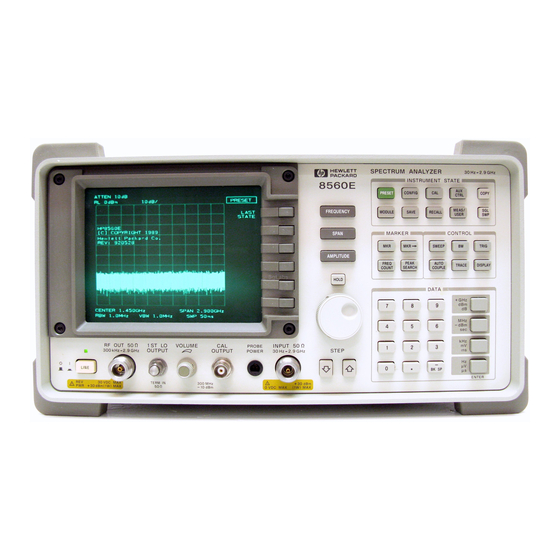
Quick Start Guide Front Panel Overview Front Panel Overview Figure 1-10 Front Panel of an 8560 E-Series or EC- Series Spectrum Analyzer 1. FREQUENCY, SPAN, and AMPLITUDE are the fundamental functions for most measurements. The HOLD key freezes the active function and holds it at the current value until a function key is pressed.
Page 37 300 MHz calibrator signal, a 310.7 MHz IF input, and a ﬁrst LO output. Table 1-2 has a short speciﬁcation summary of these connectors. The IF input is not available with the 8560E/EC, Option 002. A volume knob is provided for making adjustments to the volume of the built-in speaker.
Page 38 −10 dBm to +1 dBm 300 kHz–2.9 GHz (tracking generator output) * Not available with an 8560E/EC Option 002 or Option 327. † Available only with an 8560E/EC Option 002. ‡ LO output of an 8560E/EC Option 002. Chapter 1...
Page 39: Figure 1-11 Display Annotation
Quick Start Guide Front Panel Overview Display Annotation Figure 1-11 Display Annotation 1. Number of video averages. 2. Logarithmic or linear amplitude scale per division. 3. Marker amplitude and frequency. 4. Title area. 5. Data invalid indicator, displayed when analyzer settings are changed before completion of a full sweep.
Page 40 DC coupling selected (The 8563E/EC, 8564E/EC, and 8565E/EC are always dc coupled. AC coupling is available only for an 8560E/EC, 8561E/EC or 8562E/EC spectrum analyzers. The default setting for an 8560E/EC, 8561E/EC or 8562E/EC is ac coupling.) Detector mode set to sample, negative peak, or positive peak...
Page 41: Rear Panel Overview
Quick Start Guide Rear Panel Overview Rear Panel Overview The rear panels of the E-series and EC-series are identical except the earjack on the E-series instruments is located at J1 (see 2, Figure 1-12) while on EC-series instruments, the earjack is located at J7 (see 15, Figure 1-13).
Page 42 Quick Start Guide Rear Panel Overview To prevent damage to the instrument, be sure to set the voltage selector CAUTION to the appropriate value for your local line-voltage output. For more information, refer to the "If You Have A Problem" chapter. 1.
Page 43 For an 8560E/EC, Option 002 (which has a built-in tracking generator), J11 provides an external leveling input. For an Option 005, J11 provides a 0 V to 10 V ramp that corresponds to the sweep ramp that tunes the local oscillator (the same local oscillator sweep ramp that J8 provides).
Page 44: Assistance
Assistance Product maintenance agreements and other customer assistance agreements are available for Agilent Technologies products. For any assistance, contact your nearest Agilent Technologies Sales and Service Ofﬁce. Cleaning The instrument front and rear panels should be cleaned using a soft cloth with water or a mild soap and water mixture.
Page 45: General Safety Considerations
Quick Start Guide General Safety Considerations General Safety Considerations Before this instrument is switched on, make sure it has been WARNING properly grounded through the protective conductor of the ac power cable to a socket outlet provided with protective earth contact.
Page 46: 8560 E-Series And Ec-Series Spectrum Analyzer Documentation Description
8560 E-Series and EC-Series Spectrum Analyzer Documentation Description User's Guide The 8560 E-Series and EC-Series User's Guide applies to the 8560E/EC, 8561E/EC, 8562E/EC, 8563E/EC, 8564E/EC, and 8565E/EC spectrum analyzers. The 8560 E-Series and EC-Series User's Guide includes information about preparing the spectrum analyzer for use, spectrum analyzer functions, common spectrum analyzer measurements, programming fundamentals, and deﬁnitions for remote programming...
Page 47: Manuals Available Separately
How to Order Manuals Each of the manuals listed above can be ordered individually. To order, contact your local Agilent Technologies Sales and Service Ofﬁce. See Table 9-3 on page 681 for a listing of Agilent Technologies sales and service ofﬁces. Chapter 1...
Page 48 Quick Start Guide Manuals Available Separately Chapter 1...
Page 49 Making Measurements...
Page 50: Making Measurements Making Measurements
Making Measurements Making Measurements Making Measurements This chapter demonstrates spectrum analyzer measurement techniques with examples of typical applications. Each application focuses on different features of the Agilent 8560 E-Series and EC-Series spectrum analyzers. The measurement application and procedures covered in this chapter are: •...
Page 51: Example 1: Resolving Closely Spaced Signals (With Resolution Bandwidth)
Spectrum Analyzer Function Used The resolution bandwidth function (RES BW) selects the appropriate IF bandwidth for a measurement. (Agilent Technologies speciﬁes resolution bandwidth as the 3 dB bandwidth of a ﬁlter.) The following guidelines can help you determine the appropriate resolution bandwidth to choose.
Page 52: Figure 2-1 1 Khz Signal Separation
Making Measurements Example 1: Resolving Closely Spaced Signals (with Resolution Bandwidth) To resolve two signals with a frequency separation of 2 kHz, a 1 kHz resolution bandwidth again must be used (see Figure 2-2). Since the spectrum analyzer uses bandwidths in a 1, 3, 10 sequence, the next larger ﬁlter, 3 kHz, would exceed the 2 kHz separation and thus would not resolve the signals.
Page 53 Making Measurements Example 1: Resolving Closely Spaced Signals (with Resolution Bandwidth) Stepping Through a Measurement of Two Signals of Unequal Amplitude This example resolves a third-order intermodulation distortion product with a frequency separation of 700 kHz and an amplitude separation of about 60 dB.
Page 54: Figure 2-3 Bandwidth Shape Factor
Making Measurements Example 1: Resolving Closely Spaced Signals (with Resolution Bandwidth) Figure 2-3 Bandwidth Shape Factor Use a 100 kHz resolution bandwidth ﬁlter to resolve this third-order intermodulation distortion product. The 100 kHz ﬁlter has a typical shape factor of 12:1, a 60 dB bandwidth of 1.2 MHz, and a half-bandwidth value of 600 kHz.
Page 55: Figure 2-4 100 Khz Bandwidth Resolution
Making Measurements Example 1: Resolving Closely Spaced Signals (with Resolution Bandwidth) Figure 2-4 100 kHz Bandwidth Resolution Figure 2-5 300 kHz Bandwidth Resolution Spectrum analyzer sweep time is inversely proportional to the square of NOTE the resolution bandwidth, for bandwidths greater than or equal 300 Hz. So, if the resolution bandwidth is reduced by a factor of ten, the sweep time is increased by a factor of 100.
Page 56: Example 2: Improving Amplitude Measurements With Ampcor
Making Measurements Example 2: Improving Amplitude Measurements with Ampcor Example 2: Improving Amplitude Measurements with Ampcor What Is Ampcor? The amplitude correction function is used to improve the amplitude accuracy of your measurement system. System ﬂatness is often degraded by many things including cable and adapter losses. Additional systematic amplitude errors such as IF gain uncertainty, resolution bandwidth switching uncertainty, and attenuator switching uncertainty can also be corrected.
Page 57: Figure 2-6 Ampcor Measurement Setup
Making Measurements Example 2: Improving Amplitude Measurements with Ampcor Figure 2-6 Ampcor Measurement Setup Set up the measurement. 1. Zero and calibrate the power meter and power sensor. 2. Connect the source output to the power splitter input. Connect the system cable from the spectrum analyzer input to one of the power splitter outputs.
Page 58 Making Measurements Example 2: Improving Amplitude Measurements with Ampcor 6. On the spectrum analyzer, press MORE 1 OF 2 AMPCOR MENU . If there is a correction already loaded, purge it by EDIT AMPCOR pressing . (Or MORE 1 OF 2 DONE EDIT PURGE CORR PURGE DATA...
Page 59 Making Measurements Example 2: Improving Amplitude Measurements with Ampcor Using the ampcor data. 1. With ampcor on, the amplitude measured by the analyzer at the correction-point frequencies should agree with the power meter reading ±0.2 dB. This error is due primarily to the spectrum analyzer marker amplitude resolution, which ranges from 0.017 dB to 0.17 dB, depending upon the log scale selected.
Page 60: Example 3: Modulation
More information about amplitude and frequency modulation can be found in Agilent Technologies Application Note 150-1, literature number 5954-9130. Spectrum Analyzer Functions Used The following procedure describes how to measure signals with AM and FM types of modulation on them.
Page 61: Figure 2-7 An Amplitude-Modulated Signal
Making Measurements Example 3: Modulation Figure 2-7 An Amplitude-Modulated Signal Unequal amplitudes of the lower and upper sidebands indicate NOTE incidental FM on the input signal. Incidental FM can reduce the accuracy of percentage-of-modulation measurements. Figure 2-8 Percentage of Modulation Chapter 2...
Page 62: Figure 2-9 Fm Deviation Test Setup
Making Measurements Example 3: Modulation The following equation also determines percentage of modulation using amplitude units in volts: × ----------------------- - where A = sideband amplitude, in volts = carrier amplitude, in volts Frequency Modulation This section contains general information about frequency modulation, as well as a procedure for calculating FM deviation using a spectrum analyzer.
Page 63: Figure 2-10 Bessel Functions For Determining Modulation Index
Making Measurements Example 3: Modulation 3. Figure 2-10 contains Bessel functions for determining modulation. (Table 2-1 and Table 2-2 on page 63 also contain modulation index numbers for carrier nulls and ﬁrst sideband nulls.) Figure 2-10 Bessel Functions for Determining Modulation Index Table 2-1 Carrier Nulls and Modulation Indexes Order of Carrier Null...
Page 64: Figure 2-11 Markers Show Modulating Frequency
Making Measurements Example 3: Modulation 4. Knowing that the desired deviation is 25 kHz, and choosing the modulation index of the ﬁrst carrier null, calculate the modulating frequency as follows: 25kHz Modulating Frequency --------------- - 2.401 Modulating Frequency 10.412kHz 5. Set the modulation rate on the signal generator to 10.412 kHz. If the signal source doesn't have an accurate internal modulation source, use an external source.
Page 65: Figure 2-12 A Frequency-Modulated Signal
Making Measurements Example 3: Modulation • Gradually change the modulation frequency (or change the amplitude of the modulation signal) and observe the changes in the displayed nulls. Figure 2-12 illustrates a frequency-modulated signal with a small modulation index (modulation index of about 0.2) as it appears on a spectrum analyzer.
Page 66: Figure 2-13 Fm Signal With Carrier At A Null
Making Measurements Example 3: Modulation Figure 2-13 FM Signal with Carrier at a Null Figure 2-14 FM Signal with First Sidebands at a Null NOTE Incidental AM from a source signal can cause the frequency null to shift, resulting in errors to the procedure above.
Page 67: Example 4: Harmonic Distortion
Making Measurements Example 4: Harmonic Distortion Example 4: Harmonic Distortion What Is Harmonic Distortion? Most transmitting devices and signal sources contain harmonics. Measuring the harmonic content of such sources is frequently required. In fact, measuring harmonic distortion is one of the most common uses of a spectrum analyzer.
Page 68: Figure 2-15 Input Signal And Harmonics
Making Measurements Example 4: Harmonic Distortion Figure 2-15 Input Signal and Harmonics 1. Set the video bandwidth to improve visibility by smoothing the noise: a. Press b. Press until MAN is selected. VIDEO BW AUTO MAN ⇓ c. Use the step down key to select the video bandwidth.
Page 69: Figure 2-16 Peak Of Signal Is Positioned At Reference Level For Maximum Accuracy
Making Measurements Example 4: Harmonic Distortion Figure 2-16 Peak of Signal is Positioned at Reference Level for Maximum Accuracy Place a second marker on the second harmonic 1. Set the peak threshold above the noise: a. Press PEAK SEARCH MORE 1 OF 2 PEAK THRESHLD b.
Page 70: Figure 2-17 Harmonic Distortion In Dbc (Marker Threshold Set To −70 Db)
Making Measurements Example 4: Harmonic Distortion Harmonic Distortion in dBc (marker threshold set to −70 dB) Figure 2-17 Find the harmonic distortion (method 1) The difference in amplitude between the fundamental and second harmonic shown in the ﬁgure is about −50 dB, or 0.33 percent harmonic distortion (see Figure 2-18).
Page 71: Figure 2-18 Percentage Of Distortion Versus Harmonic Amplitude
Making Measurements Example 4: Harmonic Distortion Figure 2-18 Percentage of Distortion versus Harmonic Amplitude Find the harmonic distortion (method 2) 1. Another easy way of determining the percent of distortion is to change the units to volts: a. Press . The AMPLITUDE MORE 1 OF 3 AMPTD UNITS...
Page 72 Making Measurements Example 4: Harmonic Distortion An Alternative Harmonic Measurement Method: Procedure B This method is somewhat longer, but because each signal is measured in a narrower span and resolution bandwidth, the signal-to-noise ratio is improved, making the results more accurate. 1.
Page 73: Figure 2-19 Input Signal Displayed In A 1 Mhz Span
Making Measurements Example 4: Harmonic Distortion Figure 2-19 Input Signal Displayed in a 1 MHz Span Measure the second harmonic 1. Press , and the step up key. This MARKER DELTA FREQUENCY › step retunes the spectrum analyzer center frequency to the second harmonic.
Page 74: Figure 2-20 Second Harmonic Displayed In Dbc
Making Measurements Example 4: Harmonic Distortion Figure 2-20 Second Harmonic Displayed in dBc Percent of Harmonic Distortion The total percent of harmonic distortion of a signal is also measured frequently. For this measurement, the amplitude of each harmonic must be measured in linear units (for example, volts) instead of dBc. To display amplitude units in volts, press AMPLITUDE MORE 1 OF 3...
Page 75: Example 5: Third-Order Intermodulation Distortion
Making Measurements Example 5: Third-Order Intermodulation Distortion Example 5: Third-Order Intermodulation Distortion What Is Intermodulation Distortion? In crowded communication systems, signal interference of one device with another is a common problem. For example, two-tone, third-order intermodulation often is a problem in narrow-band systems. When two signals (F and F ) are present in a system, they can mix with the...
Page 76: Figure 2-21 Third-Order Intermodulation Test Setup
Making Measurements Example 5: Third-Order Intermodulation Distortion Figure 2-21 Third-Order Intermodulation Test Setup 2. Set one source to 20 MHz and the other source to 21 MHz, for a frequency separation of 1 MHz. 3. Set the sources equal in amplitude (for this example, we have set the sources to −30 dBm).
Page 77: Figure 2-22 Signals Centered On Spectrum Analyzer Display
Making Measurements Example 5: Third-Order Intermodulation Distortion 8. To resolve the distortion products, reduce the resolution bandwidth until the distortion products are visible: a. Press ⇓ b. Use the step down key to reduce the resolution bandwidth. 9. Reduce the video bandwidth, if necessary. 10.To make sure the input signals are equal in amplitude: a.
Page 78: Figure 2-23 Signal Peak Set To Reference Level
Making Measurements Example 5: Third-Order Intermodulation Distortion MKR → b. Set the reference level to this value by pressing MARKER → REF LVL . Figure 2-23 on page 78 illustrates the resulting display. Figure 2-23 Signal Peak Set to Reference Level Maximize dynamic range 12.Distortion-free dynamic range is important for this type of measurement.
Page 79: Figure 2-24 Intermodulation Distortion Measured In Dbc
Making Measurements Example 5: Third-Order Intermodulation Distortion 13.To measure a distortion product: a. Press to place a marker on a source signal. PEAK SEARCH b. To activate a second marker, press MARKER DELTA c. Press to set the second marker NEXT PK LEFT NEXT PK RIGHT on the peak of the distortion product that is beside the signal...
Page 80: Figure 2-25 Display With Title
Making Measurements Example 5: Third-Order Intermodulation Distortion Figure 2-25 Display with Title Save the measurement information The save and recall functions allow you to store data for later viewing. 15.To save the instrument state: a. Press SAVE SAVE STATE b. Press a softkey to enter the instrument state data into the register (0 to 9) you select.
Page 81: Example 6: Am And Fm Demodulation
Making Measurements Example 6: AM and FM Demodulation Example 6: AM and FM Demodulation What is AM and FM Demodulation? Amplitude modulation (AM) and frequency modulation (FM) are common modulation techniques used to broadcast information. In the United States and Canada, the AM broadcast band is 535 kHz to 1605 kHz, while the FM broadcast band covers 88 MHz to 108 MHz.
Page 82: Figure 2-26 Am And Fm Demodulation Test Setup
Making Measurements Example 6: AM and FM Demodulation Figure 2-26 AM and FM Demodulation Test Setup Set the start and stop frequencies 2. Tune to the FM band by setting the start frequency of the spectrum analyzer to 88 MHz, and the stop frequency to 108 MHz: a.
Page 83: Figure 2-28 . Place A Marker On The Signal Of Interest, Then Demodulate
Making Measurements Example 6: AM and FM Demodulation a. Press to access the demodulation menu. AUX CTRL AM/FM DEMOD b. Activate a marker by pressing MARKER NORMAL c. Position the marker on the signal of interest. If the signal of interest is the highest in amplitude, press directly, PEAK SEARCH...
Page 84: Example 7: Stimulus-Response Measurements
Block Diagram of a Spectrum Analyzer and Tracking Generator System Spectrum Analyzer Functions Used The following procedure describes how to use the 8560E/EC Option 002 spectrum analyzer with built-in tracking generator system to measure the rejection range of a bandpass ﬁlter, which is a type of transmission measurement.
Page 85: Figure 2-30 Transmission Measurement Test Setup
Making Measurements Example 7: Stimulus-Response Measurements The same measurement can be made using an 8560E/EC (without Option 002), Agilent 8561E/EC, Agilent 8562E/EC, Agilent 8563E/EC, Agilent 8564E/EC or Agilent 8565E/EC spectrum analyzer with an Agilent 85640A, Agilent 85644A, or Agilent 85645A tracking generator.
Page 86: Figure 2-31 Tracking-Generator Output Power Activated
If ERR 901 TGFrqLmt appears in the error message area, set the start frequency to 300 kHz. (Stimulus-response measurements using an 8560E/EC Option 002 are speciﬁed from 300 kHz to 2.9 Ghz.) Due to the current resolution of the annotation, changing the start frequency to 300 kHz will be denoted only in smaller spans.
Page 87: Figure 2-32 Adjust Analyzer Settings According To The Measurement Requirement
Making Measurements Example 7: Stimulus-Response Measurements Figure 2-32 Adjust analyzer settings according to the measurement requirement. 6. Decrease the resolution bandwidth to increase sensitivity, and narrow the video bandwidth to smooth the noise. In Figure 2-33, the resolution bandwidth has been decreased to 3 kHz. The minimum resolution bandwidth supported in stimulus-response NOTE measurements is 300 Hz.
Page 88: Figure 2-33 Decrease The Resolution Bandwidth To Improve Sensitivity
Making Measurements Example 7: Stimulus-Response Measurements Figure 2-33 Decrease the resolution bandwidth to improve sensitivity. Tracking Error NOTE Adjusting the resolution bandwidth may result in a decrease in amplitude of the signal. This is known as a tracking error. Tracking errors occur when the tracking generator output frequency does not exactly match the input frequency of the spectrum analyzer.
Page 89: Figure 2-34 Manual Tracking Adjustment Compensates For Tracking Error
Making Measurements Example 7: Stimulus-Response Measurements Figure 2-34 Manual tracking adjustment compensates for tracking error. Calibrate Calibration in a transmission measurement is done using a through (thru). A thru essentially is a conductor that is connected in place of the device under test.
Page 90: Figure 2-35 Guided Calibration Routines Prompt The User
Making Measurements Example 7: Stimulus-Response Measurements Figure 2-35 Guided calibration routines prompt the user. Figure 2-36 The thru trace is displayed in trace B. Normalize Normalization eliminates the frequency response error in the test setup. When normalization is on, trace math is performed on the active trace: A −...
Page 91: Figure 2-37 Normalized Trace
Making Measurements Example 7: Stimulus-Response Measurements The units of the reference level, dB, reﬂect this relative measurement (see Figure 2-37). • To normalize, press until ON is selected. (This NORMLIZE ON OFF softkey is located on the ﬁrst page of the tracking-generator menu.) An arrow appears on each side of the graticule when normalization is activated.
Page 92: Figure 2-38 . Measure The Rejection Range With Delta Markers
Making Measurements Example 7: Stimulus-Response Measurements Figure 2-38 Measure the rejection range with delta markers. Activating normalization changes the softkeys that appear in the amplitude menu: appears, and is replaced by RANGE LVL REF LVL NORM L. Although both these functions reposition the trace on the REF LV display, adjusts attenuation and gain, while...
Page 93: Figure 2-39 Norm Ref Lvl Adjusts The Trace Without Changing Analyzer Settings
Making Measurements Example 7: Stimulus-Response Measurements Figure 2-39 adjusts the trace without changing analyzer NORM REF LVL settings. increases the dynamic range of the measurement by RANGE LVL changing the input attenuator and IF gain. It is equivalent to REF LVL used in signal analysis measurements.
Page 94: Figure 2-40 . Increase The Dynamic Measurement Range By Using Range Lvl
Making Measurements Example 7: Stimulus-Response Measurements Figure 2-40 Increase the dynamic measurement range by using RANGE LVL If the actual measured signal is beyond the gain-compression limit, or below the bottom graticule of the display, an error message will appear in the lower right corner of the display.
Page 95: Figure 2-41 . Normalized Frequency Response Trace Of A Preamplifier
Making Measurements Example 7: Stimulus-Response Measurements Using Range Level versus Using Normalized Reference Level The following example illustrates the difference between RANGE LVL . The normalized frequency response of a NORM REF LVL preampliﬁer is shown in Figure 2-41. The normalized trace is cut off at ⇓...
Page 96: Figure 2-42 Norm Ref Lvl Is A Trace Function
Making Measurements Example 7: Stimulus-Response Measurements Figure 2-42 is a trace function. NORM REF LVL After returning to 0 dB, increase to 30 dB. As NORM REF LVL RANGE LVL shown in Figure 2-43, the trace moves fully within the graticule. Compare the settings: (1) input attenuator value has changed to 40 dB, (2) the marker-amplitude readout displays −6.3 dB, and (3) the ERR 903 A>DLMT error message no longer appears.
Page 97 Making Measurements Example 7: Stimulus-Response Measurements Figure 2-42 shows that is a trace function that can NORM REF LVL position the active trace without changing analyzer settings. The ERR 903 A>DLMT error message is an indicator that the actual measured trace may fall outside of the analyzer measurement range with the current settings.
Page 98: Example 8: External Millimeter Mixers (Unpreselected)
External millimeter mixers can be used to extend the frequency coverage of the 8560 E-Series and EC-Series spectrum analyzers. (The 8560E/EC Option 002 and Option 327 do not have external mixing capability.) Agilent Technologies manufactures external mixers that do not require biasing and cover frequency ranges from 18 GHz to 110 GHz.
Page 99: Figure 2-44 External Mixer Setup (A) Without Bias; (B) With Bias
Making Measurements Example 8: External Millimeter Mixers (Unpreselected) Figure 2-44 External Mixer Setup (a) without Bias; (b) with Bias Good-quality shielded SMA-type cables should be used to connect the NOTE mixer to the spectrum analyzer to ensure that no signal attenuation occurs.
Page 100 Making Measurements Example 8: External Millimeter Mixers (Unpreselected) d. In the external mixer menu, press , then press the FULL BAND step up key until the letter preceding BAND in the active function › area corresponds to the desired frequency band. In this example, we'll look at U-band, which ranges from 40 GHz to 60 GHz, as shown in Figure 2-45.
Page 101: Figure 2-45 Select The Band Of Interest
Making Measurements Example 8: External Millimeter Mixers (Unpreselected) Figure 2-45 Select the band of interest. Save the average conversion-loss value 4. Table lists default conversion-loss values that are stored in the analyzer for each frequency band. These values approximate the values for the Agilent 11970 series mixers.
Page 102: Figure 2-46 Store And Correct For Conversion Loss
Making Measurements Example 8: External Millimeter Mixers (Unpreselected) Figure 2-46 Store and correct for conversion loss. The second method for storing conversion-loss information lets you save individual conversion-loss data points at speciﬁc intervals across the harmonic band, using CNV LOSS VS FREQ To view or enter a conversion-loss data point: a.
Page 103: Figure 2-47 . Signal Responses Produced By A 50 Ghz Signal In U Band
Making Measurements Example 8: External Millimeter Mixers (Unpreselected) Figure 2-47 Signal Responses Produced by a 50 GHz Signal in U Band Identify signals with the frequency-shift method 6. Signal-identiﬁcation routines that identify the signal and images are available on instruments with ﬁrmware revisions ≤920528, or with Option 008.
Page 104: Figure 2-48 Response For Invalid Signals
Making Measurements Example 8: External Millimeter Mixers (Unpreselected) Figure 2-48 Response for Invalid Signals Figure 2-49 Response for Valid Signals Chapter 2...
Page 105: Figure 2-50 Sig Id At Mkr Performed On An Image Signal
Making Measurements Example 8: External Millimeter Mixers (Unpreselected) Identify signals in wide frequency spans identiﬁes signals in wide frequency spans, using SIG ID AT MKR harmonic search. automatically determines the proper SIG ID AT MKR frequency of a signal and displays its value on the spectrum analyzer.
Page 106: Figure 2-51 Sig Id At Mkr Performed On A True Signal
Making Measurements Example 8: External Millimeter Mixers (Unpreselected) Figure 2-51 Performed on a True Signal SIG ID AT MKR Bias The Agilent 11970A Series harmonic mixers mentioned in the previous section do not require bias. Mixers requiring bias can also be used with the 8560 E-Series and EC-Series.
Page 107 Making Measurements Example 8: External Millimeter Mixers (Unpreselected) The open-circuit bias voltage can be as great as +3.5 V through WARNING a source resistance of 300 ohms. Such voltage levels may appear when recalling an instrument state in which an active bias has been stored.
Page 108: Example 9: Adjacent Channel Power Measurement
Making Measurements Example 9: Adjacent Channel Power Measurement Example 9: Adjacent Channel Power Measurement What Is Adjacent Channel Power (ACP)? Adjacent channel power measures the modulation that leaks from the intended channel of a communication device, such as a cellular radio, into an adjacent channel.
Page 109: Figure 2-52 Adjacent Channel Power Measurement Test Setup
Making Measurements Example 9: Adjacent Channel Power Measurement Stepping Through a Basic ACP Measurement In this example, we will be using a transmitter with a carrier frequency of 300 MHz. We will deﬁne the signal that we examine has having a channel bandwidth of 14.0 kHz and a channel spacing requirement of 20.0 kHz, as shown in Figure 2-53.
Page 110: Figure 2-53 Adjacent Channel Power Parameters
Making Measurements Example 9: Adjacent Channel Power Measurement Figure 2-53 Adjacent Channel Power Parameters The ﬁrst step is to set the spectrum analyzer to display the signal under test. 1. Press on the spectrum analyzer to start the measurement PRESET from a deﬁned preset state.
Page 111: Figure 2-54 Adjacent Channel Power Measurement Results
Making Measurements Example 9: Adjacent Channel Power Measurement Access the adjacent channel power (ACP) softkey functions and set up the measurement parameters. 1. Press , then to access the adjacent channel MEAS/USER ACP MENU power menu of softkeys. 2. Press to select the measurement method ACP SETUP METHODS...
Page 112: Figure 2-55 Acp Graph Display
Making Measurements Example 9: Adjacent Channel Power Measurement The adjacent channel power measurement also can be performed with NOTE the spectrum analyzer settings that you choose. For example, if you want to perform the ACP measurement with a speciﬁc resolution bandwidth, or in a particular span, set the spectrum analyzer up in the state that you want, then use performs...
Page 113 Making Measurements Example 9: Adjacent Channel Power Measurement ACP Analog Method Deﬁnition When using the analog method and the ACP auto measurement function for making adjacent channel power measurements, the spectrum analyzer center frequency should be set to the transmitter intended center frequency.
Page 114 Making Measurements Example 9: Adjacent Channel Power Measurement DETECTION: RMS VOLTAGE (POWER DETECTOR) Power detection is invoked during adjacent channel power calculations NOTE but is not available as a detector mode. In addition to the warning message, the instrument-state parameter that is causing the warning will be displayed.
Page 115 Making Measurements Example 9: Adjacent Channel Power Measurement Adjacent Channel Power (ACP) Instrument Setup Settings of the reference level, input attenuation, and display scale are not changed by the ACP auto measurement function. They must be set for optimum dynamic range to optimize accuracy. Although linear and other logarithmic scales are supported, only the log 10 dB per division scale has adequate dynamic range for ACP measurements;...
Page 116 Making Measurements Example 9: Adjacent Channel Power Measurement   ATT N – 3.84dB – -- - DAN L 2M L TODdB   ChBW ChSpacing )log  10dB --------------------- – 20dB – ---------------------------- - ChBW  where: ATTN is the optimum choice of attenuation. ATTN is the attenuator setting chosen within 10 dB increments.
Page 117 Making Measurements Example 9: Adjacent Channel Power Measurement P(x) is the power ratio of the indicated trace data at point x to the reference level. For example, if the trace data is −60 dB, P(x) is 0.000001. SPAN/600 is the spacing of trace data points. NBW is the effective noise bandwidth of the resolution bandwidth used for the measurement.
Page 118 Making Measurements Example 9: Adjacent Channel Power Measurement This correction to x1 through x4 will help the spectrum analyzer results agree with measuring receiver results, because a measuring receiver is speciﬁed to have a −6 dB response at the channel edges. The ACP leakage ratio displayed as MAX ACP is for either the lower or upper adjacent channel, whichever has the higher power.
Page 119 Making Measurements Example 9: Adjacent Channel Power Measurement Set up the spectrum analyzer to display the signal before going to the adjacent channel power softkeys. 1. Press on the spectrum analyzer to start the measurement PRESET from a deﬁned preset state. 2.
Page 120 The following information is applicable as of September 1993. The two-bandwidth method, as described in standard RCR-27B, was not strictly followed by Agilent Technologies in the development of the built-in adjacent channel power functions (ACP). We believe that following the standard exactly as written will not make the intended measurements.
Page 121 The user may want to add +7.25 dB to the (negative) ACP ratios measured, to compensate for the difference between the standard and the Agilent Technologies interpretation of its intent. The 8560 E-Series and EC-Series implementation is consistent with that used in the Agilent 85720A JDC/TDMA Measurement Personality.
Page 122 Making Measurements Example 9: Adjacent Channel Power Measurement is measured with the channel power function, using the wide same trace data as was used by the ACP measurement. That means with the channel power bandwidth set to (2×channel spacing + channel bandwidth), or 792 kHz. The units should be W, mW, or a similar unit.
Page 123: Figure 2-56 . Trigger Configuration For Gated Method, Non-Option 001
Making Measurements Example 9: Adjacent Channel Power Measurement In this implementation , α and the edge of the −∞ dB region are compensated for the effects of a non-zero resolution bandwidth ﬁlter on the effective weighting function. Figure 2-56 Trigger Conﬁguration for Gated Method, Non-Option 001 Chapter 2...
Page 124: Figure 2-57 . Trigger Configuration For Gated Method, Option 001
Making Measurements Example 9: Adjacent Channel Power Measurement Figure 2-57 Trigger Conﬁguration for Gated Method, Option 001 Chapter 2...
Page 125: Example 10: Power Measurement Functions
Making Measurements Example 10: Power Measurement Functions Example 10: Power Measurement Functions What are the Power Measurement Functions? The spectrum analyzer can make several different types of power measurements on complex communication signals. These are in addition to the adjacent channel power measurements discussed in Example 9.
Page 126 Making Measurements Example 10: Power Measurement Functions • The resolution bandwidth may not exceed 100 kHz in the 8560 E-Series and EC-Series spectrum analyzers. A wider resolution bandwidth would cause the video ﬁltering problem mentioned above because the internal video bandwidth in the SAMPLE detection mode is limited by the analyzer hardware to about 450 kHz.
Page 127 Making Measurements Example 10: Power Measurement Functions Making Carrier "Off" Power Measurements Carrier "Off" power measurements are usually made under the same conditions as are the "On" power measurements. Power-indicated accuracy and time-averaged representativeness issues apply here also. RMS detection is usually very important for carrier "Off" measurements because the power tends to be noise-like.
Page 128 Making Measurements Example 10: Power Measurement Functions Stepping through a Carrier Power Measurement A carrier power measurement will be made on a typical cellular radio signal. The signal should be a burst RF signal with about a 20 ms burst period.
Page 129: Example 11: Time-Gated Measurement
Making Measurements Example 11: Time-Gated Measurement Example 11: Time-Gated Measurement What Is Time-Gating? Traditional frequency-domain spectrum analysis provides only limited information for certain signals. Examples of these difﬁcult-to-analyze signal include the following signal types: • Pulsed RF • Time multiplexed •...
Page 130: Figure 2-59 Frequency Of The Combined Signals Of The Radios
Making Measurements Example 11: Time-Gated Measurement Figure 2-59 Frequency of the Combined Signals of the Radios Using the time-gate capability and an external trigger signal, you can see the separate spectrum of radio number one (or radio number 2 if you wish) and identify it as the source of the spurious signal shown as in Figure 2-60 and Figure 2-61.
Page 131: Figure 2-61 . Time-Gated Spectrum Of Signal Number 2
Making Measurements Example 11: Time-Gated Measurement Figure 2-61 Time-Gated Spectrum of Signal Number 2 Time-gating lets you deﬁne a time window, or time gate, during which a measurement will be performed. This permits you to specify the part of a signal that you want to measure, and exclude or mask out other signals that might interfere.
Page 132: Figure 2-62 Block Diagram Of The Spectrum Analyzer With Time Gate
Making Measurements Example 11: Time-Gated Measurement Figure 2-62 Block Diagram of the Spectrum Analyzer with Time Gate The gate within the analyzer is opened and closed based on four factors: • An externally supplied transistor-transistor logic (TTL) signal. • The gate control, or trigger mode (positive or negative edge triggering, or positive or negative level triggering).
Page 133: Figure 2-63 Timing Relationship Of Signals During Gating
Making Measurements Example 11: Time-Gated Measurement Because the pulse trains of signal number 1 and signal number 2 have almost the same carrier frequency, their frequency-domain spectra overlap. Further, the spectrum of pulse train number 2 dominates because signal number 2 has greater amplitude. Without gating, you won't see the spectrum of pulse train number 1;...
Page 134: Figure 2-65 . Using Time-Gating To View Signal 1
Making Measurements Example 11: Time-Gated Measurement Figure 2-65 Using Time-Gating to View Signal 1 Moving the gate so that it is positioned over the middle of pulse train number 2 produces a result such as that shown in Figure 2-67. Here, you see only the spectrum within the pulses of signal number 2;...
Page 135: Figure 2-67 . Using Time-Gating To View Signal 2
Making Measurements Example 11: Time-Gated Measurement Figure 2-67 Using Time-Gating to View Signal 2 Time-gating serves as a useful measurement tool for many different types of signals. However, the signal must be repetitive and have a TTL timing trigger signal available to synchronize the gate. Making Noise Measurements Noise measurements made using a gated measurement technique will vary from the value measured without gating.
Page 136 τ is the time interval over which the peak detection occurs and is equal to the sweeptime/600. Refer to Agilent Technologies Application Note 1303, page 18, for more details. Test Setup and Connection Diagram Figure 2-68 shows a block diagram of the test setup. In Figure 2-68, the signal source is treated as one block.
Page 137: Figure 2-68 Connection Diagram For Time-Gated Spectrum Measurements
Making Measurements Example 11: Time-Gated Measurement Using this measurement setup will allow you to view all signal spectra on the spectrum analyzer and all timing signals on the oscilloscope. The setup will prove to be very helpful when you perform gated measurements on unknown signals.
Page 138 Making Measurements Example 11: Time-Gated Measurement Instrument conﬁgurations for the measurement are: Pulse Generator: Agilent 8112A or equivalent Instrument Connections Pulse period 5 ms (or pulse frequency equal to 200 Hz) Mode norm Pulse width 4 ms High level (HIL) Waveform pulse Low level (LOL)
Page 139 Making Measurements Example 11: Time-Gated Measurement Video bandwidth 3 kHz Gate OFF (Press , then so that OFF is SWEEP GATE ON OFF underlined.) Gate delay 2 ms (Press , use the data keys to enter in GATE DLY [ ] a 2, then press Gate length 1ms (Press...
Page 140: Figure 2-70 Frequency Spectrum Of Signal Without Gating
Making Measurements Example 11: Time-Gated Measurement Figure 2-70 Frequency Spectrum of Signal without Gating To see the effect of time-gating: 1. Press SWEEP 2. Press so that ON is underlined. GATE ON OFF 3. Check the oscilloscope display and ensure that the gate is positioned under the pulse.
Page 141: Figure 2-72 Spectrum Analyzer Display
Making Measurements Example 11: Time-Gated Measurement Figure 2-72 Spectrum Analyzer Display Notice that the gated spectrum is much cleaner than the ungated spectrum. The spectrum you see is the same as would be seen if the signal were on continually. To prove this, turn off the pulse modulation in the signal generator by pressing ;...
Page 142: Figure 2-73 Using Positive Or Negative Triggering
Making Measurements Example 11: Time-Gated Measurement Figure 2-73 Using Positive or Negative Triggering Level Mode In level gate-control mode, an external trigger signal opens and closes the gate directly, without any programmed gate delay or gate length. Either the TTL high level or TTL low level opens the gate, depending on the setting of .
Page 143: Figure 2-74 Time-Domain Parameters
Making Measurements Example 11: Time-Gated Measurement To make a time-gated measurement: 1. Determine how your signal under test appears in the time domain and how it is synchronized to the trigger signal. You need to do this to position the time gate by setting the delay relative to the trigger signal.
Page 144 Making Measurements Example 11: Time-Gated Measurement 2. Set analyzer sweep time greater than 601 times PRI (pulse repetition interval), or longer if MEAS UNCAL appears on the screen. To ensure that the gate is on at least once during each of the 601 digital trace points on the spectrum analyzer, you may need to increase the sweep time of the analyzer.
Page 145: Figure 2-75 Positioning The Gate
Making Measurements Example 11: Time-Gated Measurement Figure 2-75 Positioning the Gate You have ﬂexibility in positioning the gate, but some positions offer a wider choice of resolution bandwidths. A good rule of thumb is to start the gate in the middle of the pulse and have it remain on for one-fourth the pulse duration.
Page 146: Figure 2-77 Setup Time For Interpulse Measurement
Making Measurements Example 11: Time-Gated Measurement You can set the gate length to any value you desire that lets you select the proper portion of the signal of interest to measure. Choosing a narrower gate length forces you to select a wider video bandwidth, as will be discussed in step 5.
Page 147: Figure 2-78 Resolution Bandwidth Filter Charge-Up Effects
Making Measurements Example 11: Time-Gated Measurement Figure 2-78 Resolution Bandwidth Filter Charge-Up Effects Because the resolution-bandwidth ﬁlters are band-limited devices, they require a ﬁnite amount of time to react to changing conditions. Speciﬁcally, the ﬁlters take time to charge fully after the analyzer is exposed to a pulsed signal.
Page 148 Making Measurements Example 11: Time-Gated Measurement Video Bandwidth Just as the resolution-bandwidth ﬁlter needs a ﬁnite amount of time to charge and discharge, so does the video ﬁlter, which is a post-detection ﬁlter used mainly to smooth the measurement trace. Regardless of the length of the real RF pulse, the video ﬁlter sees a pulse no longer than the gate length, and the ﬁlter will spend part of that time charging up.
Page 149 Making Measurements Example 11: Time-Gated Measurement Summary of Time-Gated Measurement Procedure The following is a description of the steps required to perform a time-gated spectrum measurement. 1. Determine how your signal under test appears in the time domain and how it is synchronized to the trigger signal. You need to determine the following: •...
Page 150 Making Measurements Example 11: Time-Gated Measurement "Rules" for Making a Time-Gated Spectrum Measurement This section summarizes the rules described in the previous sections. Table 2-6 Determining Spectrum Analyzer Settings for Viewing a Pulsed RF Signal Spectrum Spectrum Analyzer Setting Comments Analyzer Function Sweep...
Page 151: Figure 2-79 . Gate Positioning Parameters
Making Measurements Example 11: Time-Gated Measurement Figure 2-79 Gate Positioning Parameters Most control settings are determined by two key parameters of the signal under test: the pulse repetition interval (PRI) and the pulse width (τ). If you know these parameters, you can begin by picking some standard settings.
Page 152 Making Measurements Example 11: Time-Gated Measurement Table 2-8 Suggested Sweep Times for a Known Pulse Repetition Interval (PRI) or Pulse Repetition Frequency (PRF) Pulse Repetition Pulse Repetition Sweep Time (minimum) Interval (PRI) Frequency (PRF) ≤50 µs ≥20 kHz 50 ms 100 µs 10 kHz 61 ms...
Page 153 Making Measurements Example 11: Time-Gated Measurement Table 2-9 If You Have a Problem with the Time-Gated Measurement Symptom Possible Cause Suggested Solution Displayed spectrum too low Resolution bandwidth or Widen resolution in amplitude. video bandwidth ﬁlters not bandwidth or video charging fully.
Page 154: Example 12: Making Time-Domain Measurements With Sweep Delay
Making Measurements Example 12: Making Time-Domain Measurements with Sweep Delay Example 12: Making Time-Domain Measurements with Sweep Delay Although spectrum analyzers are primarily frequency-domain devices, they can also show signals in the time domain. The simplest way to do this is to set the SPAN of the analyzer to 0 Hz so that it becomes a ﬁxed-tuned receiver.
Page 155 Making Measurements Example 12: Making Time-Domain Measurements with Sweep Delay Unless the delay sweep function is used, the sweep starts immediately after a valid trigger and lasts as long as the sweep time setting indicates, and the only adjustment that can be made is to increase or decrease the length of the sweep.
Page 156: Figure 2-81 Display Of Zero-Span Without Sweep Delay
Making Measurements Example 12: Making Time-Domain Measurements with Sweep Delay Figure 2-81 Display of Zero-Span without Sweep Delay The sweep delay functions allow you DLY SWP [ ] DLY SWP ON OFF to delay the start of a measurement sweep by up to 65 ms after a trigger signal is received.
Page 157 Making Measurements Example 12: Making Time-Domain Measurements with Sweep Delay The following procedure shows how you can use the sweep delay functions in zero span. 1. Set the center frequency of the spectrum analyzer to the signal of interest. 2. Set the resolution bandwidth and video bandwidth wider than the spectral width of the signal of interest.
Page 158: Example 13: Making Pulsed Rf Measurements
Making Measurements Example 13: Making Pulsed RF Measurements Example 13: Making Pulsed RF Measurements What Is Pulsed RF? A pulsed RF signal is a train of RF pulses with a constant repetition rate, constant pulse width and shape, and constant amplitude. Several procedures for measuring characteristics of a pulsed-RF signal are included in this example.
Page 159: Figure 2-83 Main Lobe And Side Lobes
Making Measurements Example 13: Making Pulsed RF Measurements 6. Increase the sweep time (that is, the sweep becomes slower) until the display ﬁlls in and becomes a solid line (see Figure 2-84). If this line does not ﬁll in, the instrument is not in broadband mode, in which case the following procedures for side lobe ratio, pulse width, and peak pulse power do not apply.
Page 160: Figure 2-84 Trace Displayed As A Solid Line
Making Measurements Example 13: Making Pulsed RF Measurements Figure 2-84 Trace Displayed as a Solid Line Center Frequency, Sidelobe Ratio, and Pulse Width 1. For a pulsed RF signal, the center frequency is at the center of the main lobe (see Figure 2-85). To identify this frequency, simply use the spectrum analyzer peak search function.
Page 161: Figure 2-86 . Markers Show Sidelobe Ratio
Making Measurements Example 13: Making Pulsed RF Measurements 2. To measure the side lobe ratio, with the marker still at the center frequency of the main lobe, press PEAK SEARCH MARKER DELTA . See Figure 2-86. The difference between the amplitude NEXT PEAK of the main lobe and the side lobe is the side lobe ratio.
Page 162: Figure 2-87 Markers Show Pulse Width
Making Measurements Example 13: Making Pulsed RF Measurements Figure 2-87 Markers Show Pulse Width Pulse Repetition Frequency (PRF) Pulse repetition interval (PRI) is the spacing in time between any two adjacent pulse responses, shown in Figure 2-83. Using the function, PRI can easily be inverted to read PRF MARKER 1/DELTA instead.
Page 163: Figure 2-88 . Measuring Pulse Repetition Frequency
Making Measurements Example 13: Making Pulsed RF Measurements Figure 2-88 Measuring Pulse Repetition Frequency Peak Pulse Power and Desensitization Now that you know the main lobe amplitude, the pulse width, and can easily note the spectrum analyzer resolution bandwidth, the peak pulse power can be derived from a relatively simple equation: ) 20log T ) BW...
Page 164 Making Measurements Example 13: Making Pulsed RF Measurements Chapter 2...
Page 165: Softkey Menus
Softkey Menus...
Page 166: Menu Trees
Available only with internal mixing (when set to external mixing, this key is not available). ‡ Not available for an Agilent 8563E/EC, Agilent 8564E/EC, or Agilent 8565E/EC. § Available only when NORMLIZE ON OFF is set to ON. Not available for an Agilent 8560E/EC. Chapter 3...
Page 167: Figure 3-2 Auto Couple Menu Tree
Softkey Menus Menu Trees Figure 3-2 AUTO COUPLE Menu Tree Available only with internal mixing. Chapter 3...
Page 168: Figure 3-3 Aux Ctrl (1 Of 3) Key Menu Tree
AUX CTRL (1 of 3) Key Menu Tree The TRACKING GENRATOR menu shown here is for spectrum analyzers without Option 002 installed. See AUX CTRL menu 3 of 3 for an 8560E/EC with Option 002 installed. INTERNAL MIXER is not shown for an 8560E/EC with Option 002 installed. For an 8560E/EC without Option 002, only the INTERNAL MIXER softkey is available (the softkeys accessed by INTERNAL MIXER are not available).
Page 169: Figure 3-4 Aux Ctrl (2 Of 3) Key Menu Tree
Menu Trees Figure 3-4 AUX CTRL (2 of 3) Key Menu Tree This key is not shown for an 8560E/EC with Option 002 installed and is non-functional for Option 327. † This signal identiﬁcation function is only available with ﬁrmware revisions ≤920528 or with Option 008 installed.
Page 170: Figure 3-5 Aux Ctrl (3 Of 3) Key Menu Tree
Softkey Menus Menu Trees Figure 3-5 AUX CTRL (3 of 3) Key Menu Tree Figure 3-6 BW Key Menu Chapter 3...
Page 171: Figure 3-7 Cal Key Menu Tree
Softkey Menus Menu Trees Figure 3-7 CAL Key Menu Tree Changes to STOP ADJUST if FULL IF ADJ is pressed. † Changes to STORE REF LVL if REF LVL ADJ is pressed. ‡ These functions are only available with ﬁrmware revisions >930809. §...
Page 172: Figure 3-8 Config Key Menu Tree
CONFIG Key Menu Tree Changes to STORE HPIB ADR if pressed. † Not available for an 8560E/EC with Option 002 installed in it and non-functional for instruments with Option 327. Both E-series and EC-series instruments appear as E-series in the instrument ‡...
Page 173: Figure 3-9 Copy Key
Softkey Menus Menu Trees Figure 3-9 COPY Key Figure 3-10 DISPLAY Key Menu Tree Changes to STORE INTENSTY if INTENSTY is pressed. E-series instruments are adjustable. However, EC-series instruments do not require adjustment and are not adjustable. † Changes to STORE FOCUS if FOCUS is pressed. E-Series instruments are adjustable.
Page 174: Figure 3-11 Freq Count Key Menu
Softkey Menus Menu Trees Figure 3-11 FREQ COUNT Key Menu Figure 3-12 FREQUENCY Key Menu Tree MORE 1 OF 2 is displayed under FREQUENCY only on spectrum analyzers with ﬁrmware revision 960401 and later. Figure 3-13 HOLD Key Chapter 3...
Page 175: Figure 3-14 Meas/User Key Menu Tree
Softkey Menus Menu Trees Figure 3-14 MEAS/USER Key Menu Tree Spectrum analyzers with ﬁrmware revisions ≤930809 have fewer power and adjacent channel power (ACP) functions. † See the following ﬁgure for ACP setup menus. ‡ The SPAN softkey is displayed if the markers are not active. §...
Page 176: Figure 3-15 Acp Menu Key Menu Tree
Softkey Menus Menu Trees Figure 3-15 ACP MENU Key Menu Tree The ACP MENU softkey is under the MEAS/USER key. See the preceding ﬁgure. For ﬁrmware revisions ≤930809. † ‡ For ﬁrmware revisions >930809. Figure 3-16 MKR Key Menu Chapter 3...
Page 177: Figure 3-17 Mkr-> Key Menu
Softkey Menus Menu Trees Figure 3-17 MKR-> Key Menu Figure 3-18 MODULE Key Menus MODULE accesses these additional softkeys if the Agilent 85620A mass memory module is attached to the spectrum analyzer. See the Agilent 85620A documentation for more information about these softkeys. †...
Page 178: Figure 3-19 Peak Search Key Menu Tree
Softkey Menus Menu Trees Figure 3-19 PEAK SEARCH Key Menu Tree Changes to if the spectrum analyzer is in MARKER NORMAL zero span or is active. MARKER DELTA Figure 3-20 PRESET Key Chapter 3...
Page 179: Figure 3-21 Recall Key Menu Tree
Softkey Menus Menu Trees Figure 3-21 RECALL Key Menu Tree Available only with internal mixing above 2.9 GHz. † Available with preselected external mixing. Available with internal mixing above 2.9 GHz. Chapter 3...
Page 180: Figure 3-22 Save Key Menu Tree
Softkey Menus Menu Trees Figure 3-22 SAVE Key Menu Tree Available with preselected external mixing. Available with internal mixing above 2.9 GHz. Figure 3-23 SGL SWP Key Figure 3-24 SPAN Key Menu Chapter 3...
Page 181: Figure 3-25 Sweep Key Menu Tree
Softkey Menus Menu Trees Figure 3-25 SWEEP Key Menu Tree This softkey is blanked if GATE CTL EDGE LVL is set to level (LVL). † This softkey becomes LVL POL POS NEG if GATE CTL EDGE LVL is set to level (LVL).
Page 182 Softkey Menus Menu Trees Chapter 3...
Page 183: Key Function Descriptions
Key Function Descriptions...
Page 184: Key Function Tables
Key Function Descriptions Key Function Tables Key Function Tables This chapter describes the functions that are available from the front panel of 8560 E-Series and EC-Series spectrum analyzers. The tables at the start of the chapter list the front-panel keys and softkeys by their functional groups with the location of the key and a very brief description.
Page 185 Key Function Descriptions Key Function Tables Table 4-1 Fundamental Functions Function Keys Access Key Description Selects absolute decibels relative to 1 µV as the dBµV AMPLITUDE amplitude units. Selects absolute decibels relative to 1 mV as the dBmV AMPLITUDE amplitude units. Adds an offset value to displayed frequency values, FREQ OFFSET FREQUENCY...
Page 186 Key Function Descriptions Key Function Tables Table 4-1 Fundamental Functions Function Keys Access Key Description — Activates the frequency span, sets the spectrum analyzer SPAN to center-frequency span mode, and accesses a menu of span related functions. Activates the span width function and sets the spectrum SPAN SPAN analyzer to center-frequency span mode.
Page 187 Key Function Descriptions Key Function Tables Table 4-2 Instrument State Functions Description Instrument State Access Key Keys 3dB POINTS MEAS/USER A peak search is performed, and the 3 dB bandwidth of the largest signal on-screen is displayed in the message area. A peak search is performed, and the 6 dB bandwidth of 6dB POINTS MEAS/USER...
Page 188 Key Function Descriptions Key Function Tables Table 4-2 Instrument State Functions Description Instrument State Access Key Keys AMPCOR MENU Accesses functions that allow you to enter amplitude correction (ampcor) factors to correct system ﬂatness. AMPCOR ON OFF Turns the amplitude correction factors on and off. When this mode is selected, a W appears on the left side of the display.
Page 189 Key Function Descriptions Key Function Tables Table 4-2 Instrument State Functions Description Instrument State Access Key Keys CAL THR AUX CTRL Stores thru calibration in trace B and in instrument state register 9. CARRIER PWR MENU MEAS/USER Accesses carrier power measurement functions. CH EDGES →...
Page 190 Key Function Descriptions Key Function Tables Table 4-2 Instrument State Functions Description Instrument State Access Key Keys DATECODE OPTIONS CONFIG Displays the analyzer ﬁrmware datecode, its instrument serial number, its model number, and any options present. EC-series instruments also appear as Option 007 instruments (Option 007 is the FADC option, which is standard in EC-series instruments).
Page 191 Key Function Descriptions Key Function Tables Table 4-2 Instrument State Functions Description Instrument State Access Key Keys FULL BAND AUX CTRL Selects commonly used frequency bands above 18 GHz and activates the harmonic lock function. FULL IF ADJ Executes a complete adjustment of the IF system for optimum measurement accuracy.
Page 192 Selects negative bias for an external mixer. When this NEGATIVE BIAS AUX CTRL function is selected, a "-" appears on the left side of the display. Not available with an 8560E/EC Option 002. NEW CORR PT Allows you to create a new ampcor correction point. NEXT PEAK...
Page 193 Selects positive mixer bias for an external mixer. When POSITIVE BIAS AUX CTRL this function is selected, a "+" appears on the left side of the display. Not available with an 8560E/EC Option 002. POSTSCLR Displays the value of the post scaler divider within the fractional N assembly.
Page 194 Key Function Descriptions Key Function Tables Table 4-2 Instrument State Functions Description Instrument State Access Key Keys PWR ON STATE SAVE Saves the current state in the power-on register. The spectrum analyzer is set to this state whenever LINE is turned on or when POWER ON is pressed.
Page 195 Key Function Descriptions Key Function Tables Table 4-2 Instrument State Functions Description Instrument State Access Key Keys REF LVL ADJ Permits adjusting the spectrum analyzer internal gain so that when the calibrator signal is connected to the input, the reference level at top screen equals the calibrator amplitude.
Page 196 AUX CTRL Switches the tracking generator output power on and off. A G appears on the left side of the display when this function is active. 8560E/EC Option 002 only. SRC PWR STP SIZE AUX CTRL Sets the step size of the source power level, the source power offset, and the power sweep range function.
Page 197 Key Function Descriptions Key Function Tables Table 4-3 Marker Functions Marker Keys Access Key Description Switches the precision frequency counter COUNTER ON OFF FREQ COUNT ON and OFF (activating a marker if none is present), and displays counter results when the counter is on.
Page 198 Key Function Descriptions Key Function Tables Table 4-3 Marker Functions Marker Keys Access Key Description MKR 1/∆ → CF Sets the center frequency equal to the MKR→ reciprocal of the delta value. For use in zero span mode. MKR 1/∆ → CF STEP Sets the center frequency step size equal to MKR→...
Page 199 Key Function Descriptions Key Function Tables Table 4-4 Control Functions Control Keys Access Key Description Adds the contents of trace A with those of A+B→A TRACE trace B and places the result in trace A. When on, this function continuously A-B→A ON OFF TRACE subtracts the contents of trace B from those...
Page 200 Key Function Descriptions Key Function Tables Table 4-4 Control Functions Control Keys Access Key Description Adjusts the center frequency step size so CF STEP AUTO MAN AUTO COUPLE that when a step key is pressed, the center frequency shifts by the selected step size. Accesses character sets used for creating CHAR SET 1 2 DISPLAY...
Page 201 Key Function Descriptions Key Function Tables Table 4-4 Control Functions Control Keys Access Key Description Sets the trigger to external mode. Connect EXTERNAL TRIG external trigger source to J5 (EXT/GATE TRIG INPUT) on the rear panel. When this mode is selected, a T appears on the left side of the display.
Page 202 Key Function Descriptions Key Function Tables Table 4-4 Control Functions Control Keys Access Key Description Displays and holds the maximum responses MAX HOLD B TRACE of the input signal in trace B. Adjusts the normalized reference position. NORM REF POSN TRACE For use with NORMLIZE ON OFF.
Page 203 Key Function Descriptions Key Function Tables Table 4-4 Control Functions Control Keys Access Key Description Sets the external trigger to trigger on the TRIG POL POS NEG TRIG rising edge (POS) or the falling edge (NEG) of the rear panel trigger input. Accesses a menu of amplitude units.
Page 204: Key Descriptions
J8 output of 0 → 10V. PRESET Front-panel key access: AUX CTRL For 8560E/EC, Agilent 8561E/EC or Agilent .5 V/GHz(FAV) 8563E/EC only. Speciﬁes a 0.5 volts per GHz voltage output at the rear-panel connector J8. Chapter 4...
Page 205 Key Function Descriptions Key Descriptions This is also referred to as the frequency analog voltage (FAV). Connector J8 is labeled LO SWP|FAV OUTPUT, (or LO SWP 0.5 V/GHz on older spectrum analyzers). When using an 8560 E-Series or EC-Series with a tracking generator such as an Agilent 85640A, this softkey must be activated.
Page 206 Key Function Descriptions Key Descriptions When used remotely, the MKBW command ﬁnds the signal bandwidth at 3 dB below the on-screen marker (if a marker is present) or the signal peak (if no on-screen marker is present). Front-panel key access: MEAS/USER When using 6dB POINTS, a peak search is performed 6dBPOINTS...
Page 207 Key Function Descriptions Key Descriptions The trace math function is executed on all subsequent sweeps until it is turned off. An M appears on the left edge of the display to indicate the function is active. The display line is activated as a result of this function; however, it can only be turned off by DSPL LIN ON OFF.
Page 208 Key Function Descriptions Key Descriptions PEAK METHOD The sweep is changed from one sweep, to cover the range of all alternate and adjacent channels, to one sweep for each channel under test. In the faster acceleration, the sweep time is controlled to allow the same number of burst RF cycles in each sweep as would occur in the normal sweep if the spectrum analyzer had 400...
Page 209 Key Function Descriptions Key Descriptions International standards (MKK method) are written around this so the fastest mode has minimal errors due to acceleration. Front-panel key access: MEAS/USER Speeds up the ACP measurement with a minimal ACCELRAT FASTER affect on the accuracy or repeatability. Sweep speeds or measurement techniques are changed to allow faster measurements than those described by the standards.
Page 210: Figure 4-1 Channel Bandwidth Parameters
Key Function Descriptions Key Descriptions ACP AUTO MEASURE turns off the following functions if they are on: • Trace Math • Video Averaging Functions • Frequency Count • Signal Tracking • AM/FM Demodulation The spectrum analyzer center frequency should be set to the transmitter intended center frequency.
Page 211 Key Function Descriptions Key Descriptions Performs an adjacent channel power (ACP) ACP COMPUTE computation on the current trace data without changing the instrument state settings. This computation operates exactly the same as that of ACP AUTO MEASURE, but ACP COMPUTE allows you to control the instrument state settings.
Page 212 Key Function Descriptions Key Descriptions In addition to the warning messages for invalid instrument-state parameters listed above, the following three error messages may be observed in the lower right corner of the display: • ERR 908 BW>>SPCG indicates that the channel bandwidth is too wide, compared to the channel spacing, for a valid computation.
Page 213: Figure 4-2 Acp Graph Display
Key Function Descriptions Key Descriptions The graph can demonstrate how rapidly the ACP ratio changes with channel spacing. The peak method or analog method must be selected since the graph function requires data that is only available with these methods. The upper graticule represents an ACP ratio of 0 dB.
Page 214 Key Function Descriptions Key Descriptions The measurement state parameters that may be changed include: • resolution bandwidth • video bandwidth • span • sweep time • detector mode • gating parameters • trigger parameter • video averaging Front-panel key access: MEAS/USER Executes a routine that adjusts only the current ADJ CURRIF STATE...
Page 215 Key Function Descriptions Key Descriptions The spectrum analyzer chooses appropriate values for these functions depending on the selected frequency and span (or start and stop frequencies). These values are set according to the coupled ratios stored under VBW/RBW RATIO or RBW/SPAN RATIO. If no ratios are stored, default ratios are used instead.
Page 216 Key Function Descriptions Key Descriptions A W appears on the left edge of the display to indicate the function is active. If you have not previously edited or recalled correction data, then the ampcor function is not activated and the message No Correction Loaded appears in the active annunciator area of the display.
Page 217 Key Function Descriptions Key Descriptions Amplitude units are not available in normalized mode. NOTE Makes adjacent channel power (ACP) measurements ANALOG METHOD by measuring continuous power integration versus frequency. Uses an analog method that measures the power in the main and adjacent channels assuming a continuous carrier.
Page 218 Key Function Descriptions Key Descriptions Amplitude correction (ampcor) is on 10 MHz reference is external External mixer bias is greater than 0 mA − External mixer bias is less than 0 mA Front-panel key access: DISPLAY Blanks the annotation from the display (OFF) or ANNOT ON OFF reactivates it (ON).
Page 219 Key Function Descriptions Key Descriptions Front-panel key access: AUTO COUPLE Accesses the softkeys that control auxiliary functions, AUX CTRL for example, the tracking generator and AM or FM demodulation. accesses TRACKING AUX CTRL GENRATOR, INTERNAL MIXER, EXTERNAL MIXER, AM/FM DEMOD, and REAR PANEL. Front-panel key access: AUX CTRL Displays the mean conversion loss for the current...
Page 220 Key Function Descriptions Key Descriptions Front-panel key access: MEAS/USER Selects operation with a monochrome printer, such as an HP ThinkJet, for use by the key. COPY Front-panel key access: CONFIG Subtracts the value of the display line from the B-DL→B contents of trace B and places the result in trace B.
Page 221 Key Function Descriptions Key Descriptions Front-panel key access: MEAS/USER Allows you to enter the period (cycle time) of the burst BURST PERIOD RF signal. The cycle time is needed to set sweep times. Front-panel key access: MEAS/USER Allows you to enter the pulse width ("on" time) of the BURST WIDTH burst RF signal.
Page 222 Key Function Descriptions Key Descriptions The SAVELOCK ON OFF function must be off. If this procedure needs to be interrupted at any time, press ABORT. Front-panel key access: AUX CTRL Activates a procedure to store a thru calibration trace CAL THRU into trace B and into the nonvolatile memory of the spectrum analyzer (for future reference).
Page 223 Key Function Descriptions Key Descriptions Front-panel key access: FREQUENCY Adjusts the center-frequency step-size. When this CF STEP AUTO MAN function is in coupled (AUTO) mode and center frequency is the active function, pressing a step key yields a one-division shift (10 percent of span) in the center frequency for spans greater than 0 Hz.
Page 224 Key Function Descriptions Key Descriptions Moves the center frequency of the spectrum analyzer CHAN UP higher in frequency by one channel spacing. Front-panel key access: MEAS/USER Allows you to set the channel bandwidth for an CHANNEL BANDWDTH adjacent channel power (ACP) measurement. Changing the channel bandwidth will affect the channel power bandwidth setting (CHPWR BW [ ]).
Page 225 Key Function Descriptions Key Descriptions This allows amplitude correction to be entered to compensate for changes in conversion loss with frequency. To enter a new value, use the data keys. To change the displayed frequency, use the step keys. Any changes to the data also affect the mean conversion loss stored under AVERAGE CNV LOSS.
Page 226 Key Function Descriptions Key Descriptions Front-panel key access: CONFIG CONT Sets the measurements, available under the front panel MEASURE key, so that they run continuously. The MEAS/USER selected measurement is repeated unless interrupted by another front panel key. The key does not stop COPY the measurement.
Page 227 Key Function Descriptions Key Descriptions The counted value appears in the upper right corner of the display. Front-panel key access: FREQ COUNT COUNTER Adjusts the resolution of the frequency-count measurement. The resolution ranges from 1 Hz to 1 MHz in decade increments. The default value is 10 kHz.
Page 228: Figure 4-3 Crt Alignment Pattern
Key Function Descriptions Key Descriptions Figure 4-3 CRT Alignment Pattern Chapter 4...
Page 229 E-series instruments in the display when the DATECODE&OPTION key is pressed. EC-series and E-series instruments with Option 007 will both appear as Option 007 instruments. For the 8560E/EC, valid options are: • Option 001 Second IF output •...
Page 230 Key Function Descriptions Key Descriptions For the Agilent 8563E/EC, valid options are: • Option 001 Second IF output • Option 005 Alternate sweep output • Option 007 Fast time domain sweeps (E-series only) • Option 008 Signal Identiﬁcation • Option 026 APC 3.5 front panel RF connector •...
Page 231 Key Function Descriptions Key Descriptions Selects absolute decibels relative to 1 milliwatt as the amplitude units. Front-panel key access: AMPLITUDE Selects absolute decibels relative to 1 µvolt as the dBµV amplitude units. Front-panel key access: AMPLITUDE Selects absolute decibels relative to 1 millivolt as the dBmV amplitude units.
Page 232 Key Function Descriptions Key Descriptions Detector Typical Measurement Mode Positive Good for making sure you do not miss any fast signal Peak peaks. Good for seeing signals that are very close to the noise ﬂoor. Shows a noise ﬂoor that is slightly higher than the actual noise ﬂoor.
Page 233 Key Function Descriptions Key Descriptions DETECTOR Selects the positive-peak detector mode. Used to detect POS PEAK the positive-peak noise level of a trace. This is the detector selected by MAX HOLD. Front-panel key access: TRACE DETECTOR Sets the detector to sample mode. This mode is used SAMPLE with the video averaging and marker noise functions, as well as for the combination of resolution bandwidths...
Page 234 Key Function Descriptions Key Descriptions DSPL LIN Activates a display line that can be adjusted with the ON OFF data keys, the step keys, or the knob. When the display line is ON, pressing DSPL LIN ON OFF again turns the display line OFF.
Page 235 Key Function Descriptions Key Descriptions Data entry is simpliﬁed if you are entering new correction pairs in frequency order. After using the EDIT FREQ softkey and entering the frequency data, a default amplitude is provided and the EDIT AMPL softkey is activated. This default corresponds to the previous amplitude correction value in the list, if one exists, or 0 dB if the new point is the ﬁrst correction on the list.
Page 236 Exits the ampcor menu and returns to the calibration EXIT AMPCOR menu. Front-panel key access: Not available with an 8560E/EC Option 002 and EXT MXR PRE UNPR non-functional in instruments with Option 327. Selects either preselected external mixing mode or unpreselected external mixing mode.
Page 237 (if available), and setting the external mixer bias. Front-panel key access: AUX CTRL No external mixing capabilities are available with an 8560E/EC Option NOTE 002. Resolution bandwidths less than 300 Hz are not available with external mixers.
Page 238 Key Function Descriptions Key Descriptions The FFT results are displayed on the spectrum analyzer in a 10 dB per division logarithmic scale. For the horizontal dimension, the frequency at the left side of the graph is 0 Hz, and at the right side is 300 divided by the sweep time.
Page 239 Key Function Descriptions Key Descriptions Front-panel key access: DISPLAY Displays the fractional N frequency corresponding to FRAC N FREQ the start frequency. This oscillator is used for ﬁne-tuning the local oscillator. Front-panel key access: Sets the trigger to free-run mode. Sweep triggers occur FREE RUN as rapidly as the spectrum analyzer will allow.
Page 240 Key Function Descriptions Key Descriptions Turns off all frequency annotation. This includes the FREQ DSP OFF start and stop frequencies, center frequency, frequency span, marker readouts, center-frequency step size, and signal identiﬁcation to center frequency. Once this key is pressed, there is no way to display the frequency data.
Page 241 Key Descriptions Sets the spectrum analyzer to the center-frequency FULL SPAN span mode and sets the span to the maximum range. Full span is: Spectrum Analyzer Frequency Span 8560E/EC 2.9 GHz Agilent 8561E/EC 6.5 GHz Agilent 8562E/EC 13.2 GHz Agilent 8563E/EC 26.5 GHz...
Page 242 Key Function Descriptions Key Descriptions The gate function requires a gate trigger signal be connected to the rear panel. If the gate is turned on without a signal present, operating other functions like signal tracking, signal identiﬁcation, frequency count, or preselector peaking may cause the spectrum analyzer to stop functioning until it is powered on again.
Page 243 Front-panel key access: AUX CTRL softkey and its lower-level softkeys are not NOTE INTERNAL MIXER available with an 8560E/EC Option 002. However, the INTERNAL MIXER softkey is available with a standard 8560E/EC; its softkey menus are not. Chapter 4...
Page 244 Key Function Descriptions Key Descriptions Sets the spectrum analyzer to the previously selected LAST SPAN span, allowing you to toggle between two settings. For example, you can toggle between zero span and a larger span to view modulation in both the frequency and time domains.
Page 245 Key Function Descriptions Key Descriptions Table 4-6 Mixing Harmonics for Unpreselected External Mixing Frequency Frequency Mixing Conversion Band Range Harmonic Loss (GHz) (Default) 75.0 to 110.0 18− 30 dB 90.0 to 140.0 24− 30 dB 110.0 to 170.0 30− 30 dB 140.0 to 220.0 36−...
Page 246 Key Function Descriptions Key Descriptions Selects the polarity for turning the gate on when LVL POL POS NEG using level triggering for a gated measurement. If (POS) is underlined, the gate will be on while the rear panel trigger input is high. The gate will be on while the trigger input is low if (NEG) is selected.
Page 247: Figure 4-4 Tracking Error
Key Function Descriptions Key Descriptions Figure 4-4 Tracking Error Sets the center frequency equal to the marker MARKER→CF frequency. This function provides a quick way to move a signal to the center of the screen. MKR → Front-panel key access: PEAK SEARCH Sets the center frequency step-size equal to the MARKER→CF STEP...
Page 248 Key Function Descriptions Key Descriptions If a single marker is already on, MARKER DELTA places both an anchor marker and an active (movable) marker at the position of the original, single marker. To move the active marker, use either the knob, the step keys, or the data keys.
Page 249 Key Function Descriptions Key Descriptions Displays and holds the maximum responses of the MAX HOLD B input signal in trace B. In this mode, the trace accepts data from subsequent sweeps and selects the positive-peak detector mode. Front-panel key access: TRACE Available with internal mixing only.
Page 250 Key Function Descriptions Key Descriptions ANALOG METHOD Continuous power integration versus frequency measurement Selects the analog method which measures the power in the main and adjacent channels assuming a continuous carrier. The rms power of that carrier is detected using power detection.
Page 251 Key Function Descriptions Key Descriptions The characteristics of these two types of power change differently with resolution bandwidth changes, so they can be computed algebraically from measurements in two bandwidths. The impulsive powers for all frequencies within each adjacent channel are converted to an equivalent voltage.
Page 252 Key Function Descriptions Key Descriptions The impulsive part of the power is found by the power difference between an ungated measurement and the gated measurement. This method supports TIA/EIA IS-54 NADC-TDMA measurements. Front-panel key access: MEAS/USER Accesses a menu of softkeys: MARKER NORMAL, MARKER DELTA, MARKER 1/DELTA, MKRNOISE ON OFF, SIG TRK ON OFF, and MARKERS OFF.
Page 253 Key Function Descriptions Key Descriptions This function is useful in harmonic distortion measurements, where the delta marker can be used to mark the difference between harmonics, and MKR ∆ -> CF can be used to tune to the frequency of the fundamental.
Page 254 Key Function Descriptions Key Descriptions The MKR∆ → CHPWR BW softkey can be used to change the desired channel power bandwidth to the frequency difference between the two markers that are currently on the signal. The MKR MEAN → CF is then used to center this bandwidth on the display.
Page 255 Key Function Descriptions Key Descriptions Moves you to a new point at the end of the list of NEW CORR PT frequency-amplitude correction points and activates the EDIT FREQ softkey. This is a convenient way to enter a new correction point when you are not currently at the end of the list of corrections.
Page 256 Key Function Descriptions Key Descriptions The normalized reference position may be adjusted between 0.0 and 10.0 (corresponding to the bottom and top graticule lines, respectively) using the data keys, step keys, or knob. The normalized-reference-position adjustment allows measured data to be compared to a reference position, where the difference between the measured data and the reference position represents the gain or loss of the device under test.
Page 257 Key Function Descriptions Key Descriptions To avoid this error, update the CAL THRU or CAL OPN/SHRT state register with the current state before turning NORMLIZE ON OFF on. The CAL THRU state register is state register 9. The CAL OPN/SHRT state register is state register 8.
Page 258: Figure 4-5 . Peak Excursn Defines The Peaks On A Trace
Key Function Descriptions Key Descriptions The excursion values range from 0 dB to 30 dB in log mode, and 0.1 to 10.0 divisions in linear mode. The default value is 6 dB. Any portion of a peak that falls below the peak threshold is also used to satisfy the peak excursion criteria.
Page 259 Selects either the display (DSP) or the graticule PLOT ORG DSP GRAT (GRAT) origin mode. Agilent Technologies plotters allow the user to deﬁne the size of the plot using P1 and P2 parameters. P1 deﬁnes the lower-left corner of the plot, while P2 deﬁnes the upper-right corner.
Page 260 Key Function Descriptions Key Descriptions When DSP is selected, the analyzer scales the full display (excluding the softkey area), so that the corresponding hardcopy plot resides completely within the user-deﬁned P1 and P2 limits. When GRAT is selected, P1 and P2 correspond to the lower-left and upper-right corners of the graticule.
Page 261 Key Function Descriptions Key Descriptions Accesses plotter conﬁguration options to set the PLOTTER CONFIG plotter address, to assign the origin, and to plot trace A, trace B, the graticule, or the frequency annotation. Front-panel key access: CONFIG If the message CONNECT PLOTTER appears brieﬂy in the active function NOTE area of the display when executing any plot function, and there are no other errors, the plotter is not connected to the GPIB.
Page 262 Key Function Descriptions Key Descriptions For internal mixing the marker must be positioned above band 0. Set the trace to clear-write mode, place a marker on the desired point, then press PRESEL AUTO PEAK. The peaking routine zooms to zero span, peaks the preselector tracking, then returns to the original span.
Page 263 Key Function Descriptions Key Descriptions Place a marker on the desired signal on a trace, then press PRESEL MAN ADJ. The current preselector tracking number, which is displayed in the active function block, can be changed using the data keys, the step keys, or the knob.
Page 264 A−B→A A−B+DISPLAY LINE→A ANNOTATION AUTO IF ADJUST BAND LOCK CENTER FREQUENCY 1.45 GHz (8560E/EC) 3.25 GHz (Agilent 8561E/EC) 6.6 GHz (Agilent 8562E/EC) 13.25 GHz (Agilent 8563E/EC) 20 GHz (Agilent 8564E/EC) 25 GHz (Agilent 8565E/EC) CF STEP 290 MHz (8560E/EC) 650 MHz (Agilent 8561E/EC) 1.32 GHz (Agilent...
Page 265 Key Function Descriptions Key Descriptions Table 4-7 Instrument State after Is Executed PRESET Function State FREQUENCY COUNTER FREQUENCY COUNTER 10 kHz RESOLUTION FREQUENCY DISPLAY FREQUENCY MODE CENTER FREQUENCY, SPAN FREQUENCY OFFSET 0 Hz GATE GATE CONTROL EDGE GATE DELAY 3µs GATE LENGTH 1µs GATE POLARITY...
Page 266 Table 4-7 Instrument State after Is Executed PRESET Function State SPAN 2.9 GHz, AUTO (8560E/EC) 6.5 GHz, AUTO (Agilent 8561E/EC) 13.2 GHz, AUTO (Agilent 8562E/EC) 26.5 GHz, AUTO (Agilent 8563E/EC) 40 GHz, AUTO (Agilent 8564E/EC) 50 GHz, AUTO (Agilent 8565E/EC) SQUELCH −120 dBm...
Page 267 RECALL menu. Front-panel key access: SAVE For 8560E/EC Option 002. Activates (ON) or PWR SWP ON OFF deactivates (OFF) the power-sweep function, where the output power of the tracking generator is swept over the power-sweep range chosen. The value of the power-sweep range is displayed in the active function block, when PWR SWP ON OFF is turned on.
Page 268 Key Function Descriptions Key Descriptions Appears only when NORMLIZE ON OFF is set to RANGE LVL ON.Activates the dynamic-range-level function, which corresponds to the top of the display in dBm. RANGE LVL ensures that the displayed range is compression-free by adjusting the input attenuator and IF gain accordingly.
Page 269 Key Function Descriptions Key Descriptions Displays the current coupling ratio between the RBW/SPAN RATIO resolution bandwidth and the frequency span. The ratio is displayed in the active function block, and it is used when resolution bandwidth is in coupled mode. The ratio ranges from 0.002 to 0.10, in a 1, 2, 5 sequence.
Page 270 Key Function Descriptions Key Descriptions Recalls a table of frequency-amplitude correction RECALL AMPCOR points that was previously saved. Front-panel key access: Displays the last error that has occurred. Use the RECALL ERRORS step keys to cycle through accumulated errors. For a list of all error codes and additional error information, refer to Appendix C, "Error Messages", or to the installation and veriﬁcation manual.
Page 271 Key Function Descriptions Key Descriptions The data in this table is sufﬁcient for virtually all applications, because this is the table that allows the spectrum analyzer to meet its published speciﬁcations. 3. User Data Table is the current data table that was saved last and is recalled using the RECALL PRSEL PK softkey.
Page 272 Key Function Descriptions Key Descriptions Displays a menu of eight registers from which trace RECALL TO TR A data can be recalled and placed in trace A. The recall-trace registers appear on two menus: TRACE 0 through TRACE 4 on the ﬁrst page, and TRACE 5 through TRACE 7 on the second page.
Page 273 Key Function Descriptions Key Descriptions When the desired calibration level is reached, STORE REF LVL may be pressed to store the new value in nonvolatile memory. If STORE REF LVL is not pressed, the new value remains in use until a power-on occurs. Front-panel key access: Introduces an offset to all amplitude readouts (for REF LVL OFFSET...
Page 274 Key Function Descriptions Key Descriptions Saves the current table of frequency-amplitude SAVE AMPCOR correction points. Front-panel key access: For use only with internal mixing or preselected SAVE PRSEL PK external mixing. Saves the current preselector-peak data in the user data table. This does not affect the preselector data that is set at the factory or by service personnel.
Page 275 Key Function Descriptions Key Descriptions When is pressed, the preselector data stored by the user does NOTE PRESET not change. However, the factory settings now become active. Factory preselector data always takes precedence over user-activated preselected data, unless the user data is explicitly recalled using RECALL PRSEL PK.
Page 276 Key Function Descriptions Key Descriptions use exactly the same eight save-trace NOTE SAVE TRACE A SAVE TRACE B registers in which to store trace data. Be careful not to overwrite previously saved trace data. Trace-registers 5, 6, and 7 should not be used when using an Agilent 85620A mass memory module.
Page 277 Key Function Descriptions Key Descriptions Activates a 3 line display of the current SCROLL CORR PTS frequency-amplitude correction data. Each correction point consists of a frequency at which the correction should be applied and an amplitude, in dB, of the correction.
Page 278 Key Function Descriptions Key Descriptions For ﬁrmware revisions ≤920528 or for Option 008 only. SIG ID AT MKR Activates a signal-identiﬁcation function that locates the frequency and harmonic number of the mixer response. Place a marker on the desired signal, then activate SIG ID AT MKR.
Page 279 Key Function Descriptions Key Descriptions E Puts the spectrum analyzer in single sweep. SINGLE MEASUR Completes the current measurement and stops further measurements from occurring. If the measurement is already stopped, it is re-started and one measurement is completed. Front-panel key access: MEAS/USER Accesses a menu of softkeys that allow you to SOURCE CAL MENU...
Page 280 AM is inactive. Front-panel key access: AUX CTRL For 8560E/EC Option 002. Allows you to offset the SRC PWR OFFSET displayed power of the tracking generator. Offset values may range from −100 dB to +100 dB.
Page 281 Key Function Descriptions Key Descriptions Front-panel key access: FREQUENCY through Allows you to select which state register to STATE 0 STATE 9 recall or save instrument state information. State registers 8 and 9 are used to store normalization traces. Refer to NOTE tracking-generator calibration softkey descriptions in this chapter for more information.
Page 282 Key Function Descriptions Key Descriptions Activates the sweep time function and accesses a menu SWEEP of sweep-related functions, which are as follows: SWP TIME AUTO MAN, SWEEP CONT SGL, GATE ON OFF, GATED VIDEO, DLY SWP [ ], DLY SWP ON OFF, GATE DLY [ ], GATE LEN [ ], EDGE POL POS NEG, and GATE CTL EDGE LVL.
Page 283 Key Function Descriptions Key Descriptions An E appears in the special functions area at the left side of the display screen when the stimulus response mode is selected. Manual sweep mode only applies to SA mode. If SWP TIME AUTO MAN is set to MAN, the analyzer sweep time coupling defaults to SA mode.
Page 284 Key Function Descriptions Key Descriptions For an 8560E/EC Option 002 see the alternate TRACKING GENRATOR softkey description below. Displays softkey menus only for use with an external tracking generator. The minimum resolution bandwidth that is supported for stimulus-response measurements is 300 Hz.
Page 285 Key Function Descriptions Key Descriptions Accesses a menu of trigger functions: SWEEP CONT TRIG SGL, FREE RUN, VIDEO, LINE, EXTERNAL, and TRIG POL POS NEG. When any mode other than FREE RUN is selected, a T appears in the special functions area at the left side of the display screen.
Page 286 Key Function Descriptions Key Descriptions Turns the video averaging ON or OFF. Video VID AVG ON OFF averaging smooths the displayed trace without using a narrow video bandwidth. The function sets the detector mode to sample mode and smoothes the trace by averaging successive traces with each other.
Page 287 Key Function Descriptions Key Descriptions Sets the display mode for an adjacent channel power VIEW TBL TRCE measurement to show a table (TBL) of the measurement results or to show a representative spectrum trace (TRCE). The trace option is not available when using the burst power measurement method.
Page 288 Key Function Descriptions Key Descriptions WEIGHTNG √ COS OFF Turns on or off the function that does root-raised-cosine weighting of the spectrum data for an ACP measurement. This weighting simulates the ﬁltering expected in the radio receiver to be used. Front-panel key access: MEAS/USER The root-raised-cosine weighting function is described...
Page 289 Programming...
Page 290: Programming Programming Features
Programming Programming Features Programming Features This chapter describes how to operate an 8560 E-Series or EC-Series spectrum analyzer by remote (computer) control. • Setup Procedure for Remote Operation • Communication with the System • Initial Program Considerations • Program Timing •...
Page 291: Setup Procedure For Remote Operation
Programming Setup Procedure for Remote Operation Setup Procedure for Remote Operation The following procedure describes how to connect your equipment for remote operation of the 8560 E-Series or EC-Series spectrum analyzers. Refer to the Chapter 1 for more information on installing, conﬁguring, NOTE and addressing the system.
Page 292: Figure 5-1 8560E Connected To An Hp 9000 Series 300 Computer
Programming Setup Procedure for Remote Operation Figure 5-1 8560E connected to an HP 9000 Series 300 computer. Chapter 5...
Page 293: Communication With The System
Programming Communication with the System Communication with the System This section develops some fundamental techniques for controlling the spectrum analyzer and obtaining reliable measurement results. The spectrum analyzer is remotely controlled with commands that correspond to front-panel softkey functions. It is important to understand how messages are communicated to the spectrum analyzer;...
Page 294: Figure 5-2 Output Statement Example (I)
Programming Communication with the System Figure 5-2 Output Statement Example (I) GPIB An ENTER statement used in conjunction with a spectrum analyzer query returns information to the computer. To return the center-frequency value to the computer, ﬁrst form a query by adding a question mark (?) to the command: Figure 5-3 Output Statement Example (II)
Page 295: Figure 5-4 Output Statement Example (Iii)
Programming Communication with the System Figure 5-4 Output Statement Example (III) GPIB The value of the center frequency above is placed in the variable named "Center." The variable can be printed, stored, or used for other computer functions. Syntax Requirements All of the program examples in this manual show recommended command syntax.
Page 296 Programming Communication with the System Local and Remote Control Whenever the spectrum analyzer is remotely addressed, all front-panel keys and softkeys are disabled, except for the one GPIB related softkey RMT LCL. When the analyzer is remotely addressed, the remote mode (RMT) is selected.
Page 297: Initial Program Considerations
CLEAR is an HP BASIC statement that puts a GPIB instrument (for example, 8560E) in a known state (the preset state) by clearing the input buffer, the output buffer, and the command parser of the speciﬁed instrument so that it is ready for operation. This command can be used to clear devices on the bus singly or in unison.
Page 298: Program Timing
Programming Program Timing Program Timing Most remotely controlled measurements require control of the sweep. The TS (take sweep) command initiates a sweep when the trigger conditions are met. When TS is executed as part of a command sequence, the analyzer starts and completes one full sweep before the next analyzer command is executed.
Page 299: Figure 5-5 Invalid Trace Information
Programming Program Timing Connect the calibrator signal to the analyzer 50Ω INPUT before performing this example. CLEAR 718 OUTPUT 718;"IP;SNGLS;TS;" Initialize analyzer. OUTPUT 718;"CF 300MHZ;SP 1MHZ;" Change measurement range. Figure 5-5 Invalid Trace Information Chapter 5...
Page 300: Figure 5-6 Updated Trace Information
Programming Program Timing The previous program example does not measure with the new analyzer settings as depicted by the data-invalid indicator "*" in the upper right corner. To obtain valid trace information, the trace must be updated with the TS command. Here is the program again, corrected to include the TS command.
Page 301 Programming Program Timing The next example processes trace information with a marker command, MKPK HI (marker peak highest), which selects the highest amplitude level in the trace. Because the program changes the measurement range, the trace information must be updated with TS before MKPK HI is executed.
Page 302: Figure 5-7 Update Trace With Ts Before Executing Marker Commands
Programming Program Timing Figure 5-7 Update trace with TS before executing marker commands. As the example shows, TS is executed after analyzer settings are changed, but before trace information is processed. There are two commands that change the measurement range indirectly: MKCF (marker to center frequency) and MKRL (marker to reference level).
Page 303: Data Transfer To Computer
Programming Data Transfer to Computer Data Transfer to Computer An important part of spectrum-analyzer remote operation is sending and receiving trace data to and from a computer via GPIB. Three requirements apply to all trace data transfers: 1. Determine the trace length. The traces are composed of 601 data points, or trace elements.
Page 304 Programming Data Transfer to Computer Use the TDF (trace data format) command to specify the format before sending data from the spectrum analyzer to the computer. The examples in this section illustrate how to use this command. The examples in this section use the ] (trace A) command. This command transfers data to and from trace A.
Page 305 Programming Data Transfer to Computer The TDF (trace data format) command is used to select measurement or parameter units. Traces are stored internally as integers in the range from 0 to 600, where 0 represents the bottom graticule line and 600 represents the top graticule line.
Page 306 Programming Data Transfer to Computer The left edge of the trace corresponds to the start frequency and the right edge corresponds to the stop frequency. You will need to know start and stop frequencies under which the trace data was measured if you plan to convert from position units to frequency.
Page 307 Programming Data Transfer to Computer Line 10 dimensions array A to 601 elements (one element for each point of trace data). The array is dimensioned using the REAL statement, allowing each array element to accept real-number data. Line 20 sets the analyzer to a desired state. Line 30 calls the subprogram that queries the spectrum analyzer for the required state data.
Page 308 Programming Data Transfer to Computer TDF M (M-format): Return Decimal Numbers in Measurement Units (output only) The measurement units (M) format transfers trace data as ASCII integer values in measurement units, which is the internal format used by the spectrum analyzer. See Figure 5-8 on page 309. The displayed amplitude of each element falls on one of 601 vertical points (with the 601st equal to the reference level).
Page 309: Figure 5-8 Data Transferred In Tdf M Format
Programming Data Transfer to Computer Figure 5-8 Data Transferred in TDF M Format See Table 5-1 on page 304 for an example of how data is sent to the computer using the TDF M format. TDF B (B-Format): Return Binary Numbers in Measurement Units (output only) The binary (B) format transmits data in measurement units, as binary numbers.
Page 310 Programming Data Transfer to Computer Example 6 shows how to transfer data in B-format from the spectrum analyzer to a computer. XAMPLE INTEGER Tra_binary(1:601) ASSIGN @Sa_bin TO 718;FORMAT OFF OUTPUT 718;"IP;CF 300MHZ;SP 20MHZ;SNGLS;TS;" CALL Get_settings(Fa,Fb,Rl,Rb,Vb,St,Lg,Aunits$) OUTPUT 718;"TDF B;TRA?" ENTER @Sa_bin;Tra_binary(*) Line 10 dimensions the array Tra_binary to 601 elements.
Page 311 Programming Data Transfer to Computer Example 7 converts binary values to measurement data and prints them on the computer display. XAMPLE INTEGER Trace_a(1:601) DIM Real_num(1:601) Ref_lvl=0 !0 dBm reference level Log_scale=10 !10dB/division log scale OUTPUT 718;"TDF B;TRA?;" ENTER 718 USING "#,W";Trace_a(*) MAT Real_num= Trace_a FOR X=1 TO 601 Real_num(X)=Ref_level+Log_scale*(Real_num(X)/60-10)
Page 312 Programming Data Transfer to Computer The ﬁrst two characters indicate that the transferred data is in A-block format. "1202" indicates the length of the trace data, expressed in bytes. As previously mentioned, trace data is composed of 601 trace elements. Each trace element is transferred as one word that is composed of two 8-bit bytes.
Page 313 Programming Data Transfer to Computer To send trace data from the computer to the analyzer, refer to Example XAMPLE INTEGER Tra_binary(1:601) DIM Header$[4] OUTPUT 718;"IP;CF 300MHZ;SP 20MHZ;SNGLS;TS;" CALL Get_settings(Fa,Fb,Rl,Rb,Vb,St,Lg,Aunits$) OUTPUT 718;"TDF A;TRA?;" ENTER 718 USING "#,4A,601(W)";Header$,Tra_binary(*) PRINT "PRESS CONTINUE TO RETURN DATA TO THE ANALYZER" PAUSE OUTPUT 718;"IP;TS;VIEW TRA;"...
Page 314 Programming Data Transfer to Computer Example 10 uses the I-block format to separate the # and I characters from the trace data. XAMPLE INTEGER Tra_binary(1:601) DIM Header$[2] OUTPUT 718;"IP;CF 300MHZ;SP 20MHZ;SNGLS;TS;" CALL Get_settings(Fa,Fb,Rl,Rb,Vb,St,Lg,Aunits$) OUTPUT 718;"TDF I;TRA?;" ENTER 718 USING "#,2A,601(W)";Header$,Tra_binary(*) Like the examples for the A-block format, you store format information in a string (Header$) and store the desired trace data in an integer array (Tra_binary).
Page 315 Programming Data Transfer to Computer Transmission Sequence of Data on GPIB Table 5-2 on page 315 shows a GPIB transmission sequence for each format mode. Each one transmits the +10 dBm amplitude level of a one-element trace with the amplitude equal to the reference level. In each case, the HP 9000 Series 200 or 300 computer must be instructed how to interpret the data received correctly.
Page 316: Input And Output Buffers
Programming Input and Output Buffers Input and Output Buffers Features of the 8560 E-Series and EC-Series include the input and output data buffers. This section describes how to take advantage of the buffers and how to avoid potential programming pitfalls. Beneﬁts of an Output Buffer The 64-character input buffer allows you to send several data queries to the spectrum analyzer using only one HP BASIC OUTPUT statement.
Page 317 Programming Input and Output Buffers If you are entering multiple values into multiple variables with one ENTER statement, use a "K" format with the ENTER statement. The spectrum analyzer separates queried values by a line feed with an end-or-identify (EOI) asserted; "K" format recognizes that a new value starts after each line feed with EOI.
Page 318: Figure 5-9 Buffer Summary
Programming Input and Output Buffers If you have a timeout statement in your program, the timeout can occur; this depends on whether the timeout setting is shorter than the pause in the program. Synchronizing Your Program You can use spectrum analyzer queries to synchronize a program. For example, when executing a TS command, if you want to know when the TS command is complete, execute the DONE command immediately after TS.
Page 319: Math Functions
Programming Math Functions Math Functions The analyzer processes and stores measurement results that can be displayed or manipulated arithmetically. This section describes the internal processing of traces and tells how to manipulate data correctly with the math commands. Variables and Traces The analyzer processes all information as variables and trace arrays.
Page 320 Programming Math Functions Adding and Subtracting in dBm Trace-math functions allow easy addition and subtraction of correction values in dBm units. For example, to correct for 3 dB of loss in trace A data values, you can add or subtract trace B, which has been preloaded with +3 dBm or −3 dBm as its data values.
Page 321 Programming Math Functions XAMPLE OUTPUT 718;"IP;SNGLS;CF 300MHZ;SP 20KHZ;RB 10KHZ;RL −10DBM;LG 5DB;TS;" OUTPUT 718;"CLRW TRA; CLRW TRB;TS;" OUTPUT 718;"VIEW TRB;DL −16DBM;" OUTPUT 718;"AMBPL ON;" Line 10 executes an instrument preset, then uses the calibration signal to simulate uncorrected data. The program sets the reference level to −10 dBm, the span to 20 kHz, the center frequency to 300 MHz, the resolution bandwidth to 10 kHz, the log scale to 5 dB, and the sweep to single mode.
Page 322 Programming Math Functions XAMPLE ! PUT TRACES ON SCREEN INTEGER Atrace(1:601) FOR I=1 TO 601 Atrace(I)=300 NEXT I OUTPUT 718;"IP;LG 10DB;SNGLS;TS;" OUTPUT 718 USING "#,K,W,601(W) ,K";"TDF A;TRA#A",1202,Atrace(*),";" OUTPUT 718 USING "#,K,W,601(W) ,K";"TDF A;TRB#A",1202,Atrace(*),";" OUTPUT 718;"AMB ON;" PRINT "PRESS CONTINUE" PAUSE OUTPUT 718;"LN;SNGLS;TS;"...
Page 323: Figure 5-10 Display Units
Programming Math Functions Figure 5-10 Display Units Chapter 5...
Page 324: Creating Screen Titles
Programming Creating Screen Titles Creating Screen Titles Screen titles allow you to label instrument data as shown in Figure 5-11. They can help identify on-screen data or data that you want to store or print. There are commands to create titles remotely and several methods can be used to make titles.
Page 325 Programming Creating Screen Titles No-Format Method This is the simplest method for creating a title. No format is used; you simply enclose the title within string delimiters. A list of delimiters appears below. Refer to Example 1. XAMPLE OUTPUT 718;"TITLE@This is a title@;" In this example, the "@"...
Page 326 Programming Creating Screen Titles Line 30 sends the TITLE command to the analyzer: the #A to specify that the title is in A-block format; the string length; and the contents of the string, which is the actual title. The # sign in the USING statement suppresses any end-of-line characters.
Page 327: Generating Plots And Prints Remotely
(referred to as the P1 and P2 plotter coordinates) deﬁne the lower-left and upper-right corners of the plot. See Figure 5-12 on page 328. These coordinates deﬁne the size of the plot. Table 5-3 on page 328 shows the scaling points for two Agilent Technologies plotters. Chapter 5...
Page 328: Figure 5-12 P1 And P2 Coordinates
Programming Generating Plots and Prints Remotely Figure 5-12 P1 and P2 Coordinates Table 5-3 Scaling Points for Various Plotters Typical Scaling Points Plotting Range Plotter P1x,P1y P2x,P2y X-Axis Y-Axis Agilent 250,279 10250,7479 0 to 10900 0 to 7650 7440 Agilent 250,279 10250,7479 0 to 10900...
Page 329 Programming Generating Plots and Prints Remotely Line 10 queries the plotter for its P1 and P2 coordinates. Line 20 enters the P1 and P2 coordinate values into variables. Line 30 sends the spectrum analyzer PLOT command and the plotter coordinates. Line 40 sends the following statements over the GPIB interface: UNL sets all instruments on the GPIB to unlisten mode;...
Page 330 Programming Generating Plots and Prints Remotely Line 100 returns the spectrum analyzer service requests to their initial condition. Line 110 prints on the computer screen that the plot is done. Plotting Options Perhaps you do not want the entire display contents transferred to the plotter.
Page 331 Programming Generating Plots and Prints Remotely 2. Set the printer to address 1, turn the printer off, and then turn the printer back on. If you cannot locate the address switch on the printer, refer to the printer operation manual. If you want to use a different printer address for remote operation, be sure to modify the examples accordingly.
Page 332: Monitoring System Operation
Programming Monitoring System Operation Monitoring System Operation The programming techniques discussed so far describe communication between the analyzer and the computer, where the sequence of all data transfer is controlled by a computer program. This section describes how the analyzer can interrupt computer operation when the analyzer has attained a particular state.
Page 333 Programming Monitoring System Operation Some of the routines (that are shown above) can be omitted, if only one instrument has been instructed to use the SRQ line, or if a particular instrument has been instructed to use the SRQ line for only one event. Several system-level statements are required to make the computer respond to service requests.
Page 334 Programming Monitoring System Operation The Service-Request Mask The service-request mode is enabled and controlled by the request-service-condition command, RQS. It deﬁnes a service-request mask that speciﬁes which of the status-byte bits can generate a service request. Below, RQS speciﬁes the ERROR-PRESENT and COMMAND-COMPLETE states (bits 5 and 4, respectively) for service requests.
Page 335 Programming Monitoring System Operation In this example, Line 20 indicates that if an interrupt appears (ON INTR 7), the computer is to go to the subroutine Srq (GOSUB Srq). The 7 speciﬁes the interface select code; in this case, it refers to the General Purpose Interface Bus (GPIB).
Page 336 Programming Monitoring System Operation Lines 50 and 60 sends the take-sweep command; during the 10 video averages that will now occur, the computer remains on line 60. When the video averaging is complete, TS is complete and the "command complete" condition is satisﬁed. The computer then branches to the subroutine Srq.
Page 337 Programming Monitoring System Operation See Example 3. XAMPLE OUTPUT 718;"IP;SNGLS;CF 300MHZ;SP 20MHZ;TS;" OUTPUT 718;"VAVG 10;RQS 16;" ON INTR 7 GOSUB Srq ENABLE INTR 7;2 Done=0 OUTPUT 718;"TS;" Idle: IF Done=0 GOTO Idle STOP Srq: Sbyte_1=SPOLL(718) Sbyte_2=SPOLL(705) IF BIT (Sbyte_1,6)=1 THEN PRINT "SERVICE REQUEST",Sbyte_1,"ON ADDRESS 18 "...
Page 338 Programming Monitoring System Operation XAMPLE OUTPUT 718;"IP;SNGLS;CF 300MHZ;SP 20MHZ;TS;" OUTPUT 718;"RQS 16;" ON INTR 7 GOSUB Srq ENABLE INTR 7;2 Done=0 OUTPUT 718;"SRQ 16;" Idle: IF Done=0 GOTO Idle STOP Srq: Sbyte=SPOLL(718) PRINT Sbyte PRINT "INTERRUPT GENERATED" OUTPUT 718;"RQS 0;" Done=1 RETURN Here, on Line 50, a "command complete"...
Page 339: Programming Command Cross Reference
Programming Command Cross Reference...
Page 340: Programming Command Cross Reference Features
Programming Command Cross Reference Programming Command Cross Reference Features Programming Command Cross Reference Features • Front Panel Key Versus Command lists the front panel keys alphabetically and indicates the corresponding programming command, if any. • Programming Command Versus Front Panel Key lists the programming commands by functional groups and indicates the corresponding front panel key.
Page 341: Front Panel Key Versus Command
Programming Command Cross Reference Front Panel Key Versus Command Front Panel Key Versus Command Table 6-1 Front Panel Key Versus Command Programming Command ACPALTCH # ALT CHANNELS ∆MARKER OCC BW DELMKBW SWPOUT 0→10V LO SWP SWPOUT .5 V/GHz (FAV) ACPMETHOD 2BW METHOD MKBW 3dB POINTS...
Page 342 Programming Command Cross Reference Front Panel Key Versus Command Table 6-1 Front Panel Key Versus Command Programming Command DEMOD AM DEMOD ON OFF — AM/FM DEMOD — AMP COR MENU AMPCOR AMP COR ON OFF AMPLITUDE — AMPTD CORRECT AUNITS AMPTD UNITS ACPMETHOD ANALOG METHOD...
Page 343 Programming Command Cross Reference Front Panel Key Versus Command Table 6-1 Front Panel Key Versus Command Programming Command ACPMETHOD BURST PWR METHOD — STOREOPEN, STORESHORT CAL OPN/SHRT STORETHRU CAL THRU — CARRIER PWR MENU CENTER FREQ CF STEP AUTO MAN —...
Page 344 Programming Command Cross Reference Front Panel Key Versus Command Table 6-1 Front Panel Key Versus Command Programming Command MKFCR COUNTER RES COUPLE COUPLING AC DC ADJCRT CRT ADJ PATTERN ID, REV, SER DATECODE & OPTIONS AUNITS dBµV AUNITS dBmV AUNITS AMPCORDATA DELETE CORR PT DEMODT...
Page 345 Programming Command Cross Reference Front Panel Key Versus Command Table 6-1 Front Panel Key Versus Command Programming Command EXTERNAL MXRMODE EXTERNAL MIXER EXTMXR EXT MXR PRE UNPR — FACTORY PRSEL PK FFT MEAS DEMOD FM DEMOD ON OFF — FOCUS FDIAG FRAC N FREQ FREE RUN...
Page 346 Programming Command Cross Reference Front Panel Key Versus Command Table 6-1 Front Panel Key Versus Command Programming Command ADJIF IF ADJ ON OFF — INTENSTY MXRMODE INTERNAL MIXER LAST SPAN RCLS LAST STATE LINE LINEAR HNLOCK LOCK HARMONIC HNLOCK, HNUNLK LOCK ON OFF FDIAG LO FREQ...
Page 347 Programming Command Cross Reference Front Panel Key Versus Command Table 6-1 Front Panel Key Versus Command Programming Command MKR→ MKR ∆→CF MKCF MKR ∆→CF STEP MKSS MKR ∆ →CHPWR BW MKDELCHBW MKR ∆ →SPAN MKSP — MKR 1/∆→CF — MKR 1/∆->CF STEP MKR MEAN →...
Page 348 Programming Command Cross Reference Front Panel Key Versus Command Table 6-1 Front Panel Key Versus Command Programming Command PLOTSRC PLOT ANNOT PLOTSRC PLOT GRATICUL PLOTORG PLOT ORG DSP GRAT PLOTSRC PLOT TRACE A PLOTSRC PLOT TRACE B — PLOTTER ADDRESS PLOTSRC PLOTTER CONFIG MBIAS...
Page 349 Programming Command Cross Reference Front Panel Key Versus Command Table 6-1 Front Panel Key Versus Command Programming Command RECALL ERRORS RCLOSCAL RECALL OPN/SHRT — RECALL PRSEL PK RCLS RECALL STATE RCLTHRU RECALL THRU RCLT RECALL TO TR A RCLT RECALL TO TR B REF LVL RLCAL REF LVL ADJ...
Page 350 Programming Command Cross Reference Front Panel Key Versus Command Table 6-1 Front Panel Key Versus Command Programming Command MKTRACK SIG TRK ON OFF MEAS SINGLE MEASURE — SOURCE CAL MENU — SPACE — SPACING/BANDWDTH SPAN — SPAN ZOOM SQUELCH SQUELCH ON OFF SRCPOFS SRC PWR OFFSET SRCPWR...
Page 351 Programming Command Cross Reference Front Panel Key Versus Command Table 6-1 Front Panel Key Versus Command Programming Command VBW/RBW RATIO SWPOUT V/GHz .25 .50 VAVG VID AVG ON OFF TM, VTL VIDEO VIDEO BW AUTO MAN VIEW VIEW A VIEW VIEW B ACPRSLTS VIEW TBL TRCE...
Page 352: Programming Command Versus Front Panel Key
Programming Command Cross Reference Programming Command Versus Front Panel Key Programming Command Versus Front Panel This table is a functional sort of the programming commands. Alternate commands common to the 8560 E-Series and EC-Series, and the Agilent 8566 and Agilent 8568, are shown within parentheses. For further information about alternate commands, see "Agilent 8566A and Agilent 8568A Compatible Commands"...
Page 353 Programming Command Cross Reference Programming Command Versus Front Panel Key Table 6-2 Programming Command Functional Index Function Command Corresponding Key Description Category Function SS AUTO CF STEP AUTO MAN Auto-couples center-frequency (AUTO) step-size (CS). ST AUTO SWP TIME AUTO MAN Auto-couples sweep time (CT).
Page 354 Programming Command Cross Reference Programming Command Versus Front Panel Key Table 6-2 Programming Command Functional Index Function Command Corresponding Key Description Category Function AUXILIARY PSDAC PRESEL MAN ADJ Adjusts or returns CONTROL preselector-peak DAC number. (continued) RCLOSCAL RECALL OPN/SHRT Recalls stored open/short trace calibration data.
Page 355 Programming Command Cross Reference Programming Command Versus Front Panel Key Table 6-2 Programming Command Functional Index Function Command Corresponding Key Description Category Function CALIBRA TION ADJALL REALIGN LO &IF Initiates power-on adjustment sequence. ADJCRT CRT ADJ PATTERN Initiates CRT adjustment patterns.
Page 356 Programming Command Cross Reference Programming Command Versus Front Panel Key Table 6-2 Programming Command Functional Index Function Command Corresponding Key Description Category Function DISPLAY ANNOT ANNOT ON OFF Turns annotation on or off. BLANK BLANK A BLANK B Stores and blanks speciﬁed trace register (A4 and B4).
Page 357 Programming Command Cross Reference Programming Command Versus Front Panel Key Table 6-2 Programming Command Functional Index Function Command Corresponding Key Description Category Function PSDAC PRESEL MAN ADJ Adjusts or returns preselector-peak DAC number. DATECODE &OPTIONS Returns analyzer ﬁrmware revision date. RLCAL REF LVL ADJ Calibrates reference level.
Page 358 Programming Command Cross Reference Programming Command Versus Front Panel Key Table 6-2 Programming Command Functional Index Function Command Corresponding Key Description Category Function ACPBRPER BURST PERIOD Sets the burst period for an adjacent channel power measurement. ACPBRWID BURST WIDTH Sets the burst width for an adjacent channel power measurement.
Page 359 Programming Command Cross Reference Programming Command Versus Front Panel Key Table 6-2 Programming Command Functional Index Function Command Corresponding Key Description Category Function MEASURE/ CHPWRBW CHPWR BW [ ] Sets the bandwidth for the desired channel power. USER ∆MARKER OCC BW (continued) DELMKBW Measures the occupied power...
Page 360 Programming Command Cross Reference Programming Command Versus Front Panel Key Table 6-2 Programming Command Functional Index Function Command Corresponding Key Description Category Function PSTATE SAVELOCK ON OFF Protects saved states (save lock). RCLS RECALL STATE Recalls previously saved state (RC). RCLT RECALL TO TRA Recalls speciﬁed trace data.
Page 361 Programming Command Cross Reference Programming Command Versus Front Panel Key Table 6-2 Programming Command Functional Index Function Command Corresponding Key Description Category Function TRACE DETECTOR MODES Speciﬁes video detector type. A − B into A (C1 and C2). TRACE MATH A−B→A ON OFF A −...
Page 362 Programming Command Cross Reference Programming Command Versus Front Panel Key Agilent 8566A and Agilent 8568A Compatible Commands This is a list of commands from the Agilent 8566A and Agilent 8568A spectrum analyzers that use the same mnemonic as the 8560 E- Series and EC-Series.
Page 363 Programming Command Cross Reference Programming Command Versus Front Panel Key Table 6-3 Backward-Compatible Commands Agilent Preferred Agilent 8560 Description 8566A E-Series and EC-Series Agilent Command 8568A Command MKPK HI Marker to highest peak MKCF Marker to Center Frequency MKSS Marker Frequency to Center Frequency Step Size MKRL Marker to Reference Level...
Page 364 Programming Command Cross Reference Programming Command Versus Front Panel Key Table 6-3 Backward-Compatible Commands Agilent Preferred Agilent 8560 Description 8566A E-Series and EC-Series Agilent Command 8568A Command TRB? Trace B Data Chapter 6...
Page 365 Programming Command Cross Reference Programming Command Versus Front Panel Key Mass Memory Module Commands The following commands are available when the Agilent 85620A mass memory module is being used with the spectrum analyzer. See the documentation for the Agilent 85620A for more information. Table 6-4 Mass Memory Module Commands ABORT...
Page 366 Programming Command Cross Reference Programming Command Versus Front Panel Key Table 6-4 Mass Memory Module Commands IF THEN ELSE ENDIF forms a decision and branching construct. Places the greatest integer that is less than or equal to the source value into the destination. KEYCLR Clears softkeys 1 through 6.
Page 367 Programming Command Cross Reference Programming Command Versus Front Panel Key Table 6-4 Mass Memory Module Commands Sets the origin. OUTPUT Allows the spectrum analyzer to send data to other devices on the GPIB. Moves the pen to a vector location on the spectrum analyzer screen relative to the reference coordinates (0,0).
Page 368 Programming Command Cross Reference Programming Command Versus Front Panel Key Table 6-4 Mass Memory Module Commands Returns the sum of the amplitudes of the trace elements in measurement units. SUMSQR Returns the sum of the squares of the amplitude of each trace element.
Page 369: Language Reference
Language Reference...
Page 370: Language Reference Features
Language Reference Language Reference Features Language Reference Features This chapter contains complete information for the programming commands available to operate an 8560 E-Series or EC-Series spectrum analyzer. Cross-reference information for the softkeys and programming commands are supplied in Chapter 6. The commands available when using the mass memory module with the spectrum analyzer are listed in Table 6-4 on page 365.
Page 371: Syntax Diagram Conventions
Language Reference Syntax Diagram Conventions Syntax Diagram Conventions Command syntax is represented pictorially. Figure 7-1 Command Syntax Figure • Ovals enclose command mnemonics. The command mnemonic must be entered exactly as shown. • Circles and ovals surround secondary keywords or special numbers and characters.
Page 372: Figure 7-2 Numeric Value Query Response
Language Reference Syntax Diagram Conventions Query Responses Figure 7-2 Numeric Value Query Response Commands that set a function to a numeric value can be queried to determine the current setting of that function. For example, the CF command sets the center frequency to a numeric value in hertz. The format for the response to a CF query command is shown above.
Page 373 Language Reference Syntax Diagram Conventions Table 7-1 Syntax Elements Syntax Deﬁnition/Range Component delimiter ! $ % & ' / : = \ @ &^ ` | ~ A character, chosen from the above list, marks the beginning and end of a string of characters. For simpliﬁed use, choose delimiters that are not the same as any character within the string they delimit.
Page 374 Language Reference Syntax Diagram Conventions In the syntax diagrams, characters and secondary keywords are shown within circles or ovals. Characters and secondary keywords must be entered exactly as shown. Table 7-2 Characters and Secondary Keywords (Reserved Words) Element Description ampere (unit); A-block data format; external mixer frequency band alternating current (coupling) all (marker off, plot screen) amplitude modulation (DEMOD)
Page 375 Language Reference Syntax Diagram Conventions Table 7-2 Characters and Secondary Keywords (Reserved Words) Element Description internal (reference, mixer mode) external mixer frequency band external mixer frequency band kilohertz (unit) kilohertz (unit) LAST previous state before a change or previous span before a change LEVEL trigger level LINE...
Page 376 Language Reference Syntax Diagram Conventions Table 7-2 Characters and Secondary Keywords (Reserved Words) Element Description stimulus response (sweep time coupling) trace A trace B external mixer frequency band microamp (unit) UNIFORM FFT window format UNPR unpreselected external mixer mode increment the parameter microvolt (unit) microsecond (unit) volt (unit);...
Page 377: Programming Commands
Language Reference Programming Commands Programming Commands This chapter contains the programming commands. Each spectrum analyzer command is described in this section. Before using this part of the manual, you may want to refer to Chapter 5 of this manual. Chapter 7...
Page 378: Acpaccl Accelerate Adjacent Channel Power Measurement
Language Reference ACPACCL Accelerate Adjacent Channel Power Measurement ACPACCL Accelerate Adjacent Channel Power Measurement Syntax Figure 7-4 ACPACCL Syntax Description The ACPACCL command sets the acceleration of the adjacent channel power measurement to normal (NRM), faster (FASTR), or fastest (FASTS). The ACP measurement techniques are changed when faster and fastest are selected to speed up the measurement process.
Page 379: Figure 7-5 Acpaccl Query Response
Language Reference ACPACCL Accelerate Adjacent Channel Power Measurement Query Response Figure 7-5 ACPACCL Query Response Example OUTPUT 718;"ACPACCL FASTR;" Chapter 7...
Page 380: Acpalpha Adjacent Channel Power Alpha Weighting
Language Reference ACPALPHA Adjacent Channel Power Alpha Weighting ACPALPHA Adjacent Channel Power Alpha Weighting Syntax Figure 7-6 ACPALPHA Syntax Description The ACPALPHA command is used to set the alpha weighting for an adjacent channel power measurement. Parameters number unitless real number between 0 and 1 Query Response Figure 7-7 ACPALPHA Query Response...
Page 381: Acpaltch Adjacent Channel Power Alternate Channels
Language Reference ACPALTCH Adjacent Channel Power Alternate Channels ACPALTCH Adjacent Channel Power Alternate Channels Syntax Figure 7-8 ACPALTCH Syntax Description The ACPALTCH command sets the number of alternate channels to be measured by an adjacent channel power measurement to either 0, 1, or 2.
Page 382: Acpbrper Adjacent Channel Power Burst Period
Language Reference ACPBRPER Adjacent Channel Power Burst Period ACPBRPER Adjacent Channel Power Burst Period Syntax Figure 7-10 ACPBRPER Syntax Description The ACPBRPER command sets the cycle time (period) of the burst RF signal. The cycle time is needed to set the sweep times when using the peak, two bandwidth, burst power, and gated methods for adjacent channel power measurements.
Page 383: Acpbrwid Adjacent Channel Power Burst Width
Language Reference ACPBRWID Adjacent Channel Power Burst Width ACPBRWID Adjacent Channel Power Burst Width Syntax Figure 7-12 ACPBRWID Syntax Description The ACPBRWID command sets the on-time (pulse width) of the burst RF signal. The pulse width is needed to set the gating times when using the gated method for adjacent channel power measurements.
Page 384: Acpbw Adjacent Channel Power Channel Bandwidth
Language Reference ACPBW Adjacent Channel Power Channel Bandwidth ACPBW Adjacent Channel Power Channel Bandwidth Syntax Figure 7-14 ACPBW Syntax Description The ACPBW command sets the bandwidth of the channels as an active function for the ACPMEAS and ACPCOMPUTE commands. The channel bandwidth cannot be greater than the channel spacing.
Page 385: Acpcompute Adjacent Channel Power Compute
Language Reference ACPCOMPUTE Adjacent Channel Power Compute ACPCOMPUTE Adjacent Channel Power Compute Syntax Figure 7-16 ACPCOMPUTE Syntax Description The ACPCOMPUTE command calculates the adjacent channel power (ACP) of a transmitter based on the data that is on the display. This function does not make a new measurement before computing.
Page 386 Language Reference ACPCOMPUTE Adjacent Channel Power Compute to obtain a valid measurement. • ERR 910 SPAN>ACP indicates that the frequency span is too wide, compared to the channel bandwidth, to obtain an accurate measurement. If any of these errors occurs, the measurement is not completed. To make a measurement, adjust your instrument state settings depending on the error that has occurred.
Page 387: Acpfrqwt Adjacent Channel Power Frequency Weighting
Language Reference ACPFRQWT Adjacent Channel Power Frequency Weighting ACPFRQWT Adjacent Channel Power Frequency Weighting Syntax Figure 7-17 ACPFRQWT Syntax Description The ACPFRQWT command can be used to effect the frequency weighting when making an adjacent channel power measurement. Weighting is not used in the measurement if OFF has been selected. Root-raised-cosine weighting is selected with the RRCOS parameter.
Page 388: Acpgraph Adjacent Channel Power Graph
Language Reference ACPGRAPH Adjacent Channel Power Graph ACPGRAPH Adjacent Channel Power Graph Syntax Figure 7-19 ACPGRAPH Syntax Description The ACPGRAPH command turns on or off a graphical representation of the adjacent channel power ratio, for the selected channel bandwidth, as a function of the channel spacing. The command requires data that is only available with the peak or analog method.
Page 389: Figure 7-20 Acpgraph Query Response
Language Reference ACPGRAPH Adjacent Channel Power Graph Query Response Figure 7-20 ACPGRAPH Query Response Example OUTPUT 718;"ACPGRAPH ON;" Chapter 7...
Page 390: Acplower Lower Adjacent Channel Power
Language Reference ACPLOWER Lower Adjacent Channel Power ACPLOWER Lower Adjacent Channel Power Syntax Figure 7-21 ACPLOWER Syntax Description The ACPLOWER query command returns the power ratio result of the adjacent channel power measurement for the lower frequency channel. Query Response Figure 7-22 ACPLOWER Query Response Example...
Page 391: Acpmax Maximum Adjacent Channel Power
Language Reference ACPMAX Maximum Adjacent Channel Power ACPMAX Maximum Adjacent Channel Power Syntax Figure 7-23 ACPMAX Syntax Description The ACPMAX query command returns the maximum adjacent channel power of the adjacent channel power measurement. Query Response Figure 7-24 ACPMAX Query Response Example REAL Max_chpwr OUTPUT 718;"ACPMAX?;"...
Page 392: Acpmeas Measure Adjacent Channel Power
Language Reference ACPMEAS Measure Adjacent Channel Power ACPMEAS Measure Adjacent Channel Power Syntax Figure 7-25 ACPMEAS Syntax Description The ACPMEAS command makes a measurement and calculates the adjacent channel power (ACP) of a transmitter. The measurement determines the leakage power that is in the adjacent channels from the carrier.
Page 393 Language Reference ACPMEAS Measure Adjacent Channel Power The current channel spacing and channel bandwidth values are also displayed as follows: • channel spacing (ACPSP) • channel bandwidth (ACPBW) Example REAL Lower,Upper,Total_pwr,Max_acp OUTPUT 718;"ACPMEAS;" OUTPUT 718;"ACPLOWER?;" ENTER 718;Lower OUTPUT 718;"ACPUPPER?;" ENTER 718;Upper OUTPUT 718;"ACPPWRTX?;"...
Page 394: Acpmethod Adjacent Channel Power Measurement Method
Language Reference ACPMETHOD Adjacent Channel Power Measurement Method ACPMETHOD Adjacent Channel Power Measurement Method Syntax Figure 7-26 ACPMETHOD Syntax Description The ACPMETHOD command is used to select the measurement method for making an adjacent channel power measurement (ACP). The selections include the analog method, peak method, two bandwidth method, burst method and gated method.
Page 395 Language Reference ACPMETHOD Adjacent Channel Power Measurement Method There are 600 measurement cells per sweep, so this sets one burst RF cycle per measurement cell. This method supports 1993 MKK standard for PDC systems and the 1993 RCR standards for PHP systems. 2BW METHOD Two bandwidth, transient and random peak measurement for TDMA This method is meant for use with burst signals.
Page 396: Figure 7-27 Acpmethod Query Response
Language Reference ACPMETHOD Adjacent Channel Power Measurement Method The impulsive part of the power is found by the power difference between an ungated measurement and the gated measurement. This method supports the TIA/EIA IS-54 NADC/TDMA measurements. Parameters ANALOG, PEAK, TWOBW, BURST, GATED Preset State Analog Query Response...
Page 397: Acpmstate Adjacent Channel Power Measurement State
Language Reference ACPMSTATE Adjacent Channel Power Measurement State ACPMSTATE Adjacent Channel Power Measurement State Syntax Figure 7-28 ACPMSTATE Syntax Description The ACPMSTATE command sets the parameters of the measurement state to either the default state (determined by the rest of the setup) or the current state.
Page 398: Figure 7-29 Acpmstate Query Response
Language Reference ACPMSTATE Adjacent Channel Power Measurement State Parameters CURR (current), DFLT (default) Query Response Figure 7-29 ACPMSTATE Query Response Example OUTPUT 718;"ACPMSTATE CURR;" Chapter 7...
Page 399: Acppwrtx Total Power Transmitted
Language Reference ACPPWRTX Total Power Transmitted ACPPWRTX Total Power Transmitted Syntax Figure 7-30 ACPPWRTX Syntax Description The ACPPWRTX query command returns the result of the total power transmitted calculation of the adjacent channel power measurement. The measurement must be made with the analog or burst power method selected.
Page 400: Acprslts Adjacent Channel Power Measurement Results
Language Reference ACPRSLTS Adjacent Channel Power Measurement Results ACPRSLTS Adjacent Channel Power Measurement Results Syntax Figure 7-32 ACPRSLTS Syntax Description The ACPRSLTS command returns an array of power data resulting from an adjacent channel power measurement of an RF signal. The size of the array is determined by the number of alternate channel pairs selected by the ACPALTCH command.
Page 401 Language Reference ACPRSLTS Adjacent Channel Power Measurement Results The measurement method and the number of alternate channels you have selected determine the size of the data array that will be returned by the ACPRSLTS command. Table 7-1 indicates the values that will be returned for each method.
Page 402: Figure 7-33 Acprslts Query Response
Language Reference ACPRSLTS Adjacent Channel Power Measurement Results Table 7-4 Alternate Channels Alternate Channels Used For Calculation Number of Values Returned Channels main channel 1 set lower adjacent channel (see Table 7-1 on page 372) upper adjacent channel above channels plus: 2 sets ﬁrst alternate lower channel (see Table 7-1 on page 372)
Page 403: Acpsp Adjacent Channel Power Channel Spacing
Language Reference ACPSP Adjacent Channel Power Channel Spacing ACPSP Adjacent Channel Power Channel Spacing Syntax Figure 7-34 ACPSP Syntax Description The ACPSP command sets channel spacing as the active function for the ACPMEAS and ACPCOMPUTE commands. The spacing is set between a minimum of 100 Hz to a maximum of 50 GHz.
Page 404: Figure 7-35 Acpsp Query Response
Language Reference ACPSP Adjacent Channel Power Channel Spacing Query Response Figure 7-35 ACPSP Query Response Example REAL Channelsp Channelsp = 12.5E3 OUTPUT 718;"ACPSP ";Channelsp;"HZ;" Chapter 7...
Page 405: Acpt Adjacent Channel Power T Weighting
Language Reference ACPT Adjacent Channel Power T Weighting ACPT Adjacent Channel Power T Weighting Syntax Figure 7-36 ACPT Syntax Description The ACPT command is used to set the T used in weighting for an adjacent channel power measurement. Parameters real number between 1 µs and 1 s number Query Response Figure 7-37...
Page 406: Acpupper Upper Adjacent Channel Power
Language Reference ACPUPPER Upper Adjacent Channel Power ACPUPPER Upper Adjacent Channel Power Syntax Figure 7-38 ACPUPPER Syntax Description The ACPUPPER query command returns the power ratio result of the adjacent channel power measurement for the upper frequency channel. Query Response Figure 7-39 ACPUPPER Query Response Example...
Page 407: Adjall Lo And If Adjustments
Language Reference ADJALL LO and IF Adjustments ADJALL LO and IF Adjustments Syntax Figure 7-40 ADJALL Syntax Description The ADJALL command activates the RF local oscillator (LO) and intermediate frequency (IF) alignment routines. These are the same routines that occur when the spectrum analyzer is switched on. Commands following ADJALL are not executed until after the analyzer has ﬁnished the alignment routines.
Page 408: Adjcrt Adjust Crt Alignment
Language Reference ADJCRT Adjust CRT Alignment ADJCRT Adjust CRT Alignment Syntax Figure 7-41 ADJCRT Syntax Description The ADJCRT command activates a CRT adjustment pattern, shown in Figure 7-42 on page 409. Use the X POSN, Y POSN, and TRACE ALIGN adjustments, available from the rear panel on E-series instruments, to align the display.
Page 409: Figure 7-42 Crt Alignment Pattern
Language Reference ADJCRT Adjust CRT Alignment Figure 7-42 CRT Alignment Pattern Example OUTPUT 718;"ADJCRT;" OUTPUT 2;CHR$(255)&"K"; PRINT TABXY(0,1);"USE X POSN AND Y POSN" PRINT TABXY(0,3);"TO ADJUST THE DISPLAY" INPUT "THEN PRESS ENTER",Ans$ OUTPUT 718;"IP;" Chapter 7...
Page 410: Adjif Adjust If
Language Reference ADJIF Adjust IF ADJIF Adjust IF Syntax Figure 7-43 ADJIF Syntax Description The ADJIF command turns the automatic IF adjustment on or off. This function is normally on. Because the IF is continuously adjusting, executing the IF alignment routine is seldom necessary. When the IF adjustment is not active, an "A"...
Page 411: Figure 7-44 Adjif Query Response
Language Reference ADJIF Adjust IF Query Response Figure 7-44 ADJIF Query Response Example OUTPUT 718;"ADJIF OFF;" OUTPUT 718;"ADJIF?;" ENTER 718;Adjif PRINT Adjif Chapter 7...
Page 412: Amb Trace A Minus Trace B
Language Reference AMB Trace A Minus Trace B AMB Trace A Minus Trace B Syntax Figure 7-45 AMB Syntax Description The AMB command subtracts the contents of trace B from trace A and places the result in dBm (when in log mode) in trace A. When in linear mode, the result is in volts.
Page 413: Figure 7-46 Amb Query Response
Language Reference AMB Trace A Minus Trace B Query Response Figure 7-46 AMB Query Response Example OUTPUT 718;"IP;" OUTPUT 718;"CLRW TRB;TS;VIEW TRB;AMB ON;" OUTPUT 718;"AMB?;" ENTER 718;Amb PRINT Amb Chapter 7...
Page 414: Ambpl Trace A Minus Trace B Plus Display Line
Language Reference AMBPL Trace A Minus Trace B Plus Display Line AMBPL Trace A Minus Trace B Plus Display Line Syntax Figure 7-47 AMBPL Syntax Description The AMBPL command subtracts the contents of trace B from trace A, adds the display line to this value, and stores the result in dBm (when in log mode) in trace A.
Page 415: Figure 7-48 Ambpl Query Response
Language Reference AMBPL Trace A Minus Trace B Plus Display Line Query Response Figure 7-48 AMBPL Query Response Example OUTPUT 718;"IP;" OUTPUT 718;"CLRW TRB;TS;VIEW TRB;DL -50DBM;" OUTPUT 718;"AMBPL ON;" OUTPUT 718;"AMBPL?;" ENTER 718;Ambpl PRINT Ambpl Chapter 7...
Page 416: Ampcor Amplitude Correction
Language Reference AMPCOR Amplitude Correction AMPCOR Amplitude Correction Syntax Figure 7-49 AMPCOR Syntax Description Use AMPCOR to turn the amplitude correction function on and off. The ampcor function is used to compensate for frequency-dependent amplitude variations. When ampcor is on, the current correction values are added to all measurement results.
Page 417: Ampcordata Amplitude Correction Data
Language Reference AMPCORDATA Amplitude Correction Data AMPCORDATA Amplitude Correction Data Syntax Figure 7-51 AMPCORDATA Syntax Description The AMPCORDATA function allows you to enter or query the frequency-amplitude correction points that are used to normalize the spectrum analyzer measurement. Up to 200 pairs of frequency- amplitude correction points can be entered.
Page 418: Figure 7-52 Ampcordata Query Response
Language Reference AMPCORDATA Amplitude Correction Data The values of the correction points are applied across the active measurement range. Between points, the correction values are interpolated. When measuring at frequencies outside the ﬁrst and last correction points, these values are used as the correction value. If you do not want any amplitude correction outside of the ﬁrst and last correction points, set the amplitude correction to 0 at the frequencies that are outside of the ﬁrst and last correction values.
Page 419: Ampcorsize Amplitude Correction Data Array Size
Language Reference AMPCORSIZE Amplitude Correction Data Array Size AMPCORSIZE Amplitude Correction Data Array Size Syntax Figure 7-53 AMPCORSIZE Syntax Description The AMPCORSIZE query tells you how many frequency-amplitude correction points are in the current correction table. Parameters number integer from 0 to 200 Query Response Figure 7-54 AMPCORSIZE Query Response...
Page 420: Ampcorrcl Amplitude Correction Recall
Language Reference AMPCORRCL Amplitude Correction Recall AMPCORRCL Amplitude Correction Recall Syntax Figure 7-55 AMPCORRCL Syntax Description The AMPCORRCL function recalls a set of correction points from one of ﬁve possible registers. The corrections must have been previously saved with the AMPCORSAVE command or the SAVE AMPCOR softkey. Parameters number integer from 0 to 4...
Page 421: Ampcorsave Amplitude Correction Save
Language Reference AMPCORSAVE Amplitude Correction Save AMPCORSAVE Amplitude Correction Save Syntax Figure 7-56 AMPCORSAVE Syntax Description The AMPCORSAVE function saves the current correction points in one of ten possible registers. The correction points can be recalled with the AMPCORRCL command. Parameters number integer from 0 to 5...
Page 422: Annot Annotation On/Off
Language Reference ANNOT Annotation On/Off ANNOT Annotation On/Off Syntax Figure 7-57 ANNOT Syntax Description The ANNOT command turns the display annotation off or on. Preset State Query Response Figure 7-58 ANNOT Query Response Example OUTPUT 718;"IP;" OUTPUT 718;"ANNOT OFF;" OUTPUT 718;"ANNOT?;" ENTER 718;Annot PRINT Annot Chapter 7...
Page 423: Apb Trace A Plus Trace B
Language Reference APB Trace A Plus Trace B APB Trace A Plus Trace B Syntax Figure 7-59 APB Syntax Description The APB command adds the contents of trace A to trace B and stores the result in dBm (when in log mode), in trace A. When in linear mode, the results are in volts.
Page 424: At Input Attenuation
Language Reference AT Input Attenuation AT Input Attenuation Syntax Figure 7-60 AT Syntax Description The AT command sets the amount of attenuation between the input and the ﬁrst mixer. The attenuation can be set to 0 dB only by numeric data entry, and not by using the knob or step keys.
Page 425: Figure 7-61 At Query Response
Language Reference AT Input Attenuation Query Response Figure 7-61 AT Query Response Example OUTPUT 718;"AT UP;" OUTPUT 718;"AT?;" ENTER 718;At PRINT At Chapter 7...
Page 426: Aunits Absolute Amplitude Units
AUNITS will affect the query responses of the following commands: MKA, TRA and TRB (when in trace data format P-format), DL, RL, SQUELCH, TH, and VTL. AUNITS is disabled when the 8560E/EC Option 002 tracking generator is in use. Parameters AUTO sets amplitude units to coupled mode.
Page 427: Figure 7-63 Aunits Query Response
Language Reference AUNITS Absolute Amplitude Units Query Response Figure 7-63 AUNITS Query Response Example OUTPUT 718;"AUNITS DBUV;" OUTPUT 718;"AUNITS?;" ENTER 718;Aunits$ Chapter 7...
Page 428: Autocpl Auto Coupled
Language Reference AUTOCPL Auto Coupled AUTOCPL Auto Coupled Syntax Figure 7-64 AUTOCPL Syntax Description The AUTOCPL command sets video bandwidth, resolution bandwidth, input attenuation, sweep time, and center frequency step-size to coupled mode. These functions can be recoupled individually or all at once.
Page 429: Axb Trace A Exchange Trace B
Language Reference AXB Trace A Exchange Trace B AXB Trace A Exchange Trace B Syntax Figure 7-65 AXB Syntax Description The AXB command exchanges the contents of trace A with those of trace B. If the traces are in clear-write or max-hold mode, the mode is changed to view.
Page 430: Blank Blank Trace
Language Reference BLANK Blank Trace BLANK Blank Trace Syntax Figure 7-66 BLANK Syntax Description The BLANK command blanks the chosen trace from the display. The current contents of the trace remain in the trace but are not updated. Example OUTPUT 718;"BLANK TRA;" OUTPUT 718;"CLRW TRB;"...
Page 431: Bml Trace B Minus Display Line
Language Reference BML Trace B Minus Display Line BML Trace B Minus Display Line Syntax Figure 7-67 BML Syntax Description The BML command subtracts the display line from trace B and places the result in dBm (when in log mode) in trace B, which is then set to view mode.
Page 432: Carroff Carrier Off Power
Language Reference CARROFF Carrier Off Power CARROFF Carrier Off Power Syntax Figure 7-68 CARROFF Syntax Description The CARROFF command measures the average power and the peak power of the carrier when the burst is off. The powers are combined to provide a calculation of the leakage power.
Page 433: Carron Carrier On Power
Language Reference CARRON Carrier On Power CARRON Carrier On Power Syntax Figure 7-70 CARRON Syntax Description The CARRON command measures the average power of the carrier during that portion of the time when it is on (when it is within 20 dB of its peak level).
Page 434: Cf Center Frequency
The span remains constant, unless it is limited by the spectrum analyzers frequency range. The start and stop frequencies change as the center frequency changes. Parameters number real from 0 to 2.9E+9 (8560E/EC) 0 to 6.5E+9 (Agilent 8561E//EC) Chapter 7...
Page 435: Figure 7-73 Cf Query Response
UP or DN 10 percent of the frequency span or the amount set by the SS command. Preset State • 1.45 GHz (8560E/EC) • 3.25 GHz (Agilent 8561E/EC) • 6.6 GHz (Agilent 8562E/EC) • 13.25 GHz (Agilent 8563E/EC) • 20 GHz (Agilent 8564E/EC) •...
Page 436: Chanpwr Channel Power
Language Reference CHANPWR Channel Power CHANPWR Channel Power Syntax Figure 7-74 CHANPWR Syntax Description The CHANPWR command measures the power within the channel power bandwidth speciﬁed by the command. Chapter 7...
Page 437: Figure 7-75 Chanpwr Query Response
Language Reference CHANPWR Channel Power Query Response Figure 7-75 CHANPWR Query Response Example REAL Chanbw, Chan_pwr Chanbw = 12.8 OUTPUT 718; "CHANPWR TRA,";Chanbw;"KHZ,?;" ENTER 718; Chan_pwr Chapter 7...
Page 438: Channel Channel Selection
Language Reference CHANNEL Channel Selection CHANNEL Channel Selection Syntax Figure 7-76 CHANNEL Syntax Description The CHANNEL command changes the spectrum analyzer center frequency higher (UP) or lower (DN) in frequency by one channel spacing. Parameters UP, DN (down) Example OUTPUT 718;"CHANNEL UP;" Chapter 7...
Page 439: Chpwrbw Channel Power Bandwidth
Language Reference CHPWRBW Channel Power Bandwidth CHPWRBW Channel Power Bandwidth Syntax Figure 7-77 CHPWRBW Syntax Description The CHPWRBW command is used to query or set the current value of the channel power bandwidth. Channel power can be measured with the CHANPWR command. Query Response Figure 7-78 CHPWRBW Query Response...
Page 440: Clrw Clear Write
Language Reference CLRW Clear Write CLRW Clear Write Syntax Figure 7-79 CLRW Syntax Description The CLRW command sets the chosen trace to clear-write mode. This mode sets each element of the chosen trace to the bottom-screen value; then new data from the detector is put in the trace with each sweep. Example OUTPUT 718;"IP;"...
Page 441: Cnvloss Conversion Loss
The default value for any band is 30 dB. The spectrum analyzer must be in external-mixer mode in order for this command to work. When in internal-mixer mode, querying CNVLOSS returns a zero. This function is not available for an 8560E/EC Option 002. Parameters number real from 15 to 60.
Page 442: Figure 7-81 Cnvloss Query Response
Language Reference CNVLOSS Conversion Loss Query Response Figure 7-81 CNVLOSS Query Response Example OUTPUT 718;"IP;MXRMODE EXT;" INPUT "ENTER DESIRED FREQUENCY BAND (KAQUVEWFDGY OR J)",Fulband$ OUTPUT 718;"FULBAND ";Fulband$;";" INPUT "ENTER IN THE CONVERSION LOSS FOR THAT BAND",Loss OUTPUT 718;"CNVLOSS ";Loss;"DB;" Chapter 7...
Page 443: Conts Continuous Sweep
Language Reference CONTS Continuous Sweep CONTS Continuous Sweep Syntax Figure 7-82 CONTS Syntax Description The CONTS command activates the continuous-sweep mode. This mode enables another sweep at the completion of the current sweep once the trigger conditions are met. Preset State Example OUTPUT 718;"CONTS;"...
Page 444: Couple Input Coupling
Language Reference COUPLE Input Coupling COUPLE Input Coupling Syntax Figure 7-83 COUPLE Syntax Description The COUPLE command sets the input coupling to ac or dc coupling. AC coupling protects the input of the analyzer from damaging dc signals, while limiting the lower frequency-range to 100 kHz (although the analyzer will tune down to 0 Hz with signal attenuation).
Page 445: Delmkbw Occupied Power Bandwidth Within Delta Marker
Language Reference DELMKBW Occupied Power Bandwidth Within Delta Marker DELMKBW Occupied Power Bandwidth Within Delta Marker Syntax Figure 7-85 DELMKBW Syntax Description The DELMKBW command calculates the occupied power bandwidth with respect to the power between the displayed delta markers. The desired percent occupied power is speciﬁed with the DELMKBW command.
Page 446: Figure 7-86 Delmkbw Query Response
Language Reference DELMKBW Occupied Power Bandwidth Within Delta Marker Query Response Figure 7-86 DELMKBW Query Response Example REAL Percentocc Percentocc = 90 OUTPUT 718; "DELMKBW TRA";Percentocc;",?;" Chapter 7...
Page 447: Demod Demodulation
Language Reference DEMOD Demodulation DEMOD Demodulation Syntax Figure 7-87 DEMOD Syntax Description The DEMOD command activates either AM or FM demodulation, or turns the demodulation off. Place a marker on a desired signal and then activate DEMOD; demodulation takes place on this signal. If no marker is on, DEMOD automatically places a marker at the center of the trace and demodulates the frequency at that marker position.
Page 448 Language Reference DEMOD Demodulation Example OUTPUT 718;"IP;" OUTPUT 718;"FA 88MHZ;FB 108MHZ;" OUTPUT 718;"MKN EP;" PRINT "MOVE MARKER TO SIGNAL TO BE DEMODULATED; PRESS HOLD." PRINT "THEN PRESS CONTINUE" PAUSE INPUT "ENTER DEMODULATION TIME (.1 SEC - 60 SEC)",Dtim OUTPUT 718;"DEMODT ";Dtime;"S;" OUTPUT 718;"DEMOD FM;"...
Page 449: Demodagc Demodulation Automatic Gain Control
Language Reference DEMODAGC Demodulation Automatic Gain Control DEMODAGC Demodulation Automatic Gain Control Syntax Figure 7-89 DEMODAGC Syntax Description The DEMODAGC command turns the demodulation automatic gain control (AGC) on or off. The AGC keeps the volume of the speaker relatively constant during AM demodulation. AGC is available only during AM demodulation and when the frequency span is greater than 0 Hz.
Page 450 Language Reference DEMODAGC Demodulation Automatic Gain Control Example OUTPUT 718;"IP;" OUTPUT 718;"FA 550KHZ;FB 1600KHZ;" OUTPUT 718;"MKN EP;" PRINT "MOVE MARKER TO SIGNAL TO BE DEMODULATED; PRESS HOLD." PRINT "THEN PRESS CONTINUE" PAUSE INPUT "ENTER DEMODULATION TIME (.1 - 60 SEC)",Dtime OUTPUT 718;"DEMODT ";Dtime;"S;"...
Page 451: Demodt Demodulation Time
Language Reference DEMODT Demodulation Time DEMODT Demodulation Time Syntax Figure 7-91 DEMODT Syntax Description The DEMODT command selects the amount of time that the sweep pauses at the marker to demodulate a signal. The default value is 1 second. When the frequency span equals 0 Hz, demodulation is continuous, except when between sweeps.
Page 452: Figure 7-92 Demodt Query Response
Language Reference DEMODT Demodulation Time Query Response Figure 7-92 DEMODT Query Response Example OUTPUT 718;"IP;" OUTPUT 718;"FA 88MHZ;FB 108MHZ;" OUTPUT 718;"MKN EP;" PRINT "MOVE MARKER TO SIGNAL TO BE DEMODULATED; PRESS H OLD." PRINT "THEN PRESS CONTINUE" PAUSE INPUT "ENTER DEMODULATION TIME (.1 SEC - 60 SEC)",Dtime OUTPUT 718;"DEMODT ";Dtime;"S;"...
Page 453: Det Detection Modes
Language Reference DET Detection Modes DET Detection Modes Syntax Figure 7-93 DET Syntax Description The DET command speciﬁes the IF detector used for acquiring measurement data. This is normally a coupled function, in which the spectrum analyzer selects the appropriate detector mode. Four modes are available: normal, positive, negative, and sample.
Page 454: Figure 7-94 Det Query Response
Language Reference DET Detection Modes If no detector mode is speciﬁed, the following rules determine the chosen detector. 1. If video averaging or marker noise functions are on, or if the resolution bandwidth is greater than or equal to 300 Hz and the video bandwidth is less than 300 Hz, the detector is set to sample mode.
Page 455: Dl Display Line
Language Reference DL Display Line DL Display Line Syntax Figure 7-95 DL Syntax Description The DL command activates a horizontal display line for use as a visual aid or for computational purposes. The default value is 0 dBm. Chapter 7...
Page 456: Figure 7-96 Dt Query Response
Language Reference DL Display Line Parameters number real. Dependent on the selected amplitude units. UP or DN changes the display line by one vertical division. Preset State Query Response Figure 7-96 DT Query Response Example INPUT "ENTER START FREQUENCY, IN MHZ",Fa INPUT "ENTER STOP FREQUENCY, IN MHZ",Fb OUTPUT 718;"AUNITS DBUV;"...
Page 457: Dlyswp Delay Sweep
Language Reference DLYSWP Delay Sweep DLYSWP Delay Sweep Syntax Figure 7-97 DLYSWP Syntax Description DLYSWP delays the start of the sweep until the speciﬁed time elapses after the trigger event. With Option 007, and when using sweep times <30 ms, the delay function can make the sweep start before the trigger event.
Page 458: Figure 7-98 Dlyswp Query Response
Language Reference DLYSWP Delay Sweep Parameters real from 2 µs to 65,535 ms number non-zero Turns on DLYSWP. Turns off DLYSWP. Range with Option 007 sweep time <100 µs −2.5 ms to 65,535 ms sweep time <150 µs −5.0 ms to 65,535 ms sweep time <200 µs −7.5 ms to 65,535 ms sweep time <30 ms −9.999 ms to 65,535 ms Preset State...
Page 459: Done Done
Language Reference DONE Done DONE Done Syntax Figure 7-99 DONE Syntax Description The DONE command sends a "1" to the controller when all commands in a command string entered before DONE have been completed. Sending a TS command before DONE ensures that the spectrum analyzer will complete a full sweep before continuing on in a program.
Page 460: Err Error
Language Reference ERR Error ERR Error Syntax Figure 7-101 ERR Syntax Description The ERR command outputs a list of errors present. An error code of "0" means there are no errors present. For a list of error codes and descriptions, refer to Chapter 9. Executing ERR clears all GPIB errors. For best results, enter error data immediately after querying for errors.
Page 461 Language Reference ERR Error Example DIM Err$[200] OUTPUT 718;"ERR?;" ENTER 718;Err$ PRINT Err$ !the following routine removes the comma between error s in a string Position_comma=POS(Err$,",") IF Position_comma>0 THEN !multiple errors First_error=VAL(Err$) PRINT First_error Err$=Err$[POS(Err$,",")+1] REPEAT Position_comma=POS(Err$,",") Next_error=VAL(Err$) PRINT Next_error IF Position_comma THEN Err$=Err$[POS(Err$,",")+1] UNTIL Position_comma=0 ELSE...
Page 462: Et Elapsed Time
Language Reference ET Elapsed Time ET Elapsed Time Syntax Figure 7-103 ET Syntax Description The ET command returns to the controller the elapsed time (in hours) of analyzer operation. This value can be reset only by a HAgilent Technologies service center. Query Response Figure 7-104 ET Query Response...
Page 463: Extmxr External Mixer Mode
It does not switch the analyzer from internal to external mixing. This command is not available for use with an Agilent 8560E/EC Option 002. Query Response Figure 7-106...
Page 464: Fa Start Frequency
The center frequency and span change with changes in the start frequency. Parameters number real from 0 to 2.9E+9 (8560E/EC) 0 to 6.5E+9 (Agilent 8561E/EC) Chapter 7...
Page 465: Figure 7-108 Fa Query Response
Language Reference FA Start Frequency 0 to 13.2E+9 (Agilent 8562E/EC) 0 to 26.5E+9 (Agilent 8563E/EC) 0 to 40E+9 (Agilent 8564E/EC) 0 to 50E+9 (Agilent 8565E/EC) from 18E+9 to 325E+9 in external mixer mode. UP or DN increments in 10 percent of span. Preset State •...
Page 466: Fb Stop Frequency
Language Reference FB Stop Frequency FB Stop Frequency Syntax Figure 7-109 FB Syntax Description The FB command sets the stop frequency and sets the spectrum analyzer to start-frequency and stop-frequency mode. If the stop frequency is less than the start frequency, the start frequency decreases to equal the stop frequency minus 100 Hz.
Page 467: Figure 7-110 Fb Query Response
Language Reference FB Stop Frequency Parameters number real from 0 to 2.9E+9 (8560E/EC) 0 to 6.5E+9 (Agilent 8561E/EC) 0 to 13.2E+9 (Agilent 8562E/EC) 0 to 26.5E+9 (Agilent 8563E/EC) 0 to 40E+9 (Agilent 8564E/EC) 0 to 50E+9 (Agilent 8565E/EC) from 18E+9 to 325E+9 in external mixer mode.
Page 468: Fdiag Frequency Diagnostics
Language Reference FDIAG Frequency Diagnostics FDIAG Frequency Diagnostics Syntax Figure 7-111 FDIAG Syntax Description The FDIAG command activates the frequency diagnostic routine, which returns the frequency of the speciﬁed oscillator. Parameters returns the ﬁrst local oscillator frequency corresponding to the current start frequency. returns the sampling oscillator frequency corresponding to the current start frequency.
Page 469: Figure 7-112 Fdiag Query Response
Language Reference FDIAG Frequency Diagnostics RAWOSC MROLL ------------------------------- - × 2 POSTSC Query Response Figure 7-112 FDIAG Query Response Example OUTPUT 718;"FDIAG SMP,?;" ENTER 718;Fdiag PRINT "DIAGNOSTIC FREQUENCY IS ",Fdiag Chapter 7...
Page 470: Fdsp Frequency Display Off
Language Reference FDSP Frequency Display Off FDSP Frequency Display Off Syntax Figure 7-113 FDSP Syntax Description The FDSP command turns off all annotation that describes the spectrum analyzer frequency setting. This includes start and stop frequencies, center frequency, frequency span, marker readouts, center frequency step-size, and signal identiﬁcation to center frequency.
Page 471 Language Reference FDSP Frequency Display Off Example OUTPUT 718;"FDSP OFF;" OUTPUT 718;"FDSP?;" ENTER 718;Fdsp PRINT Fdsp Chapter 7...
Page 472: Fft Fast Fourier Transform
Language Reference FFT Fast Fourier Transform FFT Fast Fourier Transform Syntax Figure 7-115 FFT Syntax Description The FFT command performs a discrete Fourier transform on the source trace array and stores the logarithms of the magnitudes of the results in the destination array. The maximum length of any of the traces is 601 points.
Page 473 Language Reference FFT Fast Fourier Transform The FFT algorithm assumes that the sampled signal is periodic with an integral number of periods within the time-record length (that is, the sweep time of the analyzer). Given this assumption, the transform computed is that of a time waveform of inﬁnite duration, formed of concatenated time records.
Page 474 Language Reference FFT Fast Fourier Transform Example OUTPUT 718;"IP;" OUTPUT 718;"CF 300 MHZ;" OUTPUT 718;"SP 0HZ;ST 50MS;" OUTPUT 718;"TWNDOW TRA, UNIFORM;" OUTPUT 718;"CLRW TRB;" OUTPUT 718;"SNGLS;TS;TS;" OUTPUT 718;"FFT TRA,TRB,TRA;" OUTPUT 718;"BLANK TRB;" OUTPUT 718;"VIEW TRA;" Chapter 7...
Page 475: Foffset Frequency Offset
Language Reference FOFFSET Frequency Offset FOFFSET Frequency Offset Syntax Figure 7-116 FOFFSET Syntax Description The FOFFSET command adds a speciﬁed offset to the displayed absolute-frequency values, including marker-frequency values. It does not affect the frequency range of the sweep, nor does it affect relative frequency readouts.
Page 476: Figure 7-117 Foffset Query Response
Language Reference FOFFSET Frequency Offset Parameters number real from 0 to 2.9E+9 (8560E/EC) real from 0 to 6.5E+9 (Agilent 8561E/EC) real from 0 to 13.2E+9 (Agilent 8562E/EC). real from 0 to 26.5E+9 (Agilent 8563E/EC). real from 0 to 40E+9 (Agilent 8564E/EC).
Page 477: Fref Frequency Reference
Language Reference FREF Frequency Reference FREF Frequency Reference Syntax Figure 7-118 FREF Syntax Description The FREF command speciﬁes the frequency reference source. Select either the internal frequency reference (INT) or supply your own external reference (EXT). An external reference must be 10 MHz (±100 Hz) at a minimum amplitude of 0 dBm.
Page 478: Fs Full Span
Syntax Figure 7-120 FS Syntax Description The FS command selects the full frequency span as deﬁned by the instrument. The full span is: Spectrum Full Span Analyzer 8560E/EC 2.9 GHz Agilent 6.5 GHz 8561E/EC Agilent 13.2 GHz 8562E/EC Agilent 26.5 GHz...
Page 479: Fulband Full Band
The FULBAND command selects a commonly-used, external-mixer frequency band, as shown in Table 7-1 on page 372. The harmonic lock function (HNLOCK) is also set; this locks the harmonic of the chosen band. External-mixing functions are not available with an 8560E/EC Option 002. Table 7-5...
Page 480 Language Reference FULBAND Full Band Table 7-5 Unpreselected External-Mixer Frequency Bands Frequency Frequency Mixing Conversion Band Range (GHz) Harmonic Loss 110.0 to 170.0 30− 30 dB 140.0 to 220.0 36− 30 dB 170.0 to 260.0 44− 30 dB 220.0 to 325.0 54− 30 dB Example Lines 40 through 160 are only applicable with ﬁrmware revisions...
Page 481: Gate Gate
Language Reference GATE Gate GATE Gate Syntax Figure 7-122 GATE Syntax Description The GATE command turns on or off the time-gating function. When the time-gating function is turned on, the spectrum analyzer activates the time gate circuitry according to the parameters controlled by gate length (GL), gate delay (GD), and the gate trigger input.
Page 482: Figure 7-123 Gate Query Response
Language Reference GATE Gate Figure 7-123 GATE Query Response Example OUTPUT 718;"GATE ON;" Turns on the gating. Chapter 7...
Page 483: Gatectl Gate Control
Language Reference GATECTL Gate Control GATECTL Gate Control Syntax Figure 7-124 GATECTL Syntax Description The GATECTL command selects between the edge and the level mode for time-gate function. In the edge mode, a speciﬁed trigger edge starts the gate delay timer that in turn starts the gate length timer. In the level mode, the gate follows the trigger input level.
Page 484: Gd Gate Delay
Language Reference GD Gate Delay GD Gate Delay Syntax Figure 7-126 GD Syntax Description The GD command sets the delay time from when the gate trigger occurs to when the gate is turned on. GD applies only if GATECTL is set to EDGE.
Page 485: Gl Gate Length
Language Reference GL Gate Length GL Gate Length Syntax Figure 7-128 GL Syntax Description The GL command sets the length of time the time gate is turned on. GL applies only if GATECTL is set to EDGE. Parameters real from 1 µs to 65.535 ms number Preset State 1 µs...
Page 486: Gp Gate Polarity
Language Reference GP Gate Polarity GP Gate Polarity Syntax Figure 7-130 GP Syntax Description The GP command sets the polarity (positive or negative) for the gate trigger. If the gate control (GATECTL) is in the edge mode, the gate delay timer can be triggered on either a positive or negative edge of the trigger input.
Page 487: Grat Graticule On/Off
Language Reference GRAT Graticule On/Off GRAT Graticule On/Off Syntax Figure 7-132 GRAT Syntax Description The GRAT command turns the display graticule on or off. Preset State Query Response Figure 7-133 GRAT Query Response Example OUTPUT 718;"GRAT OFF;" OUTPUT 718;"GRAT?;" ENTER 718;Grat PRINT Grat Chapter 7...
Page 488: Hd Hold
Language Reference HD Hold HD Hold Syntax Figure 7-134 HD Syntax Description The HD command freezes the active function at its current value. If no function is active, no operation takes place. Example OUTPUT 718;"IP;CF 300MHZ;SP 20MHZ;HD;" Chapter 7...
Page 489: Hnlock Harmonic Number Lock
When the FS command is activated, the span is limited to the frequency band of the selected harmonic. This command is not available with an 8560E/EC Option 002. Chapter 7...
Page 490: Figure 7-136 Hnlock Query Response
Language Reference HNLOCK Harmonic Number Lock Table 7-6 Frequency Bands and the Corresponding LO Harmonic For Unpreselected Mixers Frequency Range Mixing (GHz) Harmonic 18.00 to 26.50 6− 26.50 to 40.00 8− 33.00 to 50.00 10− 40.00 to 60.00 10− 50.00 to 75.00 14−...
Page 491: Hnunlk Unlock Harmonic Number
For example, sweep a span from 18 GHz to 40 GHz. In this case, the analyzer will automatically sweep ﬁrst using 6− mixing harmonic, then using 8− mixing harmonic. This command is not available with an 8560E/EC Option 002. Example OUTPUT 718;"IP;MXRMODE EXT;FULBAND Q;"...
Page 492: Id Output Identiﬁcation
Language Reference ID Output Identiﬁcation ID Output Identiﬁcation Syntax Figure 7-138 ID Syntax Description The ID command returns the model number of the spectrum analyzer (for example, HP8563E/EC) and any options installed. Query Response Figure 7-139 ID Query Response Example DIM Id$[80] OUTPUT 718;"ID?;"...
Page 493: Idcf Signal Identiﬁcation To Center Frequency
IDCF only applies to spectrum analyzers with ﬁrmware revisions ≤920528 or with Option 008. The command does not apply to an 8560E/EC Option 002 or when the spectrum analyzer is conﬁgured to use preselected external mixers.
Page 494: Idfreq Signal Identiﬁed Frequency
IDFREQ returns a "0." IDFREQ only applies to spectrum analyzers with ﬁrmware revisions ≤920528 or with Option 008. The command does not apply to an 8560E/EC Option 002 or when the spectrum analyzer is conﬁgured to use preselected external mixers.
Page 495: Ip Instrument Preset
A−B+DISPLAY LINE → A ANNOTATION AUTO IF ADJUST BAND LOCK CENTER FREQUENCY 1.45 GHz (8560E/EC) 3.25 GHz (Agilent 8561E/EC) 6.6 GHz (Agilent 8562E/EC) 13.25 GHz (Agilent 8563E/EC) 20 GHz (Agilent 8564E/EC) 25 GHz (Agilent 8565E/EC) CF STEP 290 MHz (8560E/EC) 650 MHz (Agilent 8561E/EC) 1.32 GHz (Agilent 8562E/EC) 2.65...
Page 496 REFERENCE LEVEL 0 dB, OFF OFFSET RESOLUTION BW 1 MHz, AUTO SIGNAL IDENTIFICATION SIGNAL TRACK SPAN 2.9 GHz (8560E/EC) 6.5 GHz (Agilent 8561E/EC) 13.2 GHz (Agilent 8562E/EC) 26.5 GHz (Agilent 8563E/EC) 40 GHz (Agilent 8564E/EC) 50 GHz (Agilent 8565E/EC) Chapter 7...
Page 497 State SQUELCH −120 dBm SQUELCH LEVEL SWEEP TIME 60 ms, AUTO (8560E/EC) 200 ms, AUTO (Agilent 8561E/EC) 264 ms, AUTO (Agilent 8562E/EC) 530 ms, AUTO (Agilent 8563E/EC) 800 ms, AUTO (Agilent 8564E/EC) 1 s, AUTO (Agilent 8565E/EC) −90 dBm, OFF...
Page 498: Lg Logarithmic Scale
Language Reference LG Logarithmic Scale LG Logarithmic Scale Syntax Figure 7-144 LG Syntax Description The LG command selects a 1, 2, 5, or 10 dB logarithmic amplitude scale. When in linear mode, querying LG returns a "0". The 1 dB per division and 5 dB per division scales are not available for sweep times less than 30 ms.
Page 499 Language Reference LG Logarithmic Scale Example OUTPUT 718;"LG 10DB;" OUTPUT 718;"AUNITS DBMV;" OUTPUT 718;"TS;MKPK HI;MKRL;" OUTPUT 718;"LG 2DB;" Chapter 7...
Page 500: Ln Linear Scale
Language Reference LN Linear Scale LN Linear Scale Syntax Figure 7-146 LN Syntax Description The LN command selects a linear amplitude scale. Measurements made on a linear scale can be read out in any amplitude units. Example OUTPUT 718;"LN;" Chapter 7...
Page 501: Mbias Mixer Bias
When the bias is turned off, MBIAS is set to 0. Default units are in milliamps. This function does not apply to an 8560E/EC Option 002. The open-circuit voltage can be as great as ±3.5 V through a source CAUTION resistance of 300 ohms.
Page 502: Figure 7-148 Mbias Query Response
Language Reference MBIAS Mixer Bias Parameters real from 0.01 mA to −0.01 mA. number UP or DN increments of 0.1 mA. Preset State Query Response Figure 7-148 MBIAS Query Response Example OUTPUT 718;"IP;MXRMODE EXT;FULBAND U;" OUTPUT 718;"MKN EP;" PRINT "MOVE THE MARKER TO THE DESIRED SIGNAL" PRINT "PRESS HOLD THEN PRESS CONTINUE"...
Page 503: Meanpwr Mean Power Measurement
Language Reference MEANPWR Mean Power Measurement MEANPWR Mean Power Measurement Syntax Figure 7-149 MEANPWR Syntax Description The MEANPWR command measures the average power of the carrier during that portion of the time when it is on. The on state is deﬁned as the time when the signal is within a selected number of dB of its peak level.
Page 504: Figure 7-150 Meanpwr Query Response
Language Reference MEANPWR Mean Power Measurement Query Response Figure 7-150 MEANPWR Query Response Example REAL Onrange Onrange = 10 OUTPUT 718;"MEANPWR TRB,";Onrange;"DB,?;" Chapter 7...
Page 505: Meas Measurement Status
Language Reference MEAS Measurement Status MEAS Measurement Status Syntax Figure 7-151 MEAS Syntax Description The MEAS command query returns the current sweep status. If the spectrum analyzer is set to sweep and make measurements continuously, the command returns CONTS. If it is set to make a single sweep with a single measurement, it returns SNGLS.
Page 506: Minh Minimum Hold
Language Reference MINH Minimum Hold MINH Minimum Hold Syntax Figure 7-153 MINH Syntax Description The MINH command updates the chosen trace with the minimum signal level detected at each trace-data point from subsequent sweeps. This function employs the negative peak detector (refer to the DET command).
Page 507: Mka Marker Amplitude
Language Reference MKA Marker Amplitude MKA Marker Amplitude Syntax Figure 7-154 MKA Syntax Description The MKA command returns the amplitude of the active marker. If no marker is active, MKA places a marker at the center of the trace and returns that amplitude value.
Page 508: Mkbw Marker Bandwidth
Language Reference MKBW Marker Bandwidth MKBW Marker Bandwidth Syntax Figure 7-156 MKBW Syntax Description When used remotely, the MKBW command ﬁnds the signal bandwidth at the power level in dB below the on-screen marker (if a marker is present) or the signal peak (if no on-screen marker is present). When the command is used manually, a peak search is automatically performed, and the bandwidth of the largest signal on-screen is displayed in the message area.
Page 509: Mkcf Marker To Center Frequency
Language Reference MKCF Marker to Center Frequency MKCF Marker to Center Frequency Syntax Figure 7-157 MKCF Syntax Description The MKCF command sets the center frequency to the frequency value of an active marker. Example OUTPUT 718;"IP;SNGLS;" INPUT "ENTER IN DESIRED START FREQUENCY, IN MHZ",Fa INPUT "ENTER IN DESIRED STOP FREQUENCY, IN MHZ",Fb OUTPUT 718;"FA ";Fa;"MHZ;"...
Page 510: Mkchedge Marker To Channel Edges
Language Reference MKCHEDGE Marker to Channel Edges MKCHEDGE Marker to Channel Edges Syntax Figure 7-158 MKCHEDGE Syntax Description The MKCHEDGE command moves the markers to ±0.5 channel spacings from the current center frequency. This command can be used with the MKDELCHBW command to make power measurements within a channel while multiple channels are being shown on the display.
Page 511: Mkd Marker Delta
Language Reference MKD Marker Delta MKD Marker Delta Syntax Figure 7-159 MKD Syntax Description The MKD command places a second marker on the trace. The number speciﬁes the distance in frequency or time (when the spectrum analyzer is in zero span) between the two markers. When using zero span, data entered or output is always interpreted as microseconds (US).
Page 512: Figure 7-160 Mkd Query Response
Language Reference MKD Marker Delta Query Response Figure 7-160 MKD Query Response Example OUTPUT 718;"IP;CF 450MHZ;SP 400MHZ;" OUTPUT 718;"TS;MKPK HI;MKD 300MHZ;" OUTPUT 718;"MKPK HI;MKD;MKPK NH;MKD?;" ENTER 718;Mkd PRINT Mkd Chapter 7...
Page 513: Mkdelchbw Delta Markers To Channel Power Bandwidth
Language Reference MKDELCHBW Delta Markers to Channel Power Bandwidth MKDELCHBW Delta Markers to Channel Power Bandwidth Syntax Figure 7-161 MKDELCHBW Syntax Description The MKDELCHBW command sets the channel power bandwidth to the value of the frequency difference between the current delta markers. This command is useful when making the occupied channel power measurements.
Page 514: Mkdr Reciprocal Of Marker Delta
Language Reference MKDR Reciprocal of Marker Delta MKDR Reciprocal of Marker Delta Syntax Figure 7-162 MKDR Syntax Description The MKDR command displays the reciprocal of the frequency or time (when in zero span) difference between two markers. Parameter number from 10E−12 to 20E+3. Chapter 7...
Page 515: Figure 7-163 Mkdr Query Response
Language Reference MKDR Reciprocal of Marker Delta Query Response Figure 7-163 MKDR Query Response Example OUTPUT 718;"CF 300MHZ;SP 200MHZ;" OUTPUT 718;"TS;MKPK HI;MKD;MKPK NH;MKDR?;" ENTER 718;Period PRINT "THE TIME PERIOD IS ",Period Chapter 7...
Page 516: Mkf Marker Frequency
Default units are in hertz. Parameter number real from 0 to 2.9E+9 (8560E/EC) 0 to 6.5E+9 (Agilent 8561E/EC) 0 to 13.2E+9 (Agilent 8562E/EC) 0 to 26.5E+9 (Agilent 8563E/EC) 0 to 40E+9 (Agilent 8564E/EC)
Page 517: Figure 7-165 Mkf Query Response
Language Reference MKF Marker Frequency from 18E+9 to 325E+9 in external mixer mode. Query Response Figure 7-165 MKF Query Response Example OUTPUT 718;"CF 300MHZ;SP 20MHZ;MKF 290MHZ;" OUTPUT 718;"TS;MKPK HI;MKF?;" ENTER 718;Marker_freq PRINT Marker_freq Chapter 7...
Page 518: Mkfc Frequency Counter
Language Reference MKFC Frequency Counter MKFC Frequency Counter Syntax Figure 7-166 MKFC Syntax Description The MKFC command activates a frequency counter that counts the frequency of the active marker or the difference in frequency between two markers. If no marker is active, MKFC places a marker at the center of the trace and counts that marker frequency.
Page 519: Mkfcr Frequency Counter Resolution
Language Reference MKFCR Frequency Counter Resolution MKFCR Frequency Counter Resolution Syntax Figure 7-167 MKFCR Syntax Description The MKFCR command speciﬁes the resolution of the frequency counter. Refer to the MKFC command. The default value is 10 kHz. Parameter number 1 Hz to 1 MHz, in powers of ten. Query Response Figure 7-168 MKFCR Query Response...
Page 520 Language Reference MKFCR Frequency Counter Resolution Example INPUT "ENTER IN THE DESIRED CENTER FREQUENCY, IN MHZ",F INPUT "ENTER IN THE DESIRED FREQUENCY SPAN, IN MHZ",Spa OUTPUT 718;"IP;CF ";Freq;"MHZ;" OUTPUT 718;"SP ";Span;"MHZ;" INPUT "ENTER DESIRED FREQUENCY-COUNTER RESOLUTION, IN HZ",Resolution OUTPUT 718;"MKFCR ";Resolution;"HZ;", OUTPUT 718;"MKN EP;"...
Page 521: Mkmcf Marker Mean To The Center Frequency
Language Reference MKMCF Marker Mean to the Center Frequency MKMCF Marker Mean to the Center Frequency Syntax Figure 7-169 MKMCF Syntax Description The MKMCF command moves the midpoint of the two displayed markers to the spectrum analyzer center frequency. This command is useful when making occupied channel power measurements.
Page 522: Mkmin Marker To Minimum
Language Reference MKMIN Marker to Minimum MKMIN Marker to Minimum Syntax Figure 7-170 MKMIN Syntax Description The MKMIN command places an active marker on the minimum signal detected on a trace. Example OUTPUT 718;"IP;SNGLS;" INPUT "ENTER IN THE START FREQUENCY, IN MHZ",Start_freq INPUT "ENTER IN THE STOP FREQUENCY, IN MHZ",Stop_freq OUTPUT 718;"FA ";Start_freq;"MHZ"...
Page 523: Mkn Marker Normal
Language Reference MKN Marker Normal MKN Marker Normal Syntax Figure 7-171 MKN Syntax Description The MKN command places an active marker on the speciﬁed frequency. If no frequency is speciﬁed, MKN places the marker at the center of the trace. When in zero span, querying MKN returns the center frequency. Chapter 7...
Page 524: Figure 7-172 Mkn Query Response
Language Reference MKN Marker Normal Parameters number real from 0 to 2.9E+9 (8560E/EC) 0 to 6.5E+9 (Agilent 8561E/EC) 0 to 13.2E+9 (Agilent 8562E/EC) 0 to 26.5E+9 (Agilent 8563E/EC) 0 to 40E+9 (Agilent 8564E/EC) 0 to 50E+9 (Agilent 8565E/EC) from 18E+9 to 325E+9 in external mixer mode.
Page 525: Mknoise Marker Noise
Language Reference MKNOISE Marker Noise MKNOISE Marker Noise Syntax Figure 7-173 MKNOISE Syntax Description The MKNOISE command sets the detector mode to sample and computes the average of 33 data points (16 points to the left of the marker, the marker itself, and 16 points to the right of the marker). This average is corrected for effects of the log or linear ampliﬁer, bandwidth shape, IF detector, and resolution bandwidth.
Page 526 Language Reference MKNOISE Marker Noise ENTER 718;Amp_1 OUTPUT 718;"MKD UP UP;MKNOISE ON;MKA?;MKNOISE OFF;" ENTER 718;Amp_2 DISP Amp_2 C_to_n=Amp_1-Amp_2 PRINT "CARRIER TO NOISE RATIO IN 1 HZ BANDWIDTH IS ";C_to_n;" DB" Chapter 7...
Page 527: Mkoff Marker Off
Language Reference MKOFF Marker Off MKOFF Marker Off Syntax Figure 7-175 MKOFF Syntax Description The MKOFF command turns off the active marker. Executing MKOFF ALL; turns off all markers. Example OUTPUT 718;"MKOFF ALL;" Chapter 7...
Page 528: Mkpk Peak Search
Language Reference MKPK Peak Search MKPK Peak Search Syntax Figure 7-176 MKPK Syntax Description The MKPK command places a marker on the highest point on a trace, the next-highest point, the next-left peak, or the next-right peak. The default is HI (highest point). If the NH, NR, or NL parameter is speciﬁed, the trace peaks must meet the criteria of the marker threshold and peak excursion functions in order for a peak to be found.
Page 529 Language Reference MKPK Peak Search OUTPUT 718;"TS;MKPK HI;MKD;MKPK NH;" OUTPUT 718;"MKA?;" ENTER 718;Delta_amplitude OUTPUT 718;"MKF?;" ENTER 718;Delta_freq PRINT "DIFFERENCE IN FREQUENCY IS ",Delta_freq,"HZ" PRINT "DIFFERENCE IN AMPLITUDE IS ",Delta_amplitude,"DB " Chapter 7...
Page 530: Mkpt Marker Threshold
Language Reference MKPT Marker Threshold MKPT Marker Threshold Syntax Figure 7-177 MKPT Syntax Description The MKPT command sets the minimum amplitude level from which a peak on the trace can be detected. The default value is −130 dBm. See also the MKPX command. Any portion of a peak that falls below the peak threshold is used to satisfy the peak excursion criteria.
Page 531 Language Reference MKPT Marker Threshold Example OUTPUT 718;"IP;SNGLS;" INPUT "ENTER START FREQUENCY, IN MHZ",Start_freq INPUT "ENTER STOP FREQUENCY, IN MHZ",Stop_freq INPUT "ENTER IN MARKER THRESHOLD, IN DB",Thresh OUTPUT 718;"FA ";Start_freq;"MHZ;" OUTPUT 718;"FB ";Stop_freq;"MHZ;" OUTPUT 718;"MKPT ";Thresh;"DBM;" OUTPUT 718;"TS;MKPK HI;" Chapter 7...
Page 532: Mkpx Peak Excursion
Language Reference MKPX Peak Excursion MKPX Peak Excursion Syntax Figure 7-179 MKPX Syntax Description The MKPX command deﬁnes what constitutes a peak on a trace. The chosen value speciﬁes the amount that a trace must increase monotonically, then decrease monotonically, in order to be a peak. For example, if the peak excursion is 10 dB, the amplitude of the sides of a candidate peak must descend at least 10 dB in order to be considered a peak.
Page 533: Figure 7-180 Mkpx Determines Which Signals Are Considered Peaks
Language Reference MKPX Peak Excursion Figure 7-180 MKPX Determines Which Signals are Considered Peaks Parameters number real from 0.1 to 10 in linear mode; 0 to 30 in log mode. UP or DN 1 vertical division of the display. Query Response Figure 7-181 MKPX Query Response Chapter 7...
Page 534 Language Reference MKPX Peak Excursion Example OUTPUT 718;"IP;FA 250MHZ;FB 1300MHZ;" INPUT "ENTER IN PEAK EXCURSION, IN DB ",Excursion OUTPUT 718;"MKPX ";Excursion;"DB;" OUTPUT 718;"TS;MKPK HI;MKA?;" ENTER 718;Mka OUTPUT 718;"MKF?;" ENTER 718;Mkf PRINT "PEAK FOUND AT ",Mkf PRINT "PEAK AMPLITUDE IS",Mka Chapter 7...
Page 535: Mkrl Marker To Reference Level
Language Reference MKRL Marker to Reference Level MKRL Marker to Reference Level Syntax Figure 7-182 MKRL Syntax Description The MKRL command sets the reference level to the amplitude of an active marker. If no marker is active, MKRL places a marker at the center of the trace and uses that marker amplitude to set the reference level.
Page 536: Mksp Marker Delta To Span
Language Reference MKSP Marker Delta to Span MKSP Marker Delta to Span Syntax Figure 7-183 MKSP Syntax Description The MKSP command sets the frequency span equal to the frequency difference between two markers on a trace. The start frequency is set equal to the frequency of the left-most marker and the stop frequency is set equal to the frequency of the right-most marker.
Page 537: Mkss Marker To Center Frequency Step-Size
Language Reference MKSS Marker to Center Frequency Step-Size MKSS Marker to Center Frequency Step-Size Syntax Figure 7-184 MKSS Syntax Description The MKSS command sets the center frequency step-size equal to the frequency value of the active marker. Example INPUT "CONNECT THE 300 MHZ CALIBRATOR TO THE INPUT",An OUTPUT 718;"IP;SNGLS;CF 300MHZ;SP 20MHZ;TS;"...
Page 538: Mkt Marker Time
Language Reference MKT Marker Time MKT Marker Time Syntax Figure 7-185 MKT Syntax Description The MKT command places a marker at a position that corresponds to a speciﬁed point in time during the sweep. Default units are seconds. Parameter number real from 0 to the current sweep time.
Page 539: Mktrack Signal Track
Language Reference MKTRACK Signal Track MKTRACK Signal Track Syntax Figure 7-187 MKTRACK Syntax Description The MKTRACK command locates the active marker and sets the center frequency to the marker value. After every successive sweep, MKTRACK performs a peak search (MKPK), and then changes the center frequency of the spectrum analyzer to the frequency of the peak, thus maintaining the marker value at the center frequency.
Page 540: Figure 7-188 Mktrack Query Response
Language Reference MKTRACK Signal Track Query Response Figure 7-188 MKTRACK Query Response Example INPUT "ENTER IN CENTER FREQUENCY, IN MHZ",Freq INPUT "ENTER IN FREQUENCY SPAN, IN MHZ",Span OUTPUT 718;"IP;" OUTPUT 718;"CF ";Freq;"MHZ;TS;" OUTPUT 718;"MKTRACK ON;" OUTPUT 718;"SP ";Span;"MHZ;TS;" OUTPUT 718;"MKTRACK OFF;" Chapter 7...
Page 541: Ml Mixer Level
Language Reference ML Mixer Level ML Mixer Level Syntax Figure 7-189 ML Syntax Description The ML command speciﬁes the maximum signal level that is at the input mixer. The attenuator automatically adjusts to ensure that this level is not exceeded for signals less than the reference level. Parameters integer from −80 to −10, in decade increments.
Page 542 Language Reference ML Mixer Level Example OUTPUT 718;"ML −40DBM;" OUTPUT 718;"ML?;" ENTER 718;Ml PRINT Ml Chapter 7...
Page 543: Mxmh Maximum Hold
Language Reference MXMH Maximum Hold MXMH Maximum Hold Syntax Figure 7-191 MXMH Syntax Description The MXMH command updates the chosen trace with the maximum signal level detected at each trace-data point from subsequent sweeps. This function employs the positive peak detector (refer to the DET command).
Page 544: Mxrmode Mixer Mode
MXRMODE Syntax Description The MXRMODE command speciﬁes the mixer mode. You can select either the internal mixer (INT) or an external mixer (EXT). This command does not apply to an 8560E/EC Option 002. Preset State Internal Query Response Figure 7-193...
Page 545: Normlize Normalize Trace Data
Language Reference NORMLIZE Normalize Trace Data NORMLIZE Normalize Trace Data Syntax Figure 7-194 NORMALIZE Syntax Description The NORMLIZE command activates or deactivates the normalization routine for stimulus-response measurements. This function subtracts trace B from trace A, offsets the result by the value of the normalized reference position (NRL), and displays the result in trace A.
Page 546: Figure 7-195 Normalize Query Response
Language Reference NORMLIZE Normalize Trace Data Query Response Figure 7-195 NORMALIZE Query Response Example The following example is for use with an 8560E/EC Option 002 only. OUTPUT 718;"IP;SNGLS;" OUTPUT 718;"FA 300KHZ;FB 1GHZ;" OUTPUT 718;"SRCPWR ON;" OUTPUT 718;"SWPCPL SR;" OUTPUT 718;"RB 100KHZ;"...
Page 547: Nrl Normalized Reference Level
Language Reference NRL Normalized Reference Level NRL Normalized Reference Level Syntax Figure 7-196 NRL Syntax Description The NRL command sets the normalized reference level. It is intended to be used with the NORMLIZE command. When using NRL, the input attenuator and IF step gains are not affected. This function is a trace-offset function enabling the user to offset the displayed trace without introducing hardware-switching errors into the stimulus-response measurement.
Page 548: Figure 7-197 Nrl Query Response
Preset State 0 dB Query Response Figure 7-197 NRL Query Response Example The following example is for use with an 8560E/EC Option 002. OUTPUT 718;"IP;SNGLS;" OUTPUT 718;"FA 300KHZ;FB 1GHZ;" OUTPUT 718;"SRCPWR ON;" OUTPUT 718;"SWPCPL SR;" OUTPUT 718;"SRCTKPK;DONE?;" ENTER 718;Done PRINT "CONNECT THRU.
Page 549 Language Reference NRL Normalized Reference Level OUTPUT 718;"TS;DONE?;" ENTER 718;Done LOCAL 718 Chapter 7...
Page 550: Nrpos Normalized Reference Position
Language Reference NRPOS Normalized Reference Position NRPOS Normalized Reference Position Syntax Figure 7-198 NRPOS Syntax Description The NRPOS command adjusts the normalized reference-position that corresponds to the position on the graticule where the difference between the measured and calibrated traces resides. The dB value of the normalized reference-position is equal to the normalized reference level.
Page 551: Figure 7-199 Nrpos Query Response
Language Reference NRPOS Normalized Reference Position Query Response Figure 7-199 NRPOS Query Response Example The following example is for use with an 8560E/EC Option 002 only. OUTPUT 718;"IP;SNGLS;" OUTPUT 718;"FA 300KHZ;FB 1GHZ;" OUTPUT 718;"SRCPWR ON;" OUTPUT 718;"SWPCPL SR;" OUTPUT 718;"SRCTKPK;DONE?;"...
Page 552: Occup Percent Occupied Power Bandwidth
Language Reference OCCUP Percent Occupied Power Bandwidth OCCUP Percent Occupied Power Bandwidth Syntax Figure 7-200 OCCUP Syntax Description The OCCUP command is used to query the current value of the percent occupied power. This percentage is set by the DELMKBW and PWRBW commands.
Page 553: Op Output Display Parameters
Language Reference OP Output Display Parameters OP Output Display Parameters Syntax Figure 7-202 OP Syntax Description The OP command requests the location of the lower left (P1) and upper right (P2) vertices of the display window. Query Response Figure 7-203 OP Query Response Example OUTPUT 718;"OP?;"...
Page 554: Plot Plot Display
Language Reference PLOT Plot Display PLOT Plot Display Syntax Figure 7-204 PLOT Syntax Description The PLOT command copies the speciﬁed display contents onto any HP-GL plotter. Set the plotter address to 5, select the P1 and P2 positions, and then execute the plot command. P1 and P2 correspond to the lower-left and upper-right plotter positions, respectively.
Page 555 Language Reference PLOT Plot Display Example OUTPUT 705;"OP;" ENTER 705;P1x,P1y,P2x,P2y ON INTR 7 GOTO Done ENABLE INTR 7;2 OUTPUT 718;"PLOT ";P1x;",";P1y;",";P2x;",";P2y;";" OUTPUT 718;"RQS 16;" SEND 7;UNL LISTEN 5 TALK 18 DATA Idle: GOTO Idle Done: S_poll=SPOLL(718) OUTPUT 718;"RQS 0;" PRINT "COMMAND IS COMPLETE" Chapter 7...
Page 556: Plotorg Display Origins
Language Reference PLOTORG Display Origins PLOTORG Display Origins Syntax Figure 7-205 PLOTORG Syntax Description The PLOTORG command speciﬁes whether the P1 and P2 plotter settings are the origin for the display graticule or for the entire display. GRT allows you to position the output plot, such as trace A, on a preprinted graticule (obtained from the PLOTSRC command) and to save plotting time.
Page 557 Language Reference PLOTORG Display Origins Example OUTPUT 705;"OP;" ENTER 705;P1x,P1y,P2x,P2y OUTPUT 718;"PLOTORG GRT;" OUTPUT 718;"PLOT ";P1x;",";P1y;",";P2x;",";P2y;";" SEND 7;UNL LISTEN 5 TALK 18 DATA Chapter 7...
Page 558: Plotsrc Plot Source
Language Reference PLOTSRC Plot Source PLOTSRC Plot Source Syntax Figure 7-207 PLOTSRC Syntax Description The PLOTSRC command speciﬁes the source for the PLOT command. Parameters ANNT plots only the annotation. plots only the graticule. plots only trace A. plots only trace B. plots the entire display.
Page 559: Figure 7-208 Plot Src Query Response
Language Reference PLOTSRC Plot Source Query Response Figure 7-208 PLOT SRC Query Response Example OUTPUT 705;"OP;" ENTER 705;P1x,P1y,P2x,P2y OUTPUT 718;"PLOTSRC TRA;RQS 16;PLOT ";P1x;",";P1y;",";P2x;",";P2y;";RQS 0;" Done=0 IF Done=0 THEN GOSUB Wait_plot Done=0 OUTPUT 718;"PLOTSRC ANNT;RQS 16;PLOT ";P1x;",";P1y;",";P2x;",";P2y;";RQS 0;" IF Done=0 THEN GOSUB Wait_plot PRINT "COMMAND IS COMPLETE"...
Page 560: Pp Preselector Peak
Language Reference PP Preselector Peak PP Preselector Peak Syntax Figure 7-209 PP Syntax Description The PP command peaks the preselector in the Agilent 8561E/EC, Agilent 8562E/EC, Agilent 8563E/EC, Agilent 8564E/EC and Agilent 8565E/EC or when using the spectrum analyzer with a preselected external mixer.
Page 561: Print Print
Language Reference PRINT Print PRINT Print Syntax Figure 7-210 PRINT Syntax Description The PRINT command initiates an output of the screen data to the remote interface. With appropriate GPIB commands, the GPIB can be conﬁgured to route the data to an external printer. The data is output in HP raster graphics format.
Page 562 Language Reference PRINT Print Example OUTPUT 718;"IP;" OUTPUT 718;"CF 300MHZ;SP 1MHZ;TS;DONE?;" ENTER 718;Done ON INTR 7 GOTO Finish ENABLE INTR 7;2 OUTPUT 718;"PRINT 0;RQS 16;" SEND 7;UNT UNL LISTEN 1 TALK 18 DATA Idle: GOTO Idle Finish: S_poll=SPOLL(718) OUTPUT 718;"RQS 0;" PRINT "PRINT IS COMPLETE"...
Page 563: Psdac Preselector Dac Number
Language Reference PSDAC Preselector DAC Number PSDAC Preselector DAC Number Syntax Figure 7-211 PSDAC Syntax Description The PSDAC command adjusts or returns the preselector peak DAC number. For use with Agilent 8561E/EC, Agilent 8562E/EC, Agilent 8563E/EC, Agilent 8564E/EC and Agilent 8565E/EC spectrum analyzers and when using preselected external mixers.
Page 564 Language Reference PSDAC Preselector DAC Number Example OUTPUT 718;"CF 3GHZ;SP 500KHZ;" OUTPUT 718;"TS;MKPK HI;MKCF;TS;PP;" OUTPUT 718;"PSDAC?;" ENTER 718;Dac_number PRINT "PRESELECTOR DAC NUMBER IS",Dac_number Chapter 7...
Page 565: Pstate Protect State
Language Reference PSTATE Protect State PSTATE Protect State Syntax Figure 7-213 PSTATE Syntax Description The PSTATE command prevents storing any new data in the state or trace registers. When PSTATE is on, the registers are "locked"; the data in them cannot be erased or overwritten, although the data can be recalled.
Page 566 Language Reference PSTATE Protect State Example OUTPUT 718;"PSTATE ON;" OUTPUT 718;"PSTATE?;" ENTER 718;State PRINT State OUTPUT 718;"PSTATE OFF;" Chapter 7...
Page 567: Pwrbw Power Bandwidth (Full Trace)
Language Reference PWRBW Power Bandwidth (Full Trace) PWRBW Power Bandwidth (Full Trace) Syntax Figure 7-215 PWRBW Syntax Description The PWRBW command ﬁrst computes the combined power of all signal responses contained in a trace array. The command then computes the bandwidth equal to a percentage of the total power.
Page 568 Language Reference PWRBW Power Bandwidth (Full Trace) Example DISP "CONNECT CAL OUT TO INPUT" OUTPUT 718;"IP;" OUTPUT 718;"SNGLS;" OUTPUT 718;"CF 300MHZ;SP 1MHZ;RB 300KHZ;" OUTPUT 718;"MXMH TRA;TS;TS;TS;TS;" OUTPUT 718;"PWRBW TRA, 99.0,?;" ENTER 718;P DISP "THE POWER BANDWIDTH AT 99 PERCENT IS";P/1.0E+3;"k Hz"...
Page 569: Rb Resolution Bandwidth
Language Reference RB Resolution Bandwidth RB Resolution Bandwidth Syntax Figure 7-217 RB Syntax Description The RB command sets the resolution bandwidth. This is normally a coupled function that is selected by the span setting according to the ratio selected by the RBR command. If no ratio is selected, a default ratio (0.011) is used.
Page 570: Figure 7-218 Rb Query Response
Language Reference RB Resolution Bandwidth Parameters number integer from 1 to 2E+6, or 10 to 2E+6 for Option 103. Numbers are rounded to the nearest bandwidth. UP or DN increments in a 1, 3, 10 sequence. Preset State Coupled mode, 1 MHz Query Response Figure 7-218 RB Query Response...
Page 571: Rbr Resolution Bandwidth To Span Ratio
Language Reference RBR Resolution Bandwidth to Span Ratio RBR Resolution Bandwidth to Span Ratio Syntax Figure 7-219 RBR Syntax Description The RBR command speciﬁes the coupling ratio between the resolution bandwidth and the frequency span. When the frequency span is changed, the resolution bandwidth is changed to satisfy the selected ratio.
Page 572 Language Reference RBR Resolution Bandwidth to Span Ratio Example OUTPUT 718;"IP;" OUTPUT 718;"CF 1.2GHZ;SP 200MHZ;" INPUT "SELECT THE RESOLUTION BANDWIDTH TO SPAN RATIO",B_ratio OUTPUT 718;"RBR ";B_ratio;";" OUTPUT 718;"RB?;" ENTER 718;B_width PRINT "SELECTED BANDWIDTH IS ",B_width,"KHZ" Chapter 7...
Page 573: Rcloscal Recall Open/Short Average
B. The instrument state is also set to the stored open/short reference state. Example The following example applies only to an 8560E/EC Option 002. However, the RCLOSCAL command can be used on the 8560 E-Series and EC-Series spectrum analyzers when they are being used with an Agilent 85640A tracking generator, or an Agilent 85644A/645A tracking source.
Page 574 Language Reference RCLOSCAL Recall Open/Short Average ENTER 718;Done PRINT "RECONNECT DUT. PRESS CONTINUE WHEN READY." PAUSE OUTPUT 718;"NORMLIZE ON;" OUTPUT 718;"TS;DONE?;" ENTER 718;Done OUTPUT 718;"NRPOS 8;TS;" !demonstrate recall of open/short average trace OUTPUT 718;"IP;" OUTPUT 718;"RCLOSCAL;TS;DONE?;" ENTER 718;Done !instrument state is returned to calibrated state OUTPUT 718;"NORMLIZE ON;"...
Page 575: Rcls Recall State
Language Reference RCLS Recall State RCLS Recall State Syntax Figure 7-222 RCLS Syntax Description The RCLS command recalls to the display a previously saved instrument state. See SAVES. Parameters number integer from 0 to 9. Registers 8 and 9 are used by the normalization routine.
Page 576: Rclt Recall Trace
Language Reference RCLT Recall Trace RCLT Recall Trace Syntax Figure 7-223 RCLT Syntax Description The RCLT command recalls previously saved trace data to the display. See SAVET. Parameters recalls the trace data to trace A. recalls the trace data to trace B. number integer from 0 to 7.
Page 577: Rclthru Recall Thru
B. The instrument state is also set to the stored thru-reference state. Example The following example applies only to an 8560E/EC Option 002. However, the RCLTHRU command can be used on the 8560 E-Series and EC-Series spectrum analyzers when they are being used with an Agilent 85640A tracking generator, an Agilent 85644A tracking source, or Agilent 85645A tracking source.
Page 578 Language Reference RCLTHRU Recall Thru ENTER 718;Done OUTPUT 718;"NRPOS 8;TS;" PAUSE !demonstrate recall of thru trace OUTPUT 718;"IP;" OUTPUT 718;"RCLTHRU;TS;DONE?;" ENTER 718;Done !instrument state is returned to calibrated state OUTPUT 718;"NORMLIZE ON;" OUTPUT 718;"TS;DONE?;" ENTER 718;Done OUTPUT 718;"NRPOS 8;" OUTPUT 718;"TS;DONE?;" ENTER 718;Done !end recall LOCAL 718...
Page 579: Rev Revision Number
Language Reference REV Revision Number REV Revision Number Syntax Figure 7-225 REV Syntax Description The REV command sends to the computer the revision date code of the spectrum analyzer ﬁrmware. Query Response Figure 7-226 REV Query Response Example DIM A$[6] OUTPUT 718;"REV?;"...
Page 580: Rl Reference/Range Level
Language Reference RL Reference/Range Level RL Reference/Range Level Syntax Figure 7-227 RL Syntax Description The RL command sets the reference level, or range level when in normalized mode. (Range level functions the same as reference level.) The reference level is the top horizontal line on the graticule. For best measurement accuracy, place the peak of a signal of interest on the reference-level line.
Page 581 Table 7-8 Frequency Ranges and Minimum Reference Level (0 dB Input Attenuation) Minimum Reference Level Band Log Scale Linear Scale 8560E/EC: −120.0 dBm 2.2 µV 30 Hz to 2.9 GHz Agilent 8561E/EC: −120.0 dBm 2.2 µV 30 Hz to 2.9 GHz −120.0 dBm...
Page 582: Figure 7-228 Rl Query Response
Language Reference RL Reference/Range Level Parameters number dependent on the chosen amplitude units. UP or DN increments by one vertical division in log mode, and in a 1, 2, 5, 10 sequence in linear mode. Query Response Figure 7-228 RL Query Response Preset State 0 dBm Example...
Page 583: Rlcal Reference Level Calibration
Language Reference RLCAL Reference Level Calibration RLCAL Reference Level Calibration Syntax Figure 7-229 RLCAL Syntax Description The RLCAL command allows you to calibrate the reference level remotely or check the current calibration. To calibrate the reference level, connect the 300 MHz calibration signal to the RF input. Set the center frequency to 300 MHz, the frequency span to 20 MHz, and the reference level to −10 dBm.
Page 584 E",A$ OUTPUT 718;"IP;TS;CF 300MHZ;SP 100KHZ;RL 0DBM;TS;" OUTPUT 718;"MKPK HI;MKA?;" ENTER 718;Mkamptd OUTPUT 718;"RLCAL?;" ENTER 718;Rlcal IF POS(Model$,"E")=7 AND Fw_rev>=930226 THEN ! 8560E/ EC-Series with newer firmware Dac_sens=0.01 ! Dac sensitivity is 0.01 dB/step ELSE ! Non-8560 E-Series and older E-Serie Dac_sens=0.17...
Page 585: Roffset Amplitude Reference Offset
Language Reference ROFFSET Amplitude Reference Offset ROFFSET Amplitude Reference Offset Syntax Figure 7-230 ROFFSET Syntax Description The ROFFSET command introduces an offset to all amplitude readouts (for example, the reference level and marker amplitude). The offset is in dB, regardless of the selected scale and units. The offset can be useful to account for gains or losses in accessories connected to the input of the analyzer.
Page 586: Figure 7-231 Roffset Query Response
Language Reference ROFFSET Amplitude Reference Offset Query Response Figure 7-231 ROFFSET Query Response Example INPUT "ENTER REFERENCE LEVEL OFFSET",Roffset OUTPUT 718;"ROFFSET ";Roffset;"DB;" OUTPUT 718;"ROFFSET?;" ENTER 718;Roffset PRINT "AMPLITUDE OFFSET IS ",Roffset Chapter 7...
Page 587: Rqs Request Service Conditions
Language Reference RQS Request Service Conditions RQS Request Service Conditions Syntax Figure 7-232 RQS Syntax Description The RQS command sets a bit mask that speciﬁes which service requests can interrupt a program sequence. Each service request has a corresponding bit number and decimal equivalent of that bit number, as shown in Table 7-1 on page 372.
Page 588: Figure 7-233 Rqs Query Response
Language Reference RQS Request Service Conditions Query Response Figure 7-233 RQS Query Response Example OUTPUT 718;"IP;SNGLS;CF 300MHZ;SP 20MHZ;TS;" OUTPUT 718;"RQS 16;" ON INTR 7 GOTO Srq ENABLE INTR 7;2 OUTPUT 718;"SRQ 16;" Idle: GOTO Idle Srq: Sbyte=SPOLL(718) PRINT Sbyte PRINT "INTERRUPT GENERATED" OUTPUT 718;"RQS 0;"...
Page 589: Saves Save State
Language Reference SAVES Save State SAVES Save State Syntax Figure 7-234 SAVES Syntax Description The SAVES command saves the currently displayed instrument state in the speciﬁed state register. Parameters number integer from 0 to 9. Registers 8 and 9 are used by the normalization routine.
Page 590: Savet Save Trace
Language Reference SAVET Save Trace SAVET Save Trace Syntax Figure 7-235 SAVET Syntax Description The SAVET command saves the selected trace in the speciﬁed trace register. There is a total of eight save-trace registers in which to store trace data from traces A and B. Be careful not to overwrite previously saved trace data.
Page 591: Ser Serial Number
Language Reference SER Serial Number SER Serial Number Syntax Figure 7-236 SER Syntax Description The SER command returns the spectrum analyzer serial number to the computer. Query Response Figure 7-237 SER Query Response Example DIM Ser$[10] OUTPUT 718;"SER?;" ENTER 718;Ser$ PRINT Ser$ Chapter 7...
Page 592: Sigid Signal Identiﬁcation
A correct response is shifted horizontally by less than 80 kHz. To ensure accuracy in MAN mode, limit the frequency span to less than 20 MHz. This command is not available with an 8560E/EC Option 002. Chapter 7...
Page 593: Figure 7-239 Sigid Query Response
Language Reference SIGID Signal Identiﬁcation Query Response Figure 7-239 SIGID Query Response where 1 = manual mode is active and 0 = auto mode is active or SIGID is off. Example OUTPUT 718;"SIGID AUTO;" OUTPUT 718;"IDCF;" OUTPUT 718;"CF?;" ENTER 718;Cf PRINT Cf Chapter 7...
Page 594: Sngls Single Sweep
Language Reference SNGLS Single Sweep SNGLS Single Sweep Syntax Figure 7-240 SNGLS Syntax Description The SNGLS command selects the single-sweep mode. This mode allows only one sweep when trigger conditions are met. When this function is active, an S appears on the left edge of the display. Example OUTPUT 718;"IP;SNGLS;"...
Page 595: Sp Frequency Span
Language Reference SP Frequency Span SP Frequency Span Syntax Figure 7-241 SP Syntax Description The SP command sets the frequency span. The center frequency does not change with changes in the frequency span; start and stop frequencies do change. Setting the frequency span to 0 Hz effectively allows an amplitude-versus-time mode in which to view signals.
Page 596: Figure 7-242 Sp Query Response
Language Reference SP Frequency Span Parameters number real from 0 to 2.9E+9 (8560E/EC) 0 to 6.5E+9 (Agilent 8561E/EC) 0 to 13.2E+9 (Agilent 8562E/EC) 0 to 26.5E+9 (Agilent 8563E/EC) 0 to 40E+9 (Agilent 8564E/EC) 0 to 50E+9 (Agilent 8565E/EC) 0 to 307E+9 in external mixer mode.
Page 597: Squelch Squelch
Language Reference SQUELCH Squelch SQUELCH Squelch Syntax Figure 7-243 SQUELCH Syntax Description The SQUELCH command adjusts the squelch level for demodulation. When this function is on, a dashed line indicating the squelch level appears on the display. A marker must be active and above the squelch line for demodulation to occur.
Page 598: Figure 7-244 Squelch Query Response
Language Reference SQUELCH Squelch Parameters real from −220 to 30. number UP or DN increments by 1 vertical division. Preset State Query Response Figure 7-244 SQUELCH Query Response Example OUTPUT 718;"IP;" OUTPUT 718;"FA 88MHZ;FB 108MHZ;" OUTPUT 718;"MKN EP;" PRINT "MOVE MARKER TO SIGNAL TO BE DEMODULATED" PRINT "PRESS HOLD;...
Page 599: Srcalc Source Leveling Control
Figure 7-245 SRCALC Syntax Description The SRCALC command selects internal (INT) or external (EXT) leveling for use with the built-in tracking generator. This function is available only with an 8560E/EC Option 002. Query Response Figure 7-246 SRCALC Query Response Example OUTPUT 718;"IP;SNGLS;TS;CF 300 MHZ;SP 1MHZ;"...
Page 600: Srccrstk Coarse Tracking Adjust
Once enabled, this adjustment is made in digital-to-analog-converter (DAC) values from 0 to 255. For ﬁne adjustment, refer to the SRCFINTK command description. SRCCRSTK is available only with an 8560E/EC Option 002. Parameters number integer from 0 to 255.
Page 601 Language Reference SRCCRSTK Coarse Tracking Adjust Example OUTPUT 718;"IP;" OUTPUT 718;"FA 300KHZ;FB 1GHZ;" OUTPUT 718;"SRCPWR ON;" OUTPUT 718;"SWPCPL SR;RB 10KHZ;" OUTPUT 718;"TS;DONE?;" ENTER 718;Done OUTPUT 718;"SRCCRSTK EP;" PRINT "ADJUST TRACKING (coarse adjust) USING KNOB ON ANALYZER." PRINT "PRESS [HOLD], THEN CONTINUE WHEN READY." PAUSE OUTPUT 718;"TS;DONE?;"...
Page 602: Srcfintk Fine Tracking Adjust
The SRCFINTK command controls the ﬁne adjustment of the frequency of the built-in tracking-generator oscillator. Once enabled, this adjustment is made in digital-to-analog-converter (DAC) values from 0 to 255. For coarse adjustment, refer to the SRCCRSTK command description. SRCFINTK is available only with an 8560E/EC Option 002. Parameters number integer from 0 to 255.
Page 603: Figure 7-250 Srcfintk Query Response
Language Reference SRCFINTK Fine Tracking Adjust Query Response Figure 7-250 SRCFINTK Query Response Example OUTPUT 718;"IP;" OUTPUT 718;"FA 300KHZ;FB 1GHZ;" OUTPUT 718;"SRCPWR ON;" OUTPUT 718;"SWPCPL SR;RB 10KHZ;" OUTPUT 718;"TS;DONE?;" ENTER 718;Done OUTPUT 718;"SRCCRSTK EP;" PRINT "ADJUST TRACKING (coarse adjust) USING KNOB ON ANALYZER."...
Page 604: Srcpofs Source Power Offset
This function can be used to take into account system losses (for example, cable loss) or gains (for example, preampliﬁer gain) reﬂecting the actual power delivered to the device under test. SRCPOFS is available only with an 8560E/EC Option 002. Parameters real from −100 dB to +100 dB.
Page 605: Figure 7-252 Srcpofs Query Response
Language Reference SRCPOFS Source Power Offset Query Response Figure 7-252 SRCPOFS Query Response Example OUTPUT 718;"IP;SNGLS;" OUTPUT 718;"CF 300MHZ;SP 0HZ;TS;" OUTPUT 718;"SRCPWR ON;SRCPWR -10DBM;" OUTPUT 718;"SRCPSWP ON;SRCPSWP 10DB;TS;" INPUT "ENTER GAIN OF PREAMPLIFIER UNDER TEST",Gain OUTPUT 718;"SRCPOFS ";Gain;"DB;" OUTPUT 718;"TS;MKPK HI;MKD;MKMIN;" Chapter 7...
Page 606: Srcpstp Source Power Step
Description The SRCPSTP command sets the step size of the source power level, source power offset, and power-sweep range functions. This function is available only with an 8560E/EC Option 002. Parameters number real from 0.1 dB to 12.75 dB; 0.05 dB resolution via GPIB.
Page 607 Language Reference SRCPSTP Source Power Step Example OUTPUT 718;"IP;SNGLS;" OUTPUT 718;"CF 300MHZ;SP 0HZ;TS;" OUTPUT 718;"SRCPWR ON;SRCPWR -10DBM;" OUTPUT 718;"SRCPSTP 1.0DB;" OUTPUT 718;"SRCPWR UP;" OUTPUT 718;"SRCPWR?;" ENTER 718;Pwr Chapter 7...
Page 608: Srcpswp Source Power Sweep
SRCPWR command. The output power of the tracking generator is swept according to the sweep rate of the spectrum analyzer. SRCPSWP is available only with an 8560E/EC Option 002. Parameters number real from 0 dB to 12.75 dB; 0.05 dB resolution via GPIB.
Page 609: Figure 7-256 Srcpswp Query Response
Language Reference SRCPSWP Source Power Sweep Query Response Figure 7-256 SRCPSWP Query Response Example OUTPUT 718;"IP;SNGLS;" OUTPUT 718;"CF 300MHZ;SP 0HZ;TS;" OUTPUT 718;"SRCPWR ON;SRCPWR -10DBM;" OUTPUT 718;"SRCPSWP ON;SRCPSWP 10DB;TS;" OUTPUT 718;"MKPK HI;MKD;MKMIN;TS;" Chapter 7...
Page 610: Srcpwr Source Power
SRCPWR Source Power SRCPWR Source Power Syntax Figure 7-257 SRCPWR Syntax Description The SRCPWR command turns the built-in tracking generator on and off and adjusts the output power. This function is available only with an 8560E/EC Option 002. Chapter 7...
Page 611: Figure 7-258 Srcpwr Query Response
Language Reference SRCPWR Source Power Parameters real from −10 dBm to +2.8 dBm; 0.05 dB resolution via number GPIB. UP or DN increments in steps equal to the value set by SRCPSTP. Preset State −10 dBm Query Response Figure 7-258 SRCPWR Query Response Example OUTPUT 718;"IP;SNGLS;"...
Page 612: Srctkpk Source Tracking Peak
Tracking peak is not necessary for resolution bandwidths greater than or equal to 300 kHz. A thru connection should be made prior to peaking in order to ensure accuracy. SRCTKPK is available only with an 8560E/EC Option 002. Example OUTPUT 718;"IP;SNGLS;"...
Page 613: Srq Service Request
Language Reference SRQ Service Request SRQ Service Request Syntax Figure 7-260 SRQ Syntax Description The SRQ command triggers a service request. This command allows you to force a service request and test a program designed to handle service requests. However, the service request can be triggered only if it is ﬁrst masked using the RQS command.
Page 614: Ss Center Frequency Step-Size
Language Reference SS Center Frequency Step-Size SS Center Frequency Step-Size Syntax Figure 7-261 SS Syntax Description The SS command sets the center frequency step-size. This is normally a coupled function. After entering a step size, execute the CF command using the UP or DN parameter. The center frequency is adjusted by the selected step size.
Page 615: Figure 7-262 Ss Query Response
25 to 26.50E+9 (hardware dependent). UP or DN increments in a 1, 2, 5, 10 sequence. Preset State • 290 MHz, AUTO (8560E/EC) • 650 MHz, AUTO (Agilent 8561E/EC) • 1.32 GHz, AUTO (Agilent 8562E/EC) • 2.65 GHz, AUTO (Agilent 8563E/EC) •...
Page 616: St Sweep Time
Language Reference ST Sweep Time ST Sweep Time Syntax Figure 7-263 ST Syntax Description The ST command sets the sweep time. This is normally a coupled function that is automatically set to the optimum value allowed by the current instrument settings. Alternatively, you can specify the sweep time.
Page 617: Figure 7-264 St Query Response
50 ms to 100s with spans greater than 0 Hz (50 ms to 2000s for Agilent 8562E/EC, Agilent 8564E/EC, Agilent 8565E/EC; and Agilent 8560E/EC, Agilent 8561E/EC, and Agilent 8563E/EC with serial number preﬁx ≥3424A). real from 50 µs to 6000s when the span equals 0 Hz (50 µs to 100 s for ﬁrmware revision 920528).
Page 618: Stb Status Byte Query
Language Reference STB Status Byte Query STB Status Byte Query Syntax Figure 7-265 STB Syntax Description The STB command returns to the controller the decimal equivalent of the bits set in the status byte (see the RQS and SRQ commands). STB is equivalent to a serial poll command.
Page 619: Figure 7-266 Stb Query Response
Language Reference STB Status Byte Query Query Response Figure 7-266 STB Query Response Example OUTPUT 718;"IP;SNGLS;CF 300MHZ;SP 20MHZ;TS;" OUTPUT 718;"VAVG 10;RQS 16;" ON INTR 7 GOTO Srq ENABLE INTR 7;2 OUTPUT 718;"TS;" Idle: GOTO Idle Srq: OUTPUT 718;"STB?;" ENTER 718;Sbyte PRINT Sbyte PRINT "VIDEO AVERAGING IS COMPLETE"...
Page 620: Storeopen Store Open
Language Reference STOREOPEN Store Open STOREOPEN Store Open Syntax Figure 7-267 STOREOPEN Syntax Description The STOREOPEN command saves the current instrument state and trace A into nonvolatile memory. This command must be used in conjunction with the STORESHORT command and must precede the STORESHORT command.
Page 621 Language Reference STOREOPEN Store Open Example OUTPUT 718;"IP;SNGLS;" OUTPUT 718;"FA 300KHZ;FB 1GHZ;" OUTPUT 718;"SRCPWR ON;" !8560E Option 002 only. OUTPUT 718;"SWPCPL SR;" PRINT "CONNECT OPEN. PRESS CONTINUE WHEN READY TO STO RE." PAUSE OUTPUT 718;"TS;DONE?;" ENTER 718;Done OUTPUT 718;"STOREOPEN;" PRINT "CONNECT SHORT.
Page 622: Storeshort Store Short
Language Reference STORESHORT Store Short STORESHORT Store Short Syntax Figure 7-268 STORESHORT Syntax Description The STORESHORT command takes currently displayed trace A data and averages this data with previously stored open data, and stores it in trace B. This command is used in conjunction with the STOREOPEN command and must be preceded by it for proper operation.
Page 623 Language Reference STORESHORT Store Short Example OUTPUT 718;"IP;SNGLS;" OUTPUT 718;"FA 300KHZ;FB 1GHZ;" OUTPUT 718;"SRCPWR ON;" !8560E/EC Option 002 only OUTPUT 718;"SWPCPL SR;" PRINT "CONNECT OPEN. PRESS CONTINUE WHEN READY TO STO RE." PAUSE OUTPUT 718;"TS;DONE?;" ENTER 718;Done OUTPUT 718;"STOREOPEN;" PRINT "CONNECT SHORT.
Page 624: Storethru Store Thru
Language Reference STORETHRU Store Thru STORETHRU Store Thru Syntax Figure 7-269 STORETHRU Syntax Description The STORETHRU command stores a thru-calibration trace into trace B and into the nonvolatile memory of the spectrum analyzer. The state of the thru information is stored in state register number 9. The STORETHRU command is primarily intended for use with a NOTE tracking generator.
Page 625 Language Reference STORETHRU Store Thru Example OUTPUT 718;"IP;SNGLS;" OUTPUT 718;"FA 300KHZ;FB 1GHZ;" OUTPUT 718;"SRCPWR ON;" !8560E Option 002 only. OUTPUT 718;"SWPCPL SR;" OUTPUT 718;"RB 300KHZ;TS;" PRINT "CONNECT THRU. PRESS CONTINUE WHEN READY TO STORE ." PAUSE OUTPUT 718;"SRCTKPK;DONE?;" ENTER 718;Done OUTPUT 718;"TS;DONE?;"...
Page 626: Swpcpl Sweep Couple
Language Reference SWPCPL Sweep Couple SWPCPL Sweep Couple Syntax Figure 7-270 SWPCPL Syntax Description The SWPCPL command selects either a stimulus-response (SR) or spectrum-analyzer (SA) auto-coupled sweep time. In stimulus-response mode, auto-coupled sweep times are usually much faster for swept-response measurements. Stimulus-response auto-coupled sweep times are typically valid in stimulus-response measurements when the system frequency span is less than 20 times the bandwidth of the device under test.
Page 627 Language Reference SWPCPL Sweep Couple Example OUTPUT 718;"IP;SNGLS;" OUTPUT 718;"FA 300KHZ;FB 1GHZ;" OUTPUT 718;"SRCPWR ON;" !8560E Option 002 only. OUTPUT 718;"SWPCPL SR;" OUTPUT 718;"SRCTKPK;DONE?;" !8560E Option 002 only. ENTER 718;Done LOCAL 718 Chapter 7...
Page 628: Swpout Sweep Output
Language Reference SWPOUT Sweep Output SWPOUT Sweep Output Syntax Figure 7-272 SWPOUT Syntax Description The SWPOUT command selects the sweep-related signal that is available from connector J8 (labeled LO SWP|FAV OUTPUT) on the rear panel. (frequency analog voltage) provides a voltage nominally equal to 0.5 V/GHz of the tuned frequency when in internal mixing.
Page 629: Figure 7-273 Swpout Query Response
Language Reference SWPOUT Sweep Output Query Response Figure 7-273 SWPOUT Query Response Example INPUT "SELECT THE SIGNAL OUTPUT OF J8 (RAMP OR FAV)",Sig_out$ OUTPUT 718;"SWPOUT ";Sig_out$;";" OUTPUT 718;"SWPOUT?;" ENTER 718;Sig_out$ PRINT "SELECTED SIGNAL OUTPUT IS ",Sig_out$ Chapter 7...
Page 630: Tdf Trace Data Format
Language Reference TDF Trace Data Format TDF Trace Data Format Syntax Figure 7-274 TDF Syntax Description The TDF command selects the format used to input and output trace data (see the TRA/TRB command or refer to Chapter 5 for more information about trace data formats).
Page 631: Figure 7-275 Tdf Query Response
Language Reference TDF Trace Data Format Query Response Figure 7-275 TDF Query Response Example REAL A(1:601) OUTPUT 718;"IP;CF 300MHZ;SP 20MHZ;SNGLS;TS;" CALL Get_data(Fa,Fb,Rl,Rb,Vb,St,Lg,Aunits$) OUTPUT 718;"TDF P;TRA?;" ENTER 718;A(*) PRINT "PRESS CONTINUE TO RETURN DATA TO THE ANALYZER." PAUSE OUTPUT 718;"IP;TDF P;TS;VIEW TRA;" CALL Enter_data(Fa,Fb,Rl,Rb,Vb,St,Lg,Aunits$) OUTPUT 718;"TRA ";...
Page 632: Th Threshold
Language Reference TH Threshold TH Threshold Syntax Figure 7-276 TH Syntax Description The TH command sets the minimum amplitude level and clips data at this value. Default value is −90 dBm. See also MKPT. MKPT does not clip data below its threshold. When a trace is in max-hold mode, if the threshold is raised above any NOTE of the trace data, the data below the threshold will be permanently lost.
Page 633: Figure 7-277 Th Query Response
Language Reference TH Threshold Parameters number dependent upon the chosen amplitude units. UP or DN increments by one vertical division. Preset State Query Response Figure 7-277 TH Query Response Example OUTPUT 718;"TH EP;" PRINT "SELECT THE THRESHOLD ON THE ANALYZER" PRINT "PRESS HOLD THEN PRESS CONTINUE"...
Page 634: Title Title Entry
Language Reference TITLE Title Entry TITLE Title Entry Syntax Figure 7-278 TITLE Syntax Description The TITLE command places character data in the title area of the display, which is in the upper-right corner. A title can be up to two rows of sixteen characters each and can include the special characters shown in Table 7-1 on page 372.
Page 635 Language Reference TITLE Title Entry See the programming example for an example of a title with a special character in it. Table 7-10 Special Printing Characters Code Character < > ← → α β µ π θ ρ σ τ ω...
Page 636: Tm Trigger Mode
Language Reference TM Trigger Mode TM Trigger Mode Syntax Figure 7-279 TM Syntax Description The TM command selects a trigger mode. Selected trigger conditions must be met in order for a sweep to occur. The available trigger modes are listed below. When any trigger mode other than free run is selected, a T appears on the left edge of the display.
Page 637: Figure 7-280 Tm Query Response
Language Reference TM Trigger Mode selected level. Video triggering is not available for resolution bandwidths ≤100 Hz. Preset State Free-run mode Query Response Figure 7-280 TM Query Response Example OUTPUT 718;"TM VID;" OUTPUT 718;"VTL −20DBM;" Chapter 7...
Page 638: Tra/Trb Trace Data Input/Output
Language Reference TRA/TRB Trace Data Input/Output TRA/TRB Trace Data Input/Output Syntax Figure 7-281 TRA/TRB Syntax Description The TRA and TRB commands provide a method for transferring trace data to or from a computer. The available data formats are parameter (P) format, binary (B) format, A-block format, I-block format, or measurement units (M) format.
Page 639: Figure 7-282 Tra/Trb Query Response
Language Reference TRA/TRB Trace Data Input/Output Query Response Figure 7-282 TRA/TRB Query Response Example REAL A(1:601) OUTPUT 718;"IP;CF 300MHZ;SP 20MHZ;SNGLS;TS;" CALL Get_data(Fa,Fb,Rl,Rb,Vb,St,Lg,Aunits$) OUTPUT 718;"TDF P;TRA?;" ENTER 718;A(*) PRINT "PRESS CONTINUE TO RETURN DATA TO THE ANALYZER." PAUSE OUTPUT 718;"IP;TDF P;TS;VIEW TRA;" CALL Enter_data(Fa,Fb,Rl,Rb,Vb,St,Lg,Aunits$) OUTPUT 718;"TRA ";...
Page 640 Language Reference TRA/TRB Trace Data Input/Output END IF SUBEND SUB Get_data(Fa,Fb,Rl,Rb,Vb,St,Lg,Aunits$) OUTPUT 718;"FA?;FB?;RL?;RB?;VB?;ST?;LG?;AUNITS?;" ENTER 718 USING "K";Fa,Fb,Rl,Rb,Vb,St,Lg,Aunits$ PRINT Fa,Fb,Rl,Rb,Vb,St,Lg,Aunits$ SUBEND Chapter 7...
Page 641: Trigpol Trigger Polarity
Language Reference TRIGPOL Trigger Polarity TRIGPOL Trigger Polarity Syntax Figure 7-283 TRIGPOL Syntax Description Selects the edge (positive or negative) of the trigger input that causes the trigger event. TRIGPOL is available in all trigger modes. The trigger polarity (TRIGPOL) will always match the gate polarity. For example, if you set GP to positive, TRIGPOL will automatically be set to positive also.
Page 642: Ts Take Sweep
Language Reference TS Take Sweep TS Take Sweep Syntax Figure 7-285 TS Syntax Description TS commands the spectrum analyzer to take one full sweep across the trace display. Commands following TS are not executed until after the analyzer has ﬁnished the trace sweep. (This ensures that the instrument is set to a known condition before subsequent commands are executed.) For information on how to synchronize a program using TS and the DONE command, refer to Chapter 5.
Page 643: Twndow Trace Window
Language Reference TWNDOW Trace Window TWNDOW Trace Window Syntax Figure 7-286 TWNDOW Syntax The destination trace is not currently used, but it must be supplied for NOTE future compatibility. Description The TWNDOW command creates a window trace array for the fast Fourier transform (FFT) function.
Page 644 Language Reference TWNDOW Trace Window Preset State HANNING Example OUTPUT 718;"IP;" OUTPUT 718;"CF 300 MHZ;" OUTPUT 718;"SP 0HZ;ST 50MS;" OUTPUT 718;"TWNDOW TRA, UNIFORM;" OUTPUT 718;"CLRW TRB;" OUTPUT 718;"SNGLS;TS;TS;" OUTPUT 718;"FFT TRA,TRB,TRA;" OUTPUT 718;"BLANK TRB;" OUTPUT 718;"VIEW TRA;" Chapter 7...
Page 645: Vavg Video Average
Language Reference VAVG Video Average VAVG Video Average Syntax Figure 7-287 VAVG Syntax Description The VAVG command activates the video averaging function. Video averaging smooths the displayed trace without using a narrow bandwidth. VAVG sets the IF detector to sample mode (see the DET command) and smooths the trace by averaging successive traces with each other.
Page 646: Figure 7-288 Vavg Query Response
Language Reference VAVG Video Average Parameters number integer from 1 to 999. UP or DN increments by 1. Preset State 100, off Query Response Figure 7-288 VAVG Query Response Example OUTPUT 718;"SNGLS;VAVG 20;TS;" Chapter 7...
Page 647: Vb Video Bandwidth
Language Reference VB Video Bandwidth VB Video Bandwidth Syntax Figure 7-289 VB Syntax Description The VB command speciﬁes the video bandwidth. Video bandwidths ﬁlter (or smooth) post-detected video information. This is normally a coupled function that is selected according to the ratio selected by the VBR command.
Page 648: Figure 7-290 Vb Query Response
Language Reference VB Video Bandwidth When the sweep time is <30 ms and the resolution bandwidth is ≥300 Hz, then the narrowest video bandwidth available is 300 Hz. If the resolution bandwidth is ≤100 Hz and the span is zero, video ﬁltering does not occur.
Page 649: Vbr Video Bandwidth To Resolution Bandwidth Ratio
Language Reference VBR Video Bandwidth to Resolution Bandwidth Ratio VBR Video Bandwidth to Resolution Bandwidth Ratio Syntax Figure 7-291 VBR Syntax Description The VBR command speciﬁes the coupling ratio between the video bandwidth and the resolution bandwidth. Thus, when the resolution bandwidth is changed, the video bandwidth changes to satisfy the ratio.
Page 650: Figure 7-292 Vbr Query Response
Language Reference VBR Video Bandwidth to Resolution Bandwidth Ratio Query Response Figure 7-292 VBR Query Response Example OUTPUT 718;"IP;" OUTPUT 718;"CF 1.2GHZ;SP 200MHZ;" INPUT "SELECT THE VIDEO BANDWIDTH TO RESOLUTION BANDWID RATIO",B_ratio OUTPUT 718;"VBR ";B_ratio;";" INPUT "SELECT THE RESOLUTION BANDWIDTH, IN KHZ",B_width OUTPUT 718;"RB ";B_width;"KHZ;"...
Page 651: View View Trace
Language Reference VIEW View Trace VIEW View Trace Syntax Figure 7-293 VIEW Syntax Description The VIEW command displays the current contents of the selected trace, but does not update the contents. View mode can be executed before a sweep is complete when SNGLS and TS are not used. For more information on using SNGLS and TS, refer to Chapter 5.
Page 652: Vtl Video Trigger Level
Language Reference VTL Video Trigger Level VTL Video Trigger Level Syntax Figure 7-294 VTL Syntax Description The VTL commands sets the video trigger level when the trigger mode is set to VIDEO (refer to the TM command). A dashed line appears on the display to indicate the approximate level.
Page 653: Figure 7-295 Vtl Query Response
Language Reference VTL Video Trigger Level Preset State 0 dBm Query Response Figure 7-295 VTL Query Response Example OUTPUT 718;"TM VID;" OUTPUT 718;"VTL −20DBM;" Chapter 7...
Page 654 Language Reference VTL Video Trigger Level Chapter 7...
Page 655: Options And Accessories
Options and Accessories...
Page 656: Options
Tracking generator (Option 002) provides a built-in 300 kHz to 2.9 GHz source that tracks the spectrum analyzer sweep. Option 002 is only available on the Agilent 8560E and the 8560EC. It is not available with Option 005. Alternate sweep output...
Page 657 Options and Accessories Options Delete mass memory module (Option 104) deletes the module used to expand user memory which allows storage and execution of downloadable programs (DLPs) and limit lines. Delete IF input and video output (Option 327) deletes the front-panel IF input connector and the rear-panel video output connector.
Page 658 Five years return-to-Agilent service (Option W50) extends the factory warranty for ﬁve years of customer return repair service. Five years return-to-Agilent calibration (Option W52) provides ﬁve years of Agilent Technologies calibration service at Agilent Technologies Customer Service Centers. Chapter 8...
Page 659: Accessories Available
Options and Accessories Accessories Available Accessories Available A number of accessories are available from Agilent Technologies to help you conﬁgure the spectrum analyzer for your speciﬁc needs. Agilent 85629B test and adjustment module Not available for the Agilent 8564E/EC or Agilent 8565E/EC. The Agilent...
Page 660 Options and Accessories Accessories Available Agilent 86205A RF bridge has a frequency range of 300 kHz to 6 GHz. This general-purpose, 50Ω bridge is used for reﬂection measurements and signal leveling applications. It has 1.5 dB + 0.1 dB/GHz of insertion loss and approximately 3 dB coupling factor.
Page 661 Options and Accessories Accessories Available Agilent 11970V millimeter harmonic mixer is a broadband harmonic mixer used to extend the frequency range from 50 GHz to 77 GHz. Agilent 11970W millimeter harmonic mixer is a broadband harmonic mixer used to extend the frequency range from 75 GHz to 110 GHz.
Page 662 Options and Accessories Accessories Available Agilent 85671A Phase Noise Measurement Utility is a software measurement utility that makes it easy to use the spectrum analyzer to make phase noise measurements. Agilent 85672A Spurious Response Measurements Utility is a software measurement utility that makes it easy to use the spectrum analyzer to make TOI/IMD, harmonics, general spurious, sidebands, and mixer measurements.
Page 663 The eight-pen HP ColorPro produces color plots with 0.025 mm (0.001 in) resolution on either 8.5- by 11-inch paper or transparency ﬁlm. Other GPIB plotters are available from Agilent Technologies. Printers The HP 2225A ThinkJet or the HP 3630A PaintJet printers may be used with the spectrum analyzer.
Page 664 Options and Accessories Accessories Available Transit case (p/n 9211-5604) provides extra protection for frequent travel situations. The transit case protects your instrument from hostile environments, shock, vibration, moisture, and impact while providing a secure enclosure for shipping. Soft Carrying Bag (p/n 1540-1130) provides a soft carrying bag that is used to provide additional protection when transporting your instrument.
Page 665: If You Have A Problem
If You Have a Problem...
Page 666: What You'll Find In This Chapter
If You Have a Problem What You'll Find in This Chapter What You'll Find in This Chapter This chapter provides information for troubleshooting and adjusting the spectrum analyzer, and returning it to Agilent Technologies for service. • Spectrum Analyzer Problems • Replacing the Battery •...
Page 667: Spectrum Analyzer Problems
• Unexpected behavior Continue with "Check the Basics". • Memory loss Refer to "Replacing the Battery". Blank Display If your display is blank, before calling Agilent Technologies or returning the analyzer for service, please make the checks listed below. The "Power Requirements" section includes more detailed information about making these checks.
Page 668 If you have an Agilent 85629B Test and Adjustment Module, you can use its automatic fault isolation routine to troubleshoot your Agilent 8560E/EC, Agilent 8561E/EC, or Agilent 8563E/EC. Refer to "Running the Automatic Fault Isolation Routine" in this chapter. If there is a hardware problem, you can repair it yourself or return the analyzer to Agilent Technologies for repair.
Page 669: Agilent 85629B Test And Adjustment Module
Agilent 85629B Test and Adjustment Module Agilent 85629B Test and Adjustment Module The test and adjustment module (TAM) can be used with the 8560E/EC, Agilent 8561E/EC and Agilent 8563E/EC. A powerful feature of the TAM is the automatic fault isolation routine. If a problem with the spectrum analyzer is suspected, in most cases automatic fault isolation can determine whether or not a fault exists in the analyzer.
Page 670: Agilent 85620A Mass Memory Module
If You Have a Problem Agilent 85620A Mass Memory Module Agilent 85620A Mass Memory Module If the mass memory module functions are missing when you press the key, check the rear panel of the spectrum analyzer. In this MODULE case, the message MODULE NOT FOUND will appear on the display. The mass memory module should be attached to the rear panel.
Page 671: Replacing The Battery
2. Remove the two screws securing the small panel labeled with a battery. Do not remove the bottom screw. 3. Remove the battery and replace it, observing proper polarity. Use the following Agilent Technologies battery, part number: Battery Information Battery part number...
Page 672: Power Requirements
If You Have a Problem Power Requirements Power Requirements The power requirements for the spectrum analyzer are listed in Table 9-2. Table 9-2 Operating Power Requirements Line Input Power Requirements 115 V ac Operation 230 V ac Operation Line Voltage 90 V to 140 V rms 180 V to 250 V rms Current...
Page 673 If You Have a Problem Power Requirements Checking the Fuse The type of ac line input fuse depends on the input line voltage. Use the following fuses: 115 V operation: 5 A 125 V UL/CSA (part number 2110-0756) 230 V operation: 5 A 250 V IEC (part number 2110-0709) The line fuse is housed in a small container located on the rear-panel power connector.
Page 674: Figure 9-2 Ac Power Cables Available
If You Have a Problem Power Requirements Figure 9-2 AC Power Cables Available Chapter 9...
Page 675: Procedures
If You Have a Problem Procedures Procedures The following adjustment and troubleshooting procedures are included here.: • Trace Alignment - used for 8560 E-Series instruments only • Reference Level Calibration • GPIB Address Selection • Plotting And Printing Directly Trace Alignment (8560 E-series) 1.
Page 676 If You Have a Problem Procedures Reference Level Calibration 1. Press PRESET 2. Connect a 50Ω coaxial cable (such as Agilent 10503A) between the front-panel CAL OUTPUT and INPUT 50Ω connectors. 3. Set the analyzer center frequency to 300 MHz by pressing FREQUENCY 4.
Page 677 If You Have a Problem Procedures Plotting and Printing Directly 1. The printer or plotter must be connected to the spectrum analyzer GPIB bus. 2. No other controller can be on the bus when doing direct plotter or printer dumps. 3.
Page 678: Servicing The Spectrum Analyzer Yourself
If You Have a Problem Servicing the Spectrum Analyzer Yourself Servicing the Spectrum Analyzer Yourself If you want to service the spectrum analyzer yourself after warranty expiration, a service guide and component-level information is available. Full performance tests are included in the calibration guide to identify problems and verify the repair.
Page 679: Calling Agilent Technologies Sales And Service Ofﬁces
Calling Agilent Technologies Sales and Service Ofﬁces Calling Agilent Technologies Sales and Service Ofﬁces Agilent Technologies has sales and service ofﬁces around the world to provide complete support for your spectrum analyzer. To obtain servicing information or to order replacement parts, contact the nearest Agilent Technologies Sales and Service Ofﬁce listed in Table 9-3 on...
Page 680: Returning Your Spectrum Analyzer For Service
Returning Your Spectrum Analyzer for Service Returning Your Spectrum Analyzer for Service If you are returning the analyzer to Agilent Technologies for servicing, ﬁll in and attach a blue service tag. Several service tags are supplied at the rear of this chapter.
Page 681: Figure 9-4 Shipping Container And Cushioning Materials
If You Have a Problem Returning Your Spectrum Analyzer for Service Figure 9-4 Shipping Container and Cushioning Materials Item Description Part Number 9211-6969 Outer Carton 9220-5073 Pads (2) 9220-5072 Top Tray Chapter 9...
Page 682 If You Have a Problem Returning Your Spectrum Analyzer for Service Other Packaging Spectrum Analyzer damage can result from using packaging materials CAUTION other than those speciﬁed. Never use styrene pellets in any shape as packaging materials. They do not adequately cushion the equipment or prevent it from shifting in the carton.
Page 683 If You Have a Problem Returning Your Spectrum Analyzer for Service Table 9-3 Agilent Technologies Sales and Service Ofﬁces UNITED STATES Instrument Support Center Agilent Technologies (800) 403-0801 EUROPEAN FIELD OPERATIONS Headquarters France Germany Agilent Technologies S.A. Agilent Technologies France Agilent Technologies GmbH 150, Route du Nant-d’Avril...
Page 684: Serial Numbers
If You Have a Problem Serial Numbers Serial Numbers Agilent Technologies makes frequent improvements to its products to enhance their performance, usability, or reliability. Agilent Technologies service personnel have access to complete records of design changes to each type of equipment, based on the equipment serial number.
Page 685: Electrostatic Discharge
If You Have a Problem Electrostatic Discharge Electrostatic Discharge Electrostatic discharge (ESD) can damage or destroy electronic components. Therefore, all work performed on assemblies consisting of electronic components should be done at a static-free work station. Figure 9-6 is an example of a static-safe work station using two kinds of ESD protection: •...
Page 686 Static-Safe Accessories Table 9-1 lists static-safe accessories that can be obtained from Agilent Technologies by ordering the part numbers shown. Contact your nearest Agilent Technologies Sales Ofﬁce for more information on ordering these accessories. Chapter 9...
Page 687 If You Have a Problem Electrostatic Discharge Table 9-4 Static-Safe Accessories Accessory Description Part Number Static-control mat and Set includes: 9300-0797 ground wire 3M static-control mat, 0.6 m × 1.2 m (2 ft × 4 ft) ground wire, 4.6 m (15 ft) (The wrist strap and wrist-strap cord are not included.
Page 688: Error Messages
If You Have a Problem Error Messages Error Messages Error messages are displayed in the lower right-hand corner of the analyzer display. These error codes are provided for service personnel who troubleshoot the spectrum analyzer. However, they also alert the user to errors in spectrum analyzer function or use.
Page 689 If You Have a Problem Error Messages Eliminating Error Messages It might be possible to eliminate some error messages by running the LO and IF realignment procedure below, or by running the procedures described in "Hardware Problems". If an error message remains displayed, the following actions are suggested: Error Action...
Page 690 If You Have a Problem Error Messages Error Code Listing Error codes and their associated messages are listed in numeric order below. Error codes 100 to 199 relate to incorrect spectrum analyzer programming NO PWRON Power-on state is invalid; default state is ERR 100 loaded.
Page 691 If You Have a Problem Error Messages NOP IBLK I-block format not valid here. ERR 124 NOP STRNG Strings are not valid for this command. ERR 125 NO ? This command cannot be queried. ERR 126 BAD DTMD Not a valid peak detector mode. ERR 127 PK WHAT? Not a valid peak search parameter.
Page 692 If You Have a Problem Error Messages Error codes 200 through 299 relate to ADC hardware/ﬁrmware failures. Instrument service is required. SYSTEM ADC Driver/ADC hardware/ﬁrmware interaction; ERR 200 check for other errors. SYSTEM ADC Controller/ADC hardware/ﬁrmware ERR 201 interaction; check for other errors. FADC CAL Linear offset search failed.
Page 693 If You Have a Problem Error Messages Error codes 300 through 399 relate to LO and RF hardware/ﬁrmware failures. Instrument service is required. YTO UNLK YTO (1ST LO) phase-locked loop (PLL) is ERR 300 unlocked. YTO UNLK YTO PLL is unlocked. ERR 301 OFF UNLK Offset roller oscillator PLL is unlocked.
Page 694 If You Have a Problem Error Messages FREQ ACC Main roller tuning sensitivity is not greater ERR 321 than zero. FREQ ACC Main roller pretune DAC value set greater ERR 322 than 255. FREQ ACC Coarse adjust DAC cannot bring MAINSENSE ERR 324 close to zero.
Page 695 If You Have a Problem Error Messages SPAC CAL Sweep data problem ﬁnding "bucket 1" of the ERR 356 span accuracy calibration sweep. SPAC CAL Cannot ﬁnd the "x" intersection for "bucket 1" ERR 357 of the span accuracy calibration sweep. SPAC CAL Cannot ﬁnd "bucket 2"...
Page 696 If You Have a Problem Error Messages RBW 10K Unable to adjust 10 kHz RES BW pole 3. ERR 411 RBW 10K Unable to adjust 10 kHz RES BW pole 4. ERR 412 RBW 10K Unable to adjust 10 kHz RES BW pole 1. ERR 413 RBW 10K Unable to adjust 10 kHz RES BW pole 2.
Page 697 If You Have a Problem Error Messages RBW 3K Unable to adjust 3 kHz RES BW pole 2. ERR 443 RBW 3K Unable to adjust 3 kHz RES BW pole 3. ERR 444 RBW 3K Unable to adjust 3 kHz RES BW pole 4. ERR 445 RBW 10K Unable to adjust 10 kHz RES BW pole 1.
Page 698 If You Have a Problem Error Messages RBW 1M Unable to adjust 1 MHz RES BW. ERR 474 RBW 30K Unable to adjust 30 kHz RES BW. ERR 475 RBW 100K Unable to adjust 100 kHz RES BW. ERR 476 RBW 300K Unable to adjust 300 kHz RES BW.
Page 699 If You Have a Problem Error Messages AMPL 1M Unable to adjust amplitude of 1 MHz RES BW. ERR 507 AMPL 30K Insufﬁcient gain during LC BW Cal of 30 kHz ERR 508 RES BW. AMPL .1M Insufﬁcient gain during LC BW Cal of 100 kHz ERR 509 RES BW.
Page 700 If You Have a Problem Error Messages RBW <300 Unable to adjust less than 300 Hz RES BWs. ERR 528 DC level at ADC cannot be calibrated. RBW <300 Unable to adjust less than 300 Hz RES BWs. ERR 529 Demod data for calibration is bad.
Page 701 If You Have a Problem Error Messages LOG AMPL Unable to adjust amplitude in log scale. ERR 558 LOG AMPL Unable to adjust amplitude in log scale. ERR 559 LOG AMPL Unable to adjust amplitude in log scale. ERR 560 LOG AMPL Unable to adjust amplitude in log scale.
Page 702 If You Have a Problem Error Messages RBW 300K Unable to adjust 300 kHz RES BW. ERR 585 RBW 1M Unable to adjust 1 MHz RES BW. ERR 586 RBW 30K Unable to adjust 30 kHz RES BW. ERR 587 RBW 100K Unable to adjust 100 kHz RES BW.
Page 703 If You Have a Problem Error Messages Error codes 700 through 799 relate to digital and checksum failures. Instrument service is required. EEROM Checksum error of EEROM A2U501. ERR 700 AMPL CAL Checksum error of frequency response ERR 701 correction data. ELAP TIM Checksum error of elapsed time data.
Page 704 If You Have a Problem Error Messages SYSTEM Hardware/ﬁrmware interaction, ﬂoating ERR 751 overﬂow; check other errors. SYSTEM Hardware/ﬁrmware interaction, ﬂoating ERR 752 underﬂow; check other errors. SYSTEM Hardware/ﬁrmware interaction, LOG error; ERR 753 check other errors. SYSTEM Hardware/ﬁrmware interaction, Integer overﬂow; ERR 754 check other errors.
Page 705 If You Have a Problem Error Messages BAD NORM A normalization error will occur if the current ERR 902 spectrum analyzer state is not the same as the state stored by the last execution of the STORETHRU or STORESHORT command. This will happen when several open/short or thru calibrations are performed.
Page 706 If You Have a Problem Error Messages RBW>CHBW The resolution bandwidth is too wide, ERR 920 compared to the channel bandwidth, to obtain a valid channel power bandwidth measurement. The resolution bandwidth should be much less than the channel bandwidth (<0.1×channel BW). ↑AMPCOR↑...
Page 707 Index Symbols ACPMEAS command Agilent Technologies address ACPMETHOD command Agilent Technologies sales and # ALT CHANNELS softkey ACPMSTATE command service OCCUPIED ACPPWRTX command ALC INT EXT softkey % occupied power ACPRSLTS command ALC/EXT input .5 V/GHz (FAV) softkey ACPSP command...
Page 708 Index analyzer status byte BW key character ANNOT command character EOI ANNOT HELP softkey character on edge of display ANNOT ON OFF softkey character sets cable annotation on/off characters and secondary 50 GHz annotation plots keywords GPIB APB command CHPWRBW command CAL key ARRAYDEF command cleaning...
Page 709 Index CRT adjustment DETECTOR NORMAL softkey electrostatic discharge alignment EM command TRACE ALIGN DETECTOR POS PEAK softkey ENTER command X POSN ENTER statements Y POSN DETECTOR SAMPLE softkey CRT alignment ERASE TITLE softkey CTRLA command diagnostic functions ERR command CTRLB command diagnostics error CTRLC command...
Page 710 Index frequency span analyzer front panel plotter FA command connector data printer FACTORY PRSEL PK softkey volume control selection front panel key versus command GPIB cable fast Fourier transform GPIB connector fault isolation routine front-panel connectors GPIB transmission data FAV output active-probe power sequence FB command...
Page 711 Index input connectors LG command MARKER CF STEP softkey alternate sweep output LIMD command MARKER DELTA external leveling LIMF command marker delta external trigger and gated LIMIFAIL command MARKER DELTA softkey video LIMIPURGE command LIMIRCL command marker delta to span LIMIREL command marker functions input coupling...
Page 712 Index MEAN command MKFC command normal detector mode MEANPWR command MKFCR command normalization MEAS command MKMCF command normalization routine MEAS/USER key MKMIN command normalize system ﬂatness measure adjacent channel power MKN command normalize trace data MKNOISE command normalized reference level measurement techniques MKOFF command measurement units...
Page 713 Index peak excursion PR command peak pulse power PEAK EXCURSN softkey preampliﬁer pulse mode predeﬁned function pulse repetition interval peak method PRESEL AUTO PK softkey pulse width PEAK METHOD softkey PRESEL MAN ADJ softkey side lobe ratio peak pulse power PRESEL PEAK softkey PURGE CORR softkey peak response routine...
Page 714 Index recommended path SAMPLER HARMONIC softkey SIGNAL IDENT softkey REF LVL ADJ softkey signal identiﬁcation REF LVL OFFSET softkey sampling oscillator frequency REF LVL softkey frequency reference frequency SAVE AMPCOR softkey harmonic number reference level save amplitude correction data signal identiﬁcation to center amplitude frequency function...
Page 715 Index SQUELCH ON OFF softkey sweep output gate control command SRC PWR OFFSET softkey sweep ramp output gate delay SRC PWR ON OFF softkey sweep status query gate length sweep time gate polarity SRC PWR STP SIZE softkey sweep time for a time-gated how time-gating works SRCALC command measurement...
Page 716 Index parameter TRACE key X POSN adjustment trace math A + B uncoupled function indicator UNITS AUTO MAN softkey Y POSN adjustment A B + DL units of measure A+BA unpreselected external mixing A-B+DLA A-BA ZERO SPAN softkey updating trace information B DL upper adjacent channel power B-DLB...

This manual is also suitable for:

8560ec 8561e 8563e 8562e 8562ec 8563ec ... Show all

Agilent Technologies 8560E User Manual

1 Quick Start Guide

2 Making Measurements Making Measurements

3 Softkey Menus

4 Key Function Descriptions

5 Programming Programming Features

6 Programming Command Cross Reference

7 Language Reference

Quick Links

Related Manuals for Agilent Technologies 8560E

Summary of Contents for Agilent Technologies 8560E