Table of Contents
Advertisement
Quick Links
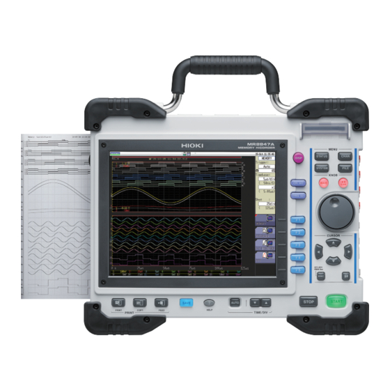
MR8847A
MR8847-51
MR8847-52
MR8847-53
MEMORY HiCORDER
Be sure to read this manual before using the instrument.
When using the instrument for the
first time
Part Names and Functions
Preparing for Measurement
Feb. 2019 Revised edition 3
MR8847G961-03 19-02H
p.16
p.25
Instruction Manual
Video
Scan this code to watch the
instructional video(s).
Carrier charges may apply.
Troubleshooting
Maintenance and Service
Error Messages
p.4
p.415
p.422
EN
Advertisement
Table of Contents

Subscribe to Our Youtube Channel
Related Manuals for Hioki MR8847-51


Summary of Contents for Hioki MR8847-51
- Page 1 MR8847A MR8847-51 MR8847-52 MR8847-53 Instruction Manual MEMORY HiCORDER Video Scan this code to watch the instructional video(s). Carrier charges may apply. Be sure to read this manual before using the instrument. p.4 When using the instrument for the Troubleshooting...
-
Page 3: Table Of Contents
Contents Contents Usage Index ..........1 3.4 Configuring Input Channels Introduction ..........2 Settings ......... 64 Verifying Package Contents ..... 3 3.4.1 Channel Setting Procedure ......65 3.4.2 Configuring Analog Channels Settings ..67 Safety Information ........4 3.4.3 Configuring Logic Channel Settings ...70 Operation Precautions ...... - Page 4 Contents Manually Printing Data by Viewing Waveforms Divided Pressing the PRINT Key Into Blocks ........153 (Selection Print) ......124 Setting the Print Density of the Advanced Functions Waveform ........126 6.5 Configuring the Printer Settings 127 Adding Comments ..... 156 Advanced Print Functions ..130 8.1.1 Adding, Displaying, and Printing the Title 6.6.1...
- Page 5 Contents 8.12 Saving Waveforms Registered 10.5 Printing the Numerical in Model U8793 onto a Storage Calculation Results ....238 Device .......... 200 10.6 Numerical Calculation Types 8.13 Setting Output Waveform and Descriptions ......239 Parameters on the Waveform Screen ......... 200 Waveform Calculation Function Setting the Trigger...
- Page 6 Contents 13.4 Configuring the Channel 16.2.1 Setting HTTP With the Instrument .... 338 16.2.2 Connecting the Computer to the settings ........282 Instrument With the Internet Browser ..339 13.5 Configuring the Screen Display 16.2.3 Operating the Instrument With the Settings ........283 Internet Browser ........340 13.5.1 Displaying the Running Spectrum ....
- Page 7 Contents Index Ind.1 18.3.2 Recorder Function ........377 18.3.3 X-Y Recorder Function ......378 18.3.4 FFT Function ........... 379 18.4 Other Functions ......380 18.5 File ..........385 18.6 Specifications of Modules ..387 18.6.1 Model 8966 Analog Unit ......387 18.6.2 Model 8967 Temp Unit ......388 18.6.3 Model 8968 High Resolution Unit .....
- Page 8 Contents...
-
Page 9: Usage Index
Usage Index Usage Index Basic measurement procedure 1 Installing the instrument Performing measurement in the automatic range setting (p. 76) (p. 25) Monitoring changes in input signals (p. 201) Installing the instrument Manually triggering the instrument (p. 216) Installing modules Entering comments (p. -
Page 10: Introduction
Introduction Introduction Thank you for purchasing the Hioki MR8847A Memory HiCorder (MR8847-51, MR8847-52, MR8847-53). To obtain maximum performance from the instrument, please read this manual first, and keep it handy for future reference. The optional clamps (p. Appx.13) collectively mean “clamp sensors.”... -
Page 11: Verifying Package Contents
In particular, check the accessories, panel switches, and connectors. If damage is evident, or if it fails to operate according to the specifications, contact your authorized Hioki distributor or reseller. Store the packaging in which the instrument was delivered, as you will need it when transporting the instrument. -
Page 12: Safety Information
Safety Information Safety Information This instrument and modules are designed to conform to IEC 61010 Safety Standards, and has been thoroughly tested for safety prior to shipment. However, using the instrument in a way not described in this manual may negate the provided safety features. Before using the instrument, be certain to carefully read the following safety notes: DANGER Mishandling during use could result in injury or death, as well as damage to the... - Page 13 Safety Information Symbols Affixed to the Instrument Indicates cautions and hazards. When the symbol is printed on the instrument, refer to the corresponding topic in the Instruction Manual. Indicates the ON side of the power switch. Indicates the OFF side of the power switch. Indicates a fuse.
- Page 14 Safety Information Accuracy We define measurement tolerances in terms of f.s. (full scale), rdg. (reading), and setting values with the following meanings: f.s. (maximum display value The maximum displayable value or scale length. or scale length) For this instrument, the maximum displayable value equals the numerical number of a presently set range (unit: V/div) multiplied by the number of di- visions (20) on the vertical axis.
-
Page 15: Operation Precautions
• Verify that it operates normally to ensure that no damage occurred during storage or shipping. If you find any damage, contact your authorized Hioki distributor or reseller. Installing the instrument and modules... - Page 16 If you have lost any screws or find that any screws are damaged, please contact your Hioki distributor for a replacement. CAUTION • To avoid damage to the instrument, protect it from physical shock when transporting and handling it.
- Page 17 Operation Precautions CAUTION Be careful not to cut yourself with the paper cutter. • Please use only the specified recording paper. Using non-specified paper may not only result in faulty printing, but printing may become impossible. • If the recording paper is skewed on the roller, paper jams may result. •...
- Page 18 Be sure to back up any important data saved on the built-in drive (SSD) or the removable storage device. • Use only CF cards sold by Hioki. (No adapter is required to insert a CF card into the instrument.) •...
- Page 19 Operation Precautions Before connecting cables DANGER When measuring power line voltage • Connect the connecting cables to only the secondary side of a breaker. Even if a short-circuit occurs on the secondary side of the breaker, the breaker will interrupt a short-circuit current. Do not connect them to the primary side of the breaker because an unrestricted current flow could damage the instrument and facilities if a short circuit occurs.
- Page 20 Operation Precautions Before connecting a logic probe to the measurement object DANGER To avoid an electric shock, a short-circuit, and damage to the instrument, observe the following precautions: • The ground pin in the logic connector (plug) of Model 9320-01 Logic Probe and Model 9327 Logic Probe are not isolated from the instrument’s ground (common ground).
- Page 21 Operation Precautions Before connecting the instrument to an external device DANGER To avoid electrical hazards and damage to the instrument, do not apply voltage exceeding the rated maximum to the external control terminals. I/O terminals Maximum input voltage Instrument START/EXT.IN1 −0.5 V to 7 V DC STOP/EXT.IN2 −0.5 V to 7 V DC...
- Page 22 • Keep discs inside a protective case and do not expose to direct sunlight, high temperatures, or high humidity. • Hioki is not liable for any issues your computer system experiences in the course of using this disc. When the instrument is not used for a long period •...
-
Page 23: Overview
Overview 1.1 Product Overview This instrument enables you to measure and analyze various waveforms with simple methods. You can use this instrument mainly for facility diagnosis, preventive maintenance, and troubleshooting. Sturdy body with easy-to-grasp You can install this portable instrument anywhere. handle installed Logic modules can measure You can take multiple measurements simultaneously. -
Page 24: Part Names And Functions
USB connector (Type A) Standard LOGIC terminals Connect a USB flash drive or a mouse. (p. 41) Connect optional Hioki logic probes. (p. 28) 100BASE-TX connector Various modules Connect a LAN cable. (p. 26), (p. 28) (p. - Page 25 Part Names and Functions Operation keys DISP STATUS Displays the waveform Displays the status screen. screen. CH.SET CHAN Displays the channel Displays the channel settings window on the screen. waveform screen (p. 64). TRIG.SET FILE Displays the trigger settings Displays the File screen. window on the waveform (p.
- Page 26 Part Names and Functions PRINT HELP Prints waveforms and lists. (p. 119) Displays help information. (p. 22) COPY AUTO Prints a screenshot. (p. 130) Starts measurement in the auto-range setting. (p. 76) FEED TIME/DIV Sets the timebase. Feeds paper. SAVE key (Lights up in blue while the instrument is accessing a storage device.) Saves data to a storage device.
-
Page 27: Screens Configuration
Screens Configuration 1.3 Screens Configuration The screens are configured as listed below. Pressing each of the keys listed below displays a corresponding screen or window. The waveform screen can display the trigger settings window, and the channel settings window. Waveform screen The display used to observe waveforms. -
Page 28: X84; Explanation Of Screen Contents
Screens Configuration Explanation of screen contents Waveform screen Title comment Trigger time Storage device icon Current date and time Shows a previously Shows the date Displays the status of Shows the current date entered title and time when storage devices. and time in the manner comment. -
Page 29: Basic Key Operation
Basic Key Operation 1.4 Basic Key Operation Press the CURSOR key and move the cursor to an item to be changed. Cursor Check the illustrations on the GUI and press the function key key) to change the settings. The function assigned to the key varies depending on the setting items. -
Page 30: Using The Help Key
Basic Key Operation 1.4.1 Using the HELP Key Pressing the HELP key displays a simple explanation of the item at the cursor position. You can also search the help messages for the information for which you are looking. Cursor position help Move the cursor to the item for which you want to display a help message. -
Page 31: Using Mouse To Enable Key Operation
Basic Key Operation 1.4.2 Using Mouse to Enable Key Operation Using a commercially available USB mouse enables you to operate the instrument in the manner similar to that with the keys on the instrument. • The instrument may not support some types of mouses. •... - Page 32 Basic Key Operation The operation keys of the instrument and the shortcut menu relate to each other as follows. To operate the functions assigned to the CH.SET, WAVE, and AB CSR keys and to configure those settings, click the icons displayed while a mouse is connected to the instrument. Icon Operation key CH.SET...
-
Page 33: Preparing For Measurement
Preparing for Measurement Procedure (p. 7) Install the instrument. Install or remove modules. (p. 26) (When adding or replacing modules) Connect logic probes to the LOGIC (p. 28) terminals. (When measuring logic signals) Connect connection cables to the (p. 28) modules. -
Page 34: Installing And Removing Modules
Installing and Removing Modules 2.1 Installing and Removing Modules Read “Handling the Instrument and Modules” (p. 8) carefully. Modules ordered with the instrument has already been installed in the instrument. Follow the procedures below to add, replace, or remove modules from the instrument. •... -
Page 35: X84; Channel Configuration
Installing and Removing Modules Channel configuration Modules are numbered beginning at the top, and channels are numbered beginning at the left of the module installed at the top. You can find out information about the modules installed in the instrument in the System Information (p. 429). -
Page 36: Attaching Connection Cables
Attaching Connection Cables 2.2 Attaching Connection Cables Read “Before connecting cables” (p. 11) carefully. For detailed precautions and instructions regarding connections, refer to the instruction manuals for your modules, connection cables, etc. Measuring voltage The following connection cables can be connected Applicable modules to the modules: •... - Page 37 Attaching Connection Cables Connecting cables to the BNC female terminals on modules Example: Model 8966 Analog Unit female connector Required item: Connection cables Connect the BNC male connector of the cable to a BNC female connector on the module. Connecting the cable Align the slots in the BNC male BNC male connector with the bayonet lugs...
- Page 38 Attaching Connection Cables Measuring Frequency, Number of Rotations, and Count Refer to (p. 29) for details about connecting a cable to the BNC female terminal. The following connection cables can be connected Applicable Module to the modules: • Model 8970 Freq Unit •...
- Page 39 Attaching Connection Cables Measuring temperature The following thermocouple can be connected to the Applicable Module module. • Model 8967 Temp Unit Thermocouple Connect thermocouple to (Compatible wire: from 0.4 mm terminal block to 1.2 mm in diameter) Connect a thermocouple to the terminal block on the module.
- Page 40 The following device can be connected to the Applicable Module module. • Model U8969 Strain Unit • Strain gauge transducer (Not available from Hioki) • Model 8969 Strain Unit Connect L9769 or 9769 Conversion Cable to the strain gauge transducer.
- Page 41 Attaching Connection Cables Connector pin-out Model L9769 Conversion Cable Model U8969 Strain Unit (Strain gauge transducer end) Applied voltage: bridge voltage of 2 V The metal shell is connected to The metal shell is connected to the GND of the instrument. the GND of the instrument.
- Page 42 Attaching Connection Cables Example: Connecting the strain gauge transducer to Model 8969 Strain Unit via Model 9769 Conversion Cable 8969 Strain Unit Required items: Model 9769 Conversion Cable, strain gauge transducer Connect Model 9769 to a connector on the module. Insert the connector of Model 9769 with the orange part facing upward.
- Page 43 Attaching Connection Cables Measuring current The following clamp sensors can be connected to Applicable Module the module. • Model 8971 Current Unit • Model 9272-10 Clamp On Sensor Connect a clump sensor to the connector • Model 9709, CT6862, CT6863, on the module via Model 9318 Conversion CT6865 AC/DC Current Sensor...
- Page 44 Attaching Connection Cables Measuring logic signals Read “Before connecting a logic probe to the measurement object” (p. 12) carefully. For more information about logic probe specifications, refer to the instruction manual of your logic probe. The following logic probes can be connected to the Applicable Module module.
- Page 45 Attaching Connection Cables Measuring voltage with a high degree of accuracy (digital voltmeter) The following lead can be connected to the module. Applicable Module • Model MR8990 Digital • Model L2200 Test Lead Voltmeter Unit (Maximum input voltage: 1000 V) Connect the test lead to the banana jacks on the module.
- Page 46 Attaching Connection Cables Measuring high voltage The following cables can be connected to the module. Applicable Module • Model L4940 Connection Cable Set • Model U8974 High Voltage (Maximum input voltage: 1000 V) Unit Connect the connection cable to the banana jacks on the module.
- Page 47 Attaching Connection Cables Outputting waveforms The following cables can be connected to the Applicable Modules module. • Model U8793 Arbitrary Waveform Generator Unit • Model L9795-01 Connection Cable (Electrical clips) • Model MR8790 Waveform Generator Unit Connect the connection cable to the output •...
- Page 48 Attaching Connection Cables Outputting a pulse waveform Required items: Commercially available cable Applicable Module (Half-pitch 50 pins) • Model MR8791 Pulse Generator Unit Connecting a connection cable to the output connector Output connector Required items: Commercially available cable Connect the connection cable to the output connector of the module.
-
Page 49: Preparing Storage Devices
Built-in drive * After formatting the drive, its capacity is decreased to less than 128 GB, which is an actually available capacity. The optional Model U8331 SSD Unit (factory option) is required. Hioki formatted the hard disk during the production process. - Page 50 Preparing Storage Devices Storage device How to insert devices, notes Memory (INT) • The memory installed in the instrument is available. Only settings files can be written in the memory. • Automatic writing of data is not possible. • Do not connect any devices other than USB flash drives. •...
-
Page 51: Formatting Storage Devices
Loading Recording Paper 2.3.2 Formatting Storage Devices The instrument can format CF cards, USB flash drives, the built-in drive, and the internal memory. Once they are formatted, the “HIOKI8847” folder is created. Note that formatting a storage device deletes all the information on the storage device, and the deleted information is unrecoverable. - Page 52 Loading Recording Paper Put the paper into the holder. Insert first the left side of the paper into the holder, and then, until the holder clicks, put the paper into the holder while pressing the paper leftward. Face the print side of the paper upward. If the paper is put in the holder without the paper roll axle installed, the printer cover cannot be open, resulting in damage to the printer.
-
Page 53: Supplying Power
Supplying Power 2.5 Supplying Power Read “Before turning on the instrument” (p. 12) carefully. 2.5.1 Connecting the Power Cord Procedure Right side Connect the power cord to the power inlet on the instrument. Plug the power cord into the mains outlet. 2.5.2 Connecting an Earthing Wire to the GND Terminal (Functional Earth Terminal) -
Page 54: Turning On And Off The Instrument
Supplying Power 2.5.3 Turning On and Off the Instrument Turning on the Instrument Right side Set the power switch in the on position ( The splash screen is displayed first, and then the Power switch waveform screen is displayed. : ON Before starting measurement To perform precise measurement, warm up the instrument about 30 minutes after turning on the instrument to stabilize the internal temperature of the modules. -
Page 55: Setting The Clock
Setting the Clock 2.6 Setting the Clock Set date and time for the built-in clock as follows. The clock has an automatic calendar with leap year correction and 24-hour format. The functions listed below make use of the clock. Ensure that the clock is set correctly before using these functions. -
Page 56: Adjusting The Zero Position (Zero-Adjustment)
Adjusting the Zero Position (zero-adjustment) 2.7 Adjusting the Zero Position (zero-adjustment) This operation compensates potential deflection of modules and sets the reference potential of the instrument to 0 V. The compensation operation is performed for all channels and ranges. Before performing zero-adjustment •... -
Page 57: Performing Calibration (When Model Mr8990 Is Installed)
Performing Calibration (When Model MR8990 is Installed) 2.8 Performing Calibration (When Model MR8990 is Installed) This operation calibrates the scale of MR8990 Digital Voltmeter Unit. The compensation operation is performed for all channels and ranges. Before performing calibration • Warm up the instrument for about 30 minutes after the power-on to stabilize the internal temperature of the modules, and then perform zero-adjustment. - Page 58 Performing Calibration (When Model MR8990 is Installed)
-
Page 59: Measurement
Measurement 3.1 Measurement Procedure 1 Inspecting the instrument before measurement Refer to “3.2 Inspecting the Instrument Before Measurement” (p. 53). 2 Configuring the basic measurement settings Refer to the following pages: Select a suitable recording method for “3.3.1 Measurement Functions” (p. 54) an object to be measured “3.3.2 Time Axis Range and Sampling Rate”... -
Page 60: Mr8847
Measurement Procedure 5 Starting measurement Refer to the following pages: “3.5 Starting and Stopping Measurement” (p. 73) “5 Saving/Loading Data and Managing Files” (p. 85) “6 Printing Data” (p. 119) “7.1 Reading Measured Values (Using Cursors A and B)” (p. 134) “7.3.2 Scrolling the Waveforms With the Jog Dial and Shuttle Ring”... -
Page 61: Inspecting The Instrument Before Measurement
3.2 Inspecting the Instrument Before Measurement Before using the instrument for the first time, verify that it operates normally to ensure that no damage occurred during storage or shipping. If you find any damage, contact your authorized Hioki distributor or reseller. -
Page 62: Setting Measurement Conditions
Setting Measurement Conditions 3.3 Setting Measurement Conditions This section describes how to set measurement conditions. The settings window displayed on the Waveform display enables you to configure basic settings conveniently while you are observing waveforms. The basic settings can also be configured on the [Status] sheet of the status screen How to open the settings window... - Page 63 Setting Measurement Conditions Values obtained by the recorder function While the recorder function is being used, the instrument obtains measured values at a previously set sampling rate and lets both the maximum and minimum values be a sampling data value during each of the sampling data periods.
-
Page 64: Timebase And Sampling Rate
Setting Measurement Conditions 3.3.2 Timebase and Sampling Rate The timebase setting defines a time length per division of the horizontal axis (time/div). The sampling setting defines an interval at which the instrument samples waveforms. (While the memory function is being used, the sampling rate appears, enclosed in parentheses, under the timebase box. - Page 65 Setting Measurement Conditions How to select the timebase Refer to the table below to set the timebase. For example, to measure a waveform with a frequency of 100 kHz, a maximum display frequency of between 200 kHz and 800 kHz should be selected according to the following table. When you want to set the maximum display frequency to 400 kHz, the timebase should be set to 10 µs/div.
- Page 66 Setting Measurement Conditions What is the maximum display frequency? To plot sine waves that allow you to observe those peaks on the LCD, the instrument needs to sample the waveforms at least 25 points per cycle. The maximum display frequency varies depending on the timebase setting.
- Page 67 Setting Measurement Conditions • The timebase and sampling rate can be set independently. The sampling rate is selected depending on the timebase setting. • As mentioned below, when the former timebase settings are selected, the instrument displays waveforms that are demagnified horizontally (in the time axis direction) at the latter scale size. 20 ms/div, ×1/2;...
-
Page 68: Setting The Recording Length (Number Of Divisions)
Freely specify a value in one division increments. Set the recording length. (Fixed Shot) Model MR8847-51 (Memory capacity: 64 MW) 25, 50, 100, 200, 500, 1,000, 2,000, 5,000, 10,000, 20,000 div 50,000 div (in 2/4/8-ch mode) 100,000 div (in 2/4-ch mode) - Page 69 Model MR8847-51 (Memory capacity: 64 MW) 25, 50, 100, 200, 500, 1,000, 2,000, 5,000, 10,000, 20,000 div Model MR8847-52 (Memory capacity: 256 MW)
- Page 70 When recording length is set to [Cont.] • The instrument saves data that is obtained during the period that lasts until the measurement terminates and has the maximum recording lengths (20,000 div for Model MR8847-51, 80,000 div for Model MR8847-52, and 160,000 div for Model MR8847-53).
-
Page 71: Setting Screen Layout
Setting Measurement Conditions 3.3.4 Setting Screen Layout You can lay out waveform displays of input signals on the waveform screen. This setting also applies to the printing setting. Selecting X-Y1 mode or X-Y4 mode plots X-Y composite curves. (This function can be used in the memory and X-Y recorder functions.) Refer to “7.4 Plotting X-Y Composite Curves”... -
Page 72: Configuring Input Channels Settings
Configuring Input Channels Settings <Example screen after assigning channels> Move the cursor to the [Graph] box. Select the display screen with respect to each channel. The graphs are numbered beginning from the top like Gr1, Gr2, Gr3. 3.4 Configuring Input Channels Settings Configuring analog and logic channels settings. -
Page 73: Channel Setting Procedure
Configuring Input Channels Settings 3.4.1 Channel Setting Procedure The procedure below shows how to configure the analog channels (CH1 through CH16) settings. 1 Configuring the settings of input and screen display Refer to the following pages: Configuring the input coupling setting (P. - Page 74 Configuring Input Channels Settings • Setting the input coupling set to GND disables the range settings because the waveforms seem to have no amplitude. • Filter attenuation may influence correct range settings. • When choosing trigger settings, set the vertical axis (voltage axis) range first. When you change the range after specifying the trigger, the trigger setting is changed.
-
Page 75: Configuring Analog Channels Settings
Configuring Input Channels Settings 3.4.2 Configuring Analog Channels Settings For information about specific settings for Model 8967 Temp Unit, 8969 Strain Unit, U8969 Strain Unit, 8970 Freq Unit, 8971 Current Unit, 8972 DC/RMS Unit, MR8990 Digital Voltmeter Unit, and U8974 High Voltage Unit, see “8.10 Setting Details of Modules”... - Page 76 Configuring Input Channels Settings 3. Input coupling You can set the input signal coupling method. Typically, select the DC coupling. DC (V) Measures the input signals including both DC components and AC components. (Default setting) Measures the input signal, including AC components only. DC AC ( components are rejected.
- Page 77 Configuring Input Channels Settings • The zero position setting merely change waveform positions, not applying any offsets to inputs signals. • The vertical axis (voltage axis) magnification/demagnification of waveforms is performed based on the zero position. • The zero position adjustment and the vertical axis (voltage axis) magnification/demagnification merely change displayable voltage ranges on the waveform screen.
-
Page 78: Configuring Logic Channel Settings
Configuring Input Channels Settings The magnification ratios enclosed in the brackets represent ranges of valid data. *: For Model 8967 Temp Unit, the valid range varies depending on thermocouples. For information about the minimum resolution, see the specifications of Model 8967 Temp Unit. 7. -
Page 79: Display Sheet
Configuring Input Channels Settings Displays no waveform. When [Save Channel] of the auto- [Display Ch], the instrument does not saving setting is set to save any data of this channel. Refer to “Select the channels to be saved.” (p. 93). Displays the waveform. - Page 80 Configuring Input Channels Settings • You can set the following display-related settings only with respect to each display sheet. Analog waveform: Display on/off, waveform color, magnification ratio, zero position, vernier, invert, graph, variable (on/off, upper and lower limits) Logic waveform: Display on/off, waveform color, display position, logic width X-Y curve: Display on/off, display color, X ch, Y ch, waveform calculation (X ch, Y ch)
-
Page 81: Starting And Stopping Measurement
Starting and Stopping Measurement 3.5 Starting and Stopping Measurement Procedure To display the screen Press the DISP key to display the waveform screen. To start measurement Press the START key to start measurement. • When measurement is started, waveform data displayed on the screen is cleared. •... - Page 82 Starting and Stopping Measurement Measurement and internal operations Two options of the measurement methods available: the normal measurement (starts measuring and recording waveforms at once) and trigger measurement (starts recording waveforms when trigger conditions are satisfied). In this manual, “Start of measurement” indicates the time when you press the START key, and “start of acquisition”...
- Page 83 Starting and Stopping Measurement Triggering the instrument repeatedly and recording phenomena before each trigger event Trigger mode: The specified pre-trigger wait period is recorded before each trigger event. Start measurement [Repeat] Recording START End of measurement With the pre-trigger Operation is enabled repeated from pre-triggering...
-
Page 84: Measurement In Automatic Range Setting (Auto-Range Function)
Measurement in Automatic Range Setting (Auto-Range Function) 3.6 Measurement in Automatic Range Setting (Auto-Range Function) This function is enabled only for measurement with the analog modules with the memory function enabled. When you press the AUTO key after inputting signals to an analog module and select [Auto Range], the horizontal axis range (timebase), vertical axis (voltage axis) range, and zero position are selected... - Page 85 Measurement in Automatic Range Setting (Auto-Range Function) • When measurement is started in the auto-range setting, the trigger output signal is output from the external control terminal block’s TRIG OUT terminal. Keep this in mind when performing auto-range measurement while using the trigger output terminal. •...
- Page 86 Measurement in Automatic Range Setting (Auto-Range Function)
-
Page 87: X-Y Recorder
X-Y Recorder • You can plot X-Y composite curves each of which presents the relationship between an input signal and another in real time. • Since the instrument writes the data of plotted curves in the memory, it can save the data as files as well as print the curves. -
Page 88: Measurement Procedure
Measurement procedure 4.1 Measurement procedure 1 Inspecting the instrument before measurement Refer to “3.2 Inspecting the Instrument Before Measurement” (p. 5 3). 2 Configuring the basic measurement settings Refer to the following pages: Setting the measurement function “Measurement function” (p. 8 1) to the X-Y recorder Setting the sampling rate “Sampling”... -
Page 89: Setting Measurement Conditions
Setting Measurement Conditions 4.2 Setting Measurement Conditions To set the measurement conditions, press the STATUS key to display the status screen, and then select [Status] sheet. (The measurement functions and sampling rates can also be set on the waveform screen.) Setting items Measurement Set the measurement function to... -
Page 90: Starting And Stopping Measurement
Starting and Stopping Measurement To choose channels used to plot X-Y composite curves Refer to “7.4 Plotting X-Y Composite Curves” (p. 1 44). 4.3 Starting and Stopping Measurement Press the DISP key to go to the waveform screen. Start measurement. START Press the key to start measurement. - Page 91 Starting and Stopping Measurement Move the cursor to the [Player] box. Clear Clears only the displayed X-Y composite curves. (The instrument does not discard the waveform data written in the memory.) Redraw Redraws the X-Y composite curves. The X-Y composite curve display conditions can also be changed for plotting the curves again.
-
Page 92: Observing X-Y Composite Curves
Observing X-Y Composite Curves 4.4 Observing X-Y Composite Curves Up to 4,000,000 samples of waveform data are written in the memory, and you can observe those measured values using Cursors A and B. (p. 134) The bar at the top of the screen indicates the amount of the occupied memory. When the number of samples reaches 4 million, the sign [OVER] appears... -
Page 93: Saving/Loading Data And Managing Files
Saving/Loading Data and Managing Files This chapter explains how to save and load data and manage files. [File Save] Before saving data, configure the save settings on the sheet of the system screen. File screen allows you to load data and manage files. To display the [File Save] sheet... - Page 94 To display the file screen Indicated the order in which the files are sorted. △: Ascending order ▽: Descending order Press [FILE] key. The selected file is indicated by the flashing cursor. Press Left/Right CURSOR key to move between folder levels.
-
Page 95: Data That Can Be Saved And Loaded
Data That Can Be Saved and Loaded 5.1 Data That Can Be Saved and Loaded : Yes, –: No Save File Computer- File type Icon File extension and description Load format readable Auto. Manual Settings data (measurement Settings data Binary –... - Page 96 Data That Can Be Saved and Loaded To load the data, which is saved with the memory division enabled, of entire blocks at once Save measured data in the [All blocks] setting. A directory including waveform data for each block and index data (SEQ) is automatically created.
-
Page 97: Saving Data
Saving Data 5.2 Saving Data 5.2.1 Save Types and Setting Procedure There are basically three types of save operations. To save data automatically To save data manually by pressing the SAVE key (p. 97) during measurement (p. 90) To save data after To save data immediately selecting items Auto-saving... -
Page 98: Automatically Saving Waveforms
Saving Data 5.2.2 Automatically Saving Waveforms The instrument automatically saves the waveform data as files every time it writes the recording length of the waveform data in the memory. Set the save destination and items to be saved before starting measurement. - Page 99 Saving Data Set the save destination. Move the cursor to the [Save To] box and select [Edit]. Up/down To select a storage device CURSOR The folder dialog box is displayed (at the bottom right). To open the Right Move the cursor to a device to be set as the save CURSOR lower level folder [Confirm]...
- Page 100 Saving Data Specify the action when a file with the same name exists in the target folder. Move the cursor to the [Same Name] box. Auto When no files with the same name exist, the instrument gives the predetermined name to a file and saves it.
- Page 101 Every other data point is saved. The number of data points is reduced to 1/2 of the original amount. Save destination Data can also be automatically saved on a USB flash drive; however, we recommend using Hioki’s optional CF card instead for data protection. Select the channels to be saved.
- Page 102 Saving Data Set the save method when the space of the storage device is insufficient. Move the cursor to the [Save method] box. Normal Stops the automatic saving when the storage Save device is full. Delete Deletes old files and continue the automatic Save saving when the storage device is full.
- Page 103 Saving Data Auto-saving operations (When the save destination is set to a storage device) Example 1: Saving files in the topmost directory of the storage device (the instrument creates the “ HIOKI8847 ” folder and saves files in the folder.) 0000AUTO.MEM Save to CF:\HIOKI8847...
- Page 104 The instrument gives the names in the previously- determined formats to the destination folders and files, and then saves them as follows: Waveform files Specified folder WAVE123015.MEM 192.168.1.1 15-10-10 HIOKI 9333 WAVE123245.MEM The folder name is the IP 15-10-11 WAVE123245.TXT address of the instrument.
-
Page 105: Saving Data Selectively (Save Key)
Saving Data 5.2.3 Saving Data Selectively (SAVE Key) SAVE To save file instantly, by pressing the key, you need to specify the items to be saved beforehand. You can save the following types of data: Setting data, waveform data, display images, waveform images, and numerical calculation results. - Page 106 Saving Data Set the save destination. Move the cursor to the [Save to] box, and select [Edit]. To select a Up/down storage device CURSOR To open the The folder dialog box is displayed (See the bottom figure Right lower level on the right).
- Page 107 Saving Data Specify the action when a file with the same name exists in the target folder. Move the cursor to the [Same Name] box. Auto When no files with the same name exist, the instrument gives the predetermined name to a file and saves it.
- Page 108 Saving Data Set the items to be saved. Move the cursor to the [Save Type] box. Setting Saves the settings data. Wave Saves waveform data in binary format. Binary Select this option to reload the waveforms with the instrument. Wave Saves waveform data in text format.
- Page 109 Saving Data (When [Save Type] is set to [Wave Binary] [Wave Text]) Move the cursor to the [Save Area] box. Whole Saves the entire data written in the memory. Wave (Default setting) Saves the data within the range between Wave Cursors A and B.
- Page 110 Saving Data Save Settings Description types Output (All, 1 through 250) Waveform screen File Specifies the number of files to be (Print saved. image) To specify a print range, open the [Printer] sheet using the system screen, and set the print range setting to [A-B Wave].
-
Page 111: Saving Waveform Outputting Data To A Storage Device
Saving Data 5.2.4 Saving Waveform Outputting Data to a Storage Device You can save pulse pattern data registered in Model MR8791, arbitrary waveform data registered in Model U8793, or program data in a storage device. Before attempting to save the data, make sure that a storage device is inserted and the destination to save is correctly specified. -
Page 112: Loading Data
Loading Data 5.3 Loading Data You can load the data saved on a storage device or in the internal memory of the instrument. Data loading procedure Before attempting to save the data, make sure that a storage device is inserted, and the save destination is correctly specified. - Page 113 Loading Data Procedure To display the screen FILE Press the key to display the file screen. To load a text comment Press the SYSTEM key to display the [Printer] sheet on the system screen. Move the cursor to the [Text Comment] box, and select [Before Wave]...
- Page 114 Loading Data To load waveform files in a bundle Loading the following index files permits waveform files to be loaded in a batch. The following settings create index files along with waveform files. Extension Explanation Divided files are loaded in a batch. (To create index files, on the system screen, select the [File Save] sheet, enter the dividing size...
-
Page 115: Automatically Loading Settings (Auto-Setup Function)
Automatically Loading Settings (Auto-setup Function) 5.4 Automatically Loading Settings (Auto-setup Function) The saving settings described below permit themselves to be automatically loaded at startup. The auto-setup function supports the STARTUP file saved on a CF card only. When the STARTUP file is saved on the built-in drive, USB flash drive, or RAM (internal memory), it is not be referred. -
Page 116: Managing Files
Managing Files 5.5 Managing Files Press the FILE key to display the file screen. The file screen allows you to manage data saved in storage devices. Select a file on the file list with the CURSOR key. Before performing an operation, insert a storage device (except for the optional built-in drive). If no storage device is inserted, the [NO FILE] message appears on the file list of the file screen. -
Page 117: Saving Data
Managing Files 5.5.1 Saving Data You can save settings data, waveform data, and waveform generation data in a storage device. The instrument saves data in the folder indicated by the cursor. You can specify a range using Cursors A and B and save a portion of waveform data. Procedure To display the screen Press the... - Page 118 Managing Files Specify the action when a file with the same name exists in the target folder. Move the cursor to the [Same Name] box. Auto When no files with the same name exist, the instrument gives the predetermined name to a file and saves it. When another file with the same name exists, the instrument gives the name beginning with a 4-digit number to a file and saves it (default setting).
- Page 119 Managing Files Execute the save operation. Select [Exec]. To cancel the file saving action, select [Cancel]. File name The maximum number of characters for [Save Name] is 123. The maximum path length including file name is 255 in characters. Division save •...
-
Page 120: Checking The Contents In A Folder (Opening A Folder)
Managing Files 5.5.2 Checking the Contents in a Folder (Opening a Folder) Opening a folder enables you to observe its contents. (The instrument displays the contents of the folder.) Procedure To display the screen Press the FILE key to display the file screen. To change storage devices (p. -
Page 121: Deleting Files And Folders
Managing Files 5.5.4 Deleting Files and Folders Follow this procedure to delete files or folders. Procedure To display the screen Press the FILE key to display the file screen. To change storage devices (p. 86) Select the file or folder you want to delete. Select the icon. -
Page 122: Sorting Files
Managing Files 5.5.5 Sorting Files You can sort files in the selected order. Procedure To display the screen Press the FILE key to display the file screen. To change storage devices (p. 86) Select [Sort], and then select a sort criterion in the [Type] box. -
Page 123: Renaming Files And Folders
Managing Files 5.5.6 Renaming Files and Folders You can rename files and folders. Procedure To display the screen Press the FILE key to display the file screen. To change storage devices (p. 86) Select the file or folder you want to rename. Select the icon. -
Page 124: Copying A File Into A Specified Folder
Managing Files 5.5.7 Copying a File Into a Specified Folder You can copy files into the specified folders. Procedure To display the screen Press the FILE key to display the file screen. (p. 86) Move the cursor to the file you want to copy. Select Select [Copy]. -
Page 125: Printing The File Table
Managing Files 5.5.8 Printing the File Table You can print the file table displayed on the file list of the file screen. The file table containing all displayed items are printed. Only folder names are printed. Any other information on the contents contained in folders is not printed. Before printing file tables, make sure the recording paper is loaded correctly. - Page 126 Managing Files...
-
Page 127: Printing Data
Printing Data [Printer] sheet enables you to set the print method and detailed printer options. To display the [Printer] sheet Pressing the PRINT switches the sheets to be displayed in the following order: [Environment] [Init] [File Save] [Printer] [Interface] What you can do on the [Printer] sheet Setting the print methods Configuring the printer settings Refer to the following pages:... -
Page 128: Print Type And Procedure
Print Type and Procedure 6.1 Print Type and Procedure There are three basic types of printing. Printing data after selecting Printing data by pressing Printing data automatically contents to be printed after PRINT key after during measurement measurement. measurement. Auto-printing Selection Print Quick Print When the memory function* is... -
Page 129: Setting Auto-Printing
Setting Auto-printing 6.2 Setting Auto-printing This function can be used in the memory, recorder, and FFT functions. These settings must be set before starting measurement. When you press the START key to start measurement, measured data will be printed automatically. When using the printer output, make sure that the recording paper is loaded correctly. - Page 130 Setting Auto-printing Set the print margins between two actions of the automatic print Move the cursor to the [Feed] box. Leaves a margin. (Default setting) Does not leave margins.* * Leaves a 2-mm-width margin. The setting in the [Feed] box is also applicable for normal printing. Check the measurement conditions and start measurement.
- Page 131 Setting Auto-printing [Output] is set to [LAN], real-time printing is disabled. The instrument with the auto-printing setting When prints the data automatically after the recording length of the data is written in the memory regardless of the timebase setting. Printing numerical calculation results simultaneously On the status screen, select the [Num Calc] sheet, and set...
-
Page 132: Manually Printing Data By Pressing The Print Key (Selection Print)
Manually Printing Data by Pressing the PRINT Key (Selection Print) 6.3 Manually Printing Data by Pressing the PRINT Key (Selection Print) PRINT Pressing the key on the waveform screen enables you to specify the print range and data type, and then start printing of the data. This action can prevent inadvertent printing due to operator error. - Page 133 Manually Printing Data by Pressing the PRINT Key (Selection Print) Start and then stop measurement. Press the START key to start measurement. Press the STOP key to stop the measurement in progress. Printing is not possible during measurement. Stop the measurement in progress before start printing.
-
Page 134: Setting The Print Density Of The Waveform
Setting the Print Density of the Waveform 6.4 Setting the Print Density of the Waveform You can set the printing density of the waveform with respect to each channel. Procedure To display the screen Press the CHAN key to open the channel screen, and then select the [Unit List] sheet or [Each Ch]... -
Page 135: Configuring The Printer Settings
Configuring the Printer Settings 6.5 Configuring the Printer Settings Configure the printer settings on the [Printer] sheet of the system screen. Printer settings To display the screen Press the SYSTEM key and then select the [Printer] sheet. (p. 130) (p. 132) Select the print speed (quality). - Page 136 Configuring the Printer Settings (p. 130) (p. 132) Select the horizontal axis (time axis) Time* Prints waveforms on the scale markings display value. based on the time from the trigger point (the unit is fixed). (Default setting) Move the cursor to the [Time Value] box.
- Page 137 Configuring the Printer Settings Set the upper and lower limit value. Prints waveforms without upper and lower Move the cursor to the [Up/Low Print] box. limits. (Default setting) <Print Example> Prints waveforms with upper and lower limits. Upper and lower limits Set the zero-position comment.
-
Page 138: Advanced Print Functions
Advanced Print Functions 6.6 Advanced Print Functions You can print the screenshot of the screen display, reports, and lists. 6.6.1 Printing the Screenshot Press COPY key while the screen you want to print is displayed. The screenshot is printed. The GUI section can be included on the print. Configuring the GUI print setting To display the screen SYSTEM... - Page 139 Advanced Print Functions Settings <Print Example> Title While holding down the FEED key, press the COPY key. To stop the printing action before it has finished Press the STOP key. Upper and Channel lower limits Values at Cursors A Cursors A and B and B...
-
Page 140: Printing A List
Advanced Print Functions 6.6.3 Printing a List You can print lists of function status information and channel setting information. The items included in the printed list are the same as those in the list function setting. Refer to “Configure the list setting” (p. 128). Press the PRINT key while any screen other than the waveform and file screen is displayed. -
Page 141: Monitoring And Analyzing Waveforms On The Waveform Screen
Monitoring and Analyzing Waveforms on the Waveform Screen Analytical operations such as the display magnification, display demagnification, and search are available on the waveform screen. The measurement conditions or other configuration can also be changed on this screen. To display the waveform screen Cursor A Cursor B Scroll bar... -
Page 142: Reading Measured Values (Using Cursors A And B)
Reading Measured Values (Using Cursors A and B) 7.1 Reading Measured Values (Using Cursors A and • You can read time lag, frequency, and potential difference (and scaling values when the scaling is enabled) as numerical values using Cursors A and B on the waveform screen. The cursors also enable you to specify ranges used for calculating values and the X-Y composite curve printing. - Page 143 Reading Measured Values (Using Cursors A and B) Move Cursors A and B with the jog dial or shuttle ring. (When the AB CSR key LED is on, you can move the cursors with the jog dial or the shuttle ring. Pressing any key other than the AB CSR key closes the setup screen.)
- Page 144 Reading Measured Values (Using Cursors A and B) Reading measured values on the waveform screen (in Single, Dual, Quad, and Oct mode) To display the screen DISP Press the key to display the waveform screen. <Screen display (for time axis cursor)> Values at Values between Cursor A Cursor B...
- Page 145 Reading Measured Values (Using Cursors A and B) • When using the external sampling, the value t represents the number of samples. • When the voltage range is changed during measurement using the recorder function or X-Y recorder function, measured values are acquired by tracing the waveforms in the range settings when the measurement was stopped.
- Page 146 Reading Measured Values (Using Cursors A and B) Reading measured values on the waveform screen (in Single, Dual, Quad, and Oct mode) To display the screen DISP Press the key to display the waveform screen. <Screen display (X-axis cursor)> X-Y composite curve of waveforms obtained Values at through CH1 and CH2 Cursor A...
-
Page 147: Specifying The Waveform Range (Cursors A And B)
Specifying the Waveform Range (Cursors A and B) 7.2 Specifying the Waveform Range (Cursors A and When the waveforms are displayed on the voltage-time graph, you can specify the range with the time axis cursor or trace cursor. The specified range is applicable for saving files, printing waveforms, plotting X-Y composite curves, and performing the numerical calculation. - Page 148 The maximum measured data the instrument can record internally is as follows: MR8847-51: Up to 20,000 div MR8847-52: Up to 80,000 div MR8847-53: Up to 160,000 div...
-
Page 149: Moving The Waveform Display Position
Moving the Waveform Display Position 7.3 Moving the Waveform Display Position This function can be used in the memory and recorder functions. 7.3.1 Display Position The scroll bar provides the relative position and size of the displayed portion of the waveforms within the entire recording length of the waveforms. - Page 150 Moving the Waveform Display Position To see previously obtained waveforms in roll mode Rotating the jog dial or shuttle ring allows you to observe the previously obtained waveforms during measurement. To redisplay the waveforms, select [Scroll].
-
Page 151: Changing Position (Jump Function)
Moving the Waveform Display Position 7.3.3 Changing Position (Jump Function) You can specify the portion of the waveforms and display them immediately. You can choose a display location from the following: • Trigger point • Positions of Cursor A and B •... -
Page 152: Plotting X-Y Composite Curves
Plotting X-Y Composite Curves 7.4 Plotting X-Y Composite Curves This function can be used in the memory and X-Y recorder functions. • To plot X-Y composite curves, display the status screen, follow the procedure below: (1) Select the [Status] sheet. [Format] (2) Set to X-Y1 screen or X-Y4 screen. - Page 153 Plotting X-Y Composite Curves Procedure To display the screen Press the DISP key to display the waveform screen, and then press the CH.SET key to display the X-Y settings window. Set the waveform color used in the graph Displays no waveform. When [Save display.
-
Page 154: Magnifying And Demagnifying
Magnifying and Demagnifying Waveforms 7.5 Magnifying and Demagnifying Waveforms 7.5.1 Magnifying and Demagnifying Waveforms Horizontally (in the Time Axis Direction) This function can be used in the memory and recorder functions. (However, with the recorder function, waveform magnification is not available.) Magnifying waveforms horizontally (in the time axis direction) enables you to observe data in detail. -
Page 155: Zoom Function (Horizontally Magnifying A Part Of Waveforms [In The Time Axis Direction])
Magnifying and Demagnifying Waveforms 7.5.2 Zoom Function (Horizontally Magnifying a Part of Waveforms [in the time axis direction]) This function can be used in the memory function only. You can display partly magnified (zoomed-in) waveforms together on the horizontally split dual displays with the normal waveforms. - Page 156 Magnifying and Demagnifying Waveforms Move the cursor to the [Zoom Mag] box. Select [Zoom On]. The zoom function is enabled, and the screen is horizontally split into two: the upper and lower screens. (Upper: waveforms magnified in the specified ratio; lower: partly magnified (zoomed) waveforms) Select the zoom-in ratio.
-
Page 157: Magnifying/Demagnifying The Waveforms Vertically (In The Voltage Axis Direction)
Magnifying and Demagnifying Waveforms Normal display Zoomed display 7.5.3 Magnifying/demagnifying the Waveforms Vertically (in the Voltage Axis Direction) This function can be used in the memory and recorder functions. You can magnify and demagnify the waveforms vertically (in the voltage axis direction) for the display or printing with respect to each channel. -
Page 158: Monitoring Input Levels (Level Monitor)
Monitoring Input Levels (Level Monitor) 7.6 Monitoring Input Levels (Level Monitor) 7.6.1 Level Monitor You can monitor all input waveform levels in real time. You can display analog channels and logic channels at a time. Procedure To display the menu DISP Press the key to display the display menu. -
Page 159: Numerical Value Monitor
Monitoring Input Levels (Level Monitor) 7.6.2 Numerical Value Monitor You can read input signals as numerical values displayed in the same way as digital multimeters (DMMs). Procedure To display the screen Press the DISP key twice. Display menu When the mouse is connected, clicking the [DMM] icon displayed at the upper right of waveform screen allows numerical value (DMM display) to be... -
Page 160: Switching The Waveform Screen Display (Display Menu)
Switching the Waveform Screen Display (Display Menu) 7.7 Switching the Waveform Screen Display (Display Menu) You can display the additional information such as upper and lower limit values and comments using the display menu. You can also set the waveform display width. Refer to “7.6.1 Level Monitor”... -
Page 161: Switching The Sheet To Be Displayed
Viewing Waveforms Divided Into Blocks 7.7.4 Switching the Sheet to Be Displayed [↑] [↓] Select between to switch the sheet to be displayed. You can specify the settings with respect to each displayed sheet on the unit list tab of the channel settings window. - Page 162 Viewing Waveforms Divided Into Blocks...
-
Page 163: Advanced Functions
Advanced Functions Advanced measurement and settings Adding comments (p. 156) • Displaying waveforms during the recording (p. 163) Converting input values (scaling) (p. 167) • Overlay waveforms with the waveforms recorded before (p. 164) Freely setting the waveform display Detailed module settings (p. 180) (p. -
Page 164: Adding Comments
Adding Comments 8.1 Adding Comments 8.1.1 Adding, Displaying, and Printing the Title Comment Entering a title comment enables itself to be displayed at the top of the waveform screen and to be printed on the recording paper. (Available number of characters: up to 40) Refer to “6.6.2 Printing Reports (A4-Sized Print)”... -
Page 165: Adding, Displaying, And Printing The Channel Comments
Adding Comments 8.1.2 Adding, Displaying, and Printing the Channel Comments Entering comments with respect to each channel enables you to confirm the comments of each channel on the screen. The comments can also be printed on the recording paper. (Available number of characters: up to 40) To copy the comment to another channel You can copy the comment on the... - Page 166 Adding Comments To select the comment from the previously registered terms Pressing the WAVE key after activating the text input displays the list of previously registered terms. It is also possible to select words from the previously entered analog channel comments (history list).
-
Page 167: Entering Alphanumeric Characters
Adding Comments 8.1.3 Entering Alphanumeric Characters Move the cursor to the setting item for which you wish to enter text and choose the content with the key. Entering texts Move the cursor to the comment field and select [Enter Char]. The virtual keyboard is displayed. - Page 168 Adding Comments Select [Confirm] to confirm the entry. The virtual keyboard is closed. Press the key to suspend the entering. (Pressing the key again closes the virtual keyboard.) To enter units and symbols Some characters are saved using alternative characters. (When saved as numerical calculation results or in text format) Ω...
- Page 169 Adding Comments Entering texts from the term list or history list While the virtual keyboard is being displayed, pressing the WAVE key displays the term list, and pressing AB CSR key displays the history list. They are available to enter the previously registered terms or the previously entered terms. Move the cursor to the comment box and select [Enter Char].
- Page 170 Adding Comments Entering numerals by increasing and decreasing them Move the cursor to the numeric input box and select [Up-Down]. The virtual keyboard for digit input is displayed. Enter numerals using the virtual keyboard. (Press to move the digit. Press to increase and decrease the value, respectively.) Select...
-
Page 171: Displaying Waveforms During The Writing In The Memory Simultaneously (Roll Mode)
Displaying Waveforms During the Writing in the Memory Simultaneously (Roll Mode) 8.2 Displaying Waveforms During the Writing in the Memory Simultaneously (Roll Mode) This function can be used in the memory function only. You can display and print the waveforms at the same time as the data is acquired (with the auto-print set to on). -
Page 172: Overlaying New Waveforms With Past Waveforms
Overlaying New Waveforms With Past Waveforms In addition, while evaluating data by calculating the numerical values, the instrument automatically prints the waveforms based on the evaluation conditions on completion of the numerical calculation. When the roll mode function is set to [Off] Since the instrument displays the waveforms after storing the entire recording length of the data, it takes a long time after starting measurement until displaying the waveforms with a relatively slower sampling. - Page 173 Overlaying New Waveforms With Past Waveforms Overlaying the waveforms manually (Leaving any waveforms to be displayed on the screen) To display the screen Press the DISP key to display the waveform screen. Move the cursor to the [Overlay] box. Overlay Leaves the waveforms written in the memory on the key) screen.
-
Page 174: Setting Channels To Be Used (Extending The Recording Length)
Setting Channels to Be Used (Extending the Recording Length) 8.4 Setting Channels to Be Used (Extending the Recording Length) This function can be used in the memory function only. Select the analog and logic channels to use. The fewer the number of the channels in use is, the longer the recording length becomes. Minimizing the number of channels to be used allows the storage memory to be allocated to the channels. -
Page 175: Converting Input Values (Scaling Function)
Converting Input Values (Scaling Function) 8.5 Converting Input Values (Scaling Function) About the scaling function The scaling function enables you to convert the measured voltage output from measurement devices such as sensors to physical quantities of measurement targets. Hereafter, “scale” refers to converting numerical values using the scaling function. Gauge scales, scaled values (upper and lower limits of the vertical axis [voltage axis]), and measured values at Cursors A and B are expressed as scaled values in terms of the specified units. - Page 176 Converting Input Values (Scaling Function) When the conversion ratio setting is changed, V and V set as two points used for conversion do not change, whereas the values for A and A change. Procedure To display the screen Press the CHAN key to display the channel screen, and then select the [Each Ch]...
-
Page 177: Example Of Scaling Settings
Converting Input Values (Scaling Function) To enter the current input values in the [Input P1] [Input P2] boxes with no change. [Monitor Val]. Select To reset the scaling settings Move the cursor to the [Set] box and select [Reset]. To copy the scaling setting to another channel Display the channel screen, and select the [Scaling] sheet. - Page 178 Converting Input Values (Scaling Function) To select the clamp sensor 1. Move the cursor to the [Clamp] and select [Select] The cursor moves to the [Model] box. 2. Select [9000〜] The cursor moves to the [Clamp] box. 3. Select [9018-50] from the clamp list by pressing the keys, and select [Confirm].
- Page 179 Converting Input Values (Scaling Function) Scaling signals from the strain gauge transducer enabled them to be displayed as physical values. Values at the Cursors A and B and gauges are displayed and printed as physical values. Refer to Gauge (p. 128) and Values at Cursors A and B (p.
- Page 180 Converting Input Values (Scaling Function) When the strain gauge transducer’s inspection record provides the calibration factor [Method] on the [Scaling] sheet to [Ratio]. Example 3 To display the data measured with the strain gauge transducer with a calibration factor of −6 0.001442 G / 1 ×...
- Page 181 Converting Input Values (Scaling Function) Using the decibel values To convert 40 dB of input into 60 dB Example 5 For scaling values, set [Method] to [Ratio]. Move the cursor to the conversion rate setting. Select [dB Scaling] in the function keys. Enter 40 dB in the entry field and 60 dB in the physical quantity field.
-
Page 182: Setting The Waveform Position (Variable Function)
Setting the Waveform Position (Variable Function) 8.6 Setting the Waveform Position (Variable Function) You can freely set the waveform height and display position along the vertical axis (voltage axis). Precautions when using the variable function • Verify that the proper vertical axis (voltage axis) range is set for the input signal. •... - Page 183 Setting the Waveform Position (Variable Function) Setting the variable function with respect to each channel Procedure To display the screen Press the CHAN key to display the channel screen, and then select the [Each Ch] sheet. Enable the variable function. Move the cursor to the [Variable] box, and select [On].
- Page 184 Setting the Waveform Position (Variable Function) Setting the variable function while the waveforms obtained through all of the channels are being displayed Procedure To display the screen Press the DISP key to display the waveform screen, and then press the CH.SET key to display the display range window.
-
Page 185: Fine-Adjusting Input Values (Vernier Function)
Fine-Adjusting Input Values (Vernier Function) 8.7 Fine-Adjusting Input Values (Vernier Function) You can fine-adjust the input voltage freely on the waveform screen. When recording physical values such as noise, temperature, and acceleration with sensors, you can adjust those amplitudes, facilitating calibration. -
Page 186: Inverting The Waveform (Invert Function)
Inverting the Waveform (Invert Function) 8.8 Inverting the Waveform (Invert Function) This function can be used for analog channels only. You can turn over the waveforms upside down by inverting signs. <Example> The invert function is useful when you want to let pulling force of a spring be negative and pushing force be positive;... -
Page 187: Copying Settings To Other Channels (Copy Function)
Copying Settings to Other Channels (Copy Function) 8.9 Copying Settings to Other Channels (Copy Function) You can copy a setting to other channels and calculation numbers (when using the FFT function) on the following screens: • Channel settings window • Display range window •... -
Page 188: Setting Details Of Modules
Setting Details of Modules 8.10 Setting Details of Modules You can configure detailed settings with respect to each module on the [Each Ch] sheet of the channel screen. How to display the [Each Ch] sheet and select channels Shows the channel number and channel position. -
Page 189: Setting The Anti-Aliasing Filter (A.a.f.) (Model 8968 High Resolution Unit)
Setting Details of Modules When Model 8970 Freq Unit is allocated to CH1 through CH4, using the standard logic channels LA through LD prohibits the modules of corresponding channels from being used. When Model MR8990 Digital Voltmeter Unit, U8793 Arbitrary Waveform Generator Unit, MR8790 Waveform Generator Unit, or MR8791 Pulse Generator Unit is allocated to CH1 through CH4, the corresponding standard logic channels described in the above table cannot be used. -
Page 190: Setting Model 8967 Temp Unit
Setting Details of Modules 8.10.3 Setting Model 8967 Temp Unit Refer to “How to display the [Each Ch] sheet and select channels” (p. 180). Mode Choose an option depending on the type of thermocouple to be used. Selection Measurement input range Selection Measurement input range Temp-K... -
Page 191: Setting Model 8969 And U8969 Strain Unit
Setting Details of Modules 8.10.4 Setting Model 8969 and U8969 Strain Unit The Model 8969 or U8969 Strain Unit can perform the auto-balance. Executing the auto-balance adjusts the reference output level of the transducer to the specified zero position. This function can be used for Model 8969 or U8969 Strain Unit only. The instrument describes Model U8969 as “8969.”... -
Page 192: Setting Model 8970 Freq Unit
Setting Details of Modules 8.10.5 Setting Model 8970 Freq Unit When the standard logic (LA, LB, LC, LD, LE, LF, LG, and LH) is displayed, Model 8970 Freq Unit installed as modules 1, 2, 9, or 10 cannot be used. Refer to “How to display the [Each Ch] sheet and select channels”... - Page 193 Setting Details of Modules To prevent measurement errors due to noise, the hysteresis width that is approximately 3% of the input voltage is tolerated for the threshold. [VRange] ±10V], it is approximately ±0.3 V.) (When is set to Set a threshold allowing for tolerance exceeding the hysteresis width relative to the peak voltage. Slope The instrument detects the waveform when the waveform crosses the specified level in the direction specified here, which is used in each measurement mode.
- Page 194 Setting Details of Modules Refer to “How to display the [Each Ch] sheet and select channels” (p. 180). Level You can use this setting only when setting [Mode] [Pulse Width] or [Duty]. For the pulse width measurement and duty ratio measurement, you can select whether to detect the parts that are above the threshold level or those that are below the level.
-
Page 195: Setting Model 8971 Current Unit
Setting Details of Modules 8.10.6 Setting Model 8971 Current Unit You do not have to change the setting because the setting is configured when the clamp sensor is automatically recognized. Refer to “How to display the [Each Ch] sheet and select channels” (p. 180). Mode 20A/2V Sets this option when Model 9272-10 (20 A range), 9277, or CT6841... -
Page 196: Setting Model Mr8990 Digital Voltmeter Unit
Setting Details of Modules 8.10.8 Setting Model MR8990 Digital Voltmeter Unit • Installing the Model MR8990 Digital Voltmeter Unit as Unit 1 and Unit 2 disables the standard logic channels. • The resolution of the data measured by the recorder function is 16 bits. •... -
Page 197: Setting Model U8974 High Voltage Unit
Setting Details of Modules • It takes approximately 150 ms to calibrate the MR8990. During this period, no measurement is performed. • If the channels are synchronized with each other, the signal that interrupts the integration is sent to each module at the start of measurement; thus, the instrument has to wait until the first integration finishes. -
Page 198: Setting Mr8790 Waveform Generator Unit
Setting Details of Modules 8.10.10 Setting MR8790 Waveform Generator Unit The channels with Model MR8790 installed cannot be used for measurement. Refer to “How to display the [Each Ch] sheet and select channels” (p. 180). Type Selects the waveform types. Outputs a DC signal (Default setting) Sine Outputs a sine wave... - Page 199 Setting Details of Modules Offset For DC output: Sets a DC voltage. For sine wave output: Sets an offset voltage. The output voltage range the accuracy of which is guaranteed is between −10 V and +10 V, which includes the amplitude and the offset. If the sum of the amplitude and the offset is set to the outside of the guaranteed accuracy range, parts of the waveform will be clamped to the upper limit, approximately +14 V and the lower limit, approximately −14 V.
-
Page 200: Setting Mr 8971 Pulse Generator Unit
Setting Details of Modules 8.10.11 Setting MR 8971 Pulse Generator Unit The channels with Model MR8791 installed cannot be used for measurement. Refer to “How to display the [Each Ch] sheet and select channels” (p. 180). Mode Select the output types. Pulse Outputs a pulse signal (Default settings) Pattern... - Page 201 Setting Details of Modules Out-Config Sets the output type. Sets the output type to TTL Sets the output type to open collector Output Switches the signal output. Outputs signals. Does not output signals. Control Sets the signal output. Starts the output. PAUSE Pauses the output.
-
Page 202: Setting U8793 Arbitrary Waveform Generator Unit
Setting Details of Modules 8.10.12 Setting U8793 Arbitrary Waveform Generator Unit The channels with Model U8793 installed cannot be used for measurement. Refer to “How to display the [Each Ch] sheet and select channels” (p. 180). Type Selects the waveform types. Outputs a DC signal (Default setting) Sine Outputs a sine wave. - Page 203 Setting Details of Modules Amplitude Sets the amplitude of an output signal. The output voltage range the accuracy of which is guaranteed is between −10 V and +10 V, which includes the amplitude and the offset. If the sum of the amplitude and the offset is set to the outside of the guaranteed accuracy range, parts of the waveform will be clamped to the upper limit, approximately +16 V and the lower limit, approximately −11 V.
- Page 204 Setting Details of Modules Method Selects the control method for the signal output. Manual Enables the control of signal output only on the signal generation screen. Sync. In addition to the manual control, outputs signals synchronizing with the start and end of the measurement. START key: Starts the output when the measurement starts.
-
Page 205: Registering Waveforms In The U8793 Arbitrary Waveform Generator Unit
Registering Waveforms in the U8793 Arbitrary Waveform Generator Unit 8.11 Registering Waveforms in the U8793 Arbitrary Waveform Generator Unit You can register waveforms in the Model U8793. You can output the registered waveforms from the Model U8793. Procedure To display the screen Press the CHAN key to display the channel screen, and then select the... - Page 206 Registering Waveforms in the U8793 Arbitrary Waveform Generator Unit Registering a waveform by selecting a file Select [Register..from file] by pressing keys Select [to File scrn] by pressing the CH.SET key. The file screen is displayed. Select a user-defined waveform file with the WFG or TFG extension on the file screen and then register the file.
- Page 207 Registering Waveforms in the U8793 Arbitrary Waveform Generator Unit Registering a waveform from measured data Select [Register..from measurement data] by pressing keys Select the waveform to be registered by pressing keys. Analog Ch Registers the waveform measured through an analog channel. Wave Calc.
-
Page 208: Saving Waveforms Registered In Model U8793 Onto A Storage Device
Saving Waveforms Registered in Model U8793 onto a Storage Device 8.12 Saving Waveforms Registered in Model U8793 onto a Storage Device You can save the user-defined waveform data registered in Model U8793 onto a storage device. For saving methods, refer to “5.2.4 Saving Waveform Outputting Data to a Storage Device” (p. 103). 8.13 Setting Output Waveform Parameters on the Waveform Screen You can configure the output settings of the MR8790, MR8791, and U8793 on the waveform screen. -
Page 209: Setting The Trigger
Setting the Trigger The trigger function allows you to start and stop measurement using signals or conditions. When recording is started or stopped by specific signals, it is called “the instrument triggers.” You can configure the trigger settings on the trigger settings window of the waveform screen. The X-Y recorder function does not support the trigger function. -
Page 210: Setting Procedure
Setting Procedure 9.1 Setting Procedure Set whether the instrument repeatedly waits for a (p. 203) Setting trigger mode trigger after measurement. Set the trigger source. Setting trigger type • Analog trigger (p. 204) • Logic trigger (p. 210) • Timer trigger (p. -
Page 211: Setting The Trigger Mode
Setting the Trigger Mode 9.2 Setting the Trigger Mode Set whether the instrument repeatedly waits for a trigger after measurement. If all trigger sources are set to Off (i.e., with no trigger setting), measurement starts immediately (freely running). Procedure To display the screen DISP Press the key to open the waveform screen. -
Page 212: Triggering The Instrument Using Analog Signals
Triggering the Instrument Using Analog Signals 9.3 Triggering the Instrument Using Analog Signals The section explains how to set the analog triggers and types of the analog triggers. You can configure these settings on the trigger settings window ([Analog Trig] sheet). - Page 213 Triggering the Instrument Using Analog Signals 1. Level trigger When the input signal crosses the specified trigger level (voltage value) in the positive or negative direction, the instrument triggers. Trigger level Input waveform Trigger slope ↑] ↓] In this manual, the mark represents the “trigger point,”...
- Page 214 Triggering the Instrument Using Analog Signals 3. Voltage drop trigger ( only) When the voltage peak drops below a preset level for the period of half a cycle or more, the instrument triggers. The available timebase range is between 20 μs and 50 ms/div. 1/2 period Trigger level Type...
- Page 215 Triggering the Instrument Using Analog Signals 5. Glitch trigger ( only) The instrument triggers when the pulse width of the input signal that has crossed the trigger level (threshold voltage) is shorter than the specified width. Glitch width Trigger level Input waveform trigger slope: [↑] Type...
- Page 216 Triggering the Instrument Using Analog Signals When triggering using noisy signals Method 1: Setting the trigger filter Setting the filter width prevents the instrument from triggering mistakenly due to noise, allowing it to trigger when the input meets the trigger conditions during the specified width (interval) or longer period.
- Page 217 Triggering the Instrument Using Analog Signals Setting the period range The period range setting of the period triggering varies depending on the sampling period (sampling rate). (The setting value of the period range also changes with the timebase setting.) Check the [Sampling Rate] setting on the [Status] sheet of the status screen.
-
Page 218: Triggering The Instrument Using Logic Signals (Logic Trigger)
Triggering the Instrument Using Logic Signals (Logic Trigger) 9.4 Triggering the Instrument Using Logic Signals (Logic Trigger) The section explains how to set the logic triggers and types of the logic triggers. Press the [DISP] to display the waveform screen, and then press the [TRIG.SET] key to open the trigger settings window ([Logic Trig]... - Page 219 Triggering the Instrument Using Logic Signals (Logic Trigger) 3. Trigger pattern Sets the logic trigger pattern. Ignores signals. (Default setting) Triggers the instrument to trigger when the signal is at a low level. Triggers the instrument when the signal is at a high level. To copy the setting to another channel You can copy the settings on the trigger settings window ([Logic Trig]...
-
Page 220: Triggering The Instrument At The Specified Time Or At Regular Intervals (Timer Trigger)
Triggering the Instrument at the Specified Time or at Regular Intervals (Timer Trigger) 9.5 Triggering the Instrument at the Specified Time or at Regular Intervals (Timer Trigger) The timer trigger allows you to trigger the instrument at the specified time. •... - Page 221 Triggering the Instrument at the Specified Time or at Regular Intervals (Timer Trigger) (To trigger the instrument at regular intervals during the period between the start and the stop times) When the interval is shorter than the recording length Set the interval. Records for the specified recording Move the cursor to the [D], [h], [m], and boxes under...
- Page 222 Triggering the Instrument at the Specified Time or at Regular Intervals (Timer Trigger) Relationship between the last recording length and the stop time Stop time Recording stops when Recording recording length elapsed. length Recording stops when Memory function recording length elapsed. Recorder function Recording stops at stop time Interval...
- Page 223 Triggering the Instrument at the Specified Time or at Regular Intervals (Timer Trigger) When trigger criteria are combined with AND (Trigger Source: AND) Ignored because Ignored because trigger was timer trigger is applied only once within the Outside of timer time Outside of not applied interval...
-
Page 224: Triggering The Instrument Externally (External Trigger)
Triggering the Instrument Externally (External Trigger) 9.6 Triggering the Instrument Externally (External Trigger) External signals applied to the external control terminals can serve as the trigger sources. The external signals can also be used to operate multiple instruments in synchronization with each other. Procedure To display the screen DISP... -
Page 225: Setting The Pre-Trigger
Setting the Pre-trigger 9.8 Setting the Pre-trigger This function can be used in the memory and FFT functions only. Setting the pre-trigger recording length (number of divisions or percentage of the recording length) enables the instrument to record not only waveforms appearing after the trigger point but also those appearing before the trigger point. - Page 226 Setting the Pre-trigger Select the unit used for setting the pre-trigger. Move the cursor to the [Pre-trigger] box. Sets the pre-trigger in terms of percent (%). (Default setting) Sets the pre-trigger in terms of divisions (div). For the external sampling, set in terms of the number of samples.
-
Page 227: Setting The Trigger Acceptance (Trigger Priority)
Setting the Pre-trigger 9.8.2 Setting the Trigger Acceptance (Trigger Priority) This function can be used in the memory function only. You can choose whether the instrument triggers or not when the trigger conditions are met while the instrument is filling the pre-trigger memory. •... -
Page 228: Setting The Trigger Timing
Setting the Trigger Timing 9.9 Setting the Trigger Timing This function can be used in the recorder function only. Follow the procedure described below to configure the operation settings when the instrument triggers. Procedure To display the screen DISP TRIG.SET Press the key to display the waveform screen, and then press the key to display the trigger settings... - Page 229 Setting the Trigger Timing When the instrument does not trigger even after the specified recording length has elapsed [Stop]: After having acquired the specified recording length of the data, the instrument starts another recording. The instrument repeats this sequence until it triggers. [Start &...
-
Page 230: Setting The Trigger Logical Connective (And/Or) Among The Trigger Sources
Setting the Trigger Logical Connective (AND/OR) Among the Trigger Sources 9.10 Setting the Trigger Logical Connective (AND/OR) Among the Trigger Sources Set the trigger logical connective by choosing between AND and OR among the analog, logic, external, timer triggers. Procedure To display the screen Press the DISP... -
Page 231: Searching The Measured Data Using The Trigger Settings
Searching the Measured Data Using the Trigger Settings 9.11 Searching the Measured Data Using the Trigger Settings The trigger settings can be used to search the measured data. The instrument searches the trigger points, at which the measured data meet the trigger conditions, in the measured data in order and displays them. - Page 232 Searching the Measured Data Using the Trigger Settings Execute the search. Move the cursor to the [Trig search] field. Execute the Starts the search in the measurement data from searching. the beginning. Search next Searches the subsequent point that meets the searching condition.
-
Page 233: Numerical Calculation Functions
Numerical Calculation Functions The numerical calculations can be used only with the memory function. Results calculated from the acquired waveform are displayed as numerical values on the waveform screen. These calculation results can be judged for evaluation. The numerical calculation settings can be [Num Calc] configured on the sheet accessible from the status screen. -
Page 234: Numerical Calculation Procedure
Numerical Calculation Procedure 10.1 Numerical Calculation Procedure There are two ways to perform the calculation. • Performing calculation during measurement: Settings for numerical calculation must be chosen before starting measurement. • Calculating the existing data: The calculation can be performed for the waveform data after the measurement is complete and the data saved on storage devices. - Page 235 Numerical Calculation Procedure Calculating the existing data (To load the measured data to be calculated from a (p. 104) (Loading the data) storage device) Configuring the calculation Configure the calculation settings on the [Num Calc] (p. 228) settings sheet. (p. 233) To judge the calculation results Performing the calculation Select...
-
Page 236: Setting The Numerical Value Calculation
Setting the Numerical Value Calculation 10.2 Setting the Numerical Value Calculation Procedure To display the screen Press the STATUS key to display the status screen, and then select the [Num Calc] sheet. Enable the numerical calculation function. Move the cursor to the [Numerical Calc] box and select [On]. - Page 237 Setting the Numerical Value Calculation No calculations are performed. Area Area enclosed by the zero-level line (Default setting) and the signal waveform Average Average value of the waveform X-Y Area Area enclosed by the X-Y composite data curve RMS value of the waveform Time to Lev* Time required from the trigger point data...
- Page 238 Setting the Numerical Value Calculation Select the channel to be calculated To print or save calculation results Move the cursor to the channel column and select the during measurement channel to be calculated. Configuring the settings is required (The logic channels can also be selected for Time to Level, Pulse before the measurement.
- Page 239 Setting the Numerical Value Calculation Parameter table Calculation type Parameter Description of parameter The calculation is performed based on the interval (time) L (Level) when the waveform crossed the level specified here. Period Frequency Only when the measured signal has crossed the level Pulse Width and has never crossed the level again within the specified Pulses...
-
Page 240: Displaying The Numerical Calculation Results
Setting the Numerical Value Calculation 10.2.1 Displaying the Numerical Calculation Results Numerical calculation results are displayed on the waveform screen. Calculation results When the display is difficult to observe Press the DISP key. because the numerical values overlap the The numerical values and waveforms will be waveforms displayed separately from each other. -
Page 241: Judging The Calculation Results
Judging the Calculation Results 10.3 Judging the Calculation Results Set the judgment criteria (upper and lower threshold values) to judge the numerical calculation results. The judgment criteria can be set with respect to each of the numerical calculation. The waveform acquisition processing varies depending on the trigger mode setting (Single or Repeat) and the criteria specified to stop measuring upon judgment ([GO], [NG], or [GO&NG]). - Page 242 Judging the Calculation Results Procedure To display the screen STATUS [Num Calc] Press the key to display the status screen, and then select the sheet. Configure the calculation settings. (p. 228) Enable the judgment function. Move the cursor to the [Judge] column of the row to be Upper...
-
Page 243: Displaying The Judgment Results And Outputting The Signals
Judging the Calculation Results 10.3.1 Displaying the Judgment Results and Outputting the Signals The numerical calculation judgment results are displayed on the waveform screen. The result falling within the judgment threshold range: GO (pass) judgment The result exceeding the judgment threshold range: NG (Fail) judgment (highlighted in red) The judgment results for each parameter will also be printed. -
Page 244: Saving The Numerical Calculation Results
Saving the Numerical Calculation Results 10.4 Saving the Numerical Calculation Results The instrument can perform the calculation while acquiring the data and automatically save the results. Configuring the calculation settings is required before the measurement. CAUTION When using the auto-save during measurement, do not remove the storage device specified as the save destination until the measurement operation is completely finished. - Page 245 Saving the Numerical Calculation Results Enter a file name. Save Name (when you want to use a different name) • The number of characters in the [Save Name] box is limited to 123. The number of Move the cursor to the [Save Name] box.
-
Page 246: Printing The Numerical Calculation Results
Printing the Numerical Calculation Results 10.5 Printing the Numerical Calculation Results You can print the results of calculations. When the auto-print is enabled, the instrument prints the result data after printing the waveforms. Procedure To display the screen Press the STATUS key to display the status screen, and then select the [Num Calc]... -
Page 247: Numerical Calculation Types And Descriptions
Numerical Calculation Types and Descriptions 10.6 Numerical Calculation Types and Descriptions Numerical calculation Description type Calculates the average value of the waveform data. ���� ������������ = ∑ �������� ���� AVE : Average Average ����=1 n : Number of pieces of data di : i-th piece of data acquired through the channel Calculates the RMS value of the waveform data. - Page 248 Numerical Calculation Types and Descriptions Numerical calculation Description type Calculates the A%-to-B% rise time (or the B%- to-A% fall time) based on the 0% and 100% levels of the acquired waveform calculated using the histogram (frequency distribution). Calculates the rise time (or fall time) of the first rising (or falling) edge in the acquired waveform data.
- Page 249 Numerical Calculation Types and Descriptions Numerical calculation Description type Calculates the time required from the trigger Time to Level (Time- point to the time when the signal crosses the Level specified level first time within the calculation Lev) range. Finds the level when the specified time has elapsed from the trigger point.
- Page 250 Numerical Calculation Types and Descriptions Numerical calculation Description type Calculates the time lag between each of Phase difference Waveforms A and B crosses the specified level calculation (Phase in the positive (or negative) direction, calculating Level the phase difference (unit: degree [°]) with Diff) reference to Waveform A.
-
Page 251: Waveform Calculation Function
Waveform Calculation Function Waveform calculations can only be used with the Memory function. A pre-specified calculation equation is applied to acquired waveform data and the calculated results are displayed as a waveform on the Waveform screen. Waveform calculation settings are made in the [Wave Calc] sheet. -
Page 252: Waveform Calculation Workflow
Waveform Calculation Workflow 11.1 Waveform Calculation Workflow There are two different ways of performing calculation. • Calculate While Measurement: Settings for waveform calculation must be chosen before starting measurement. • Apply Calculations to Existing Data: Calculation can be performed on waveform data after measurement is completed, and for data saved on storage media. - Page 253 • Save: SAVE • The maximum recording length that can be calculated is given below. Model MR8847-51: 10,000 div Model MR8847-52: 40,000 div Model MR8847-53: 80,000 div • To perform calculation on waveforms that are longer than the maximum recording length, save the files in sections with ranges shorter than the maximum recording length, then reload the files into the instrument, and perform the calculation.
-
Page 254: Waveform Calculation Settings
Waveform Calculation Settings 11.2 Waveform Calculation Settings Procedure To display the screen Press the STATUS key to open the Status screen, and then select the [Wave Calc] sheet. Enable the Waveform Calculation function. [Wave Calculation], and select [On]. Move the cursor to Specify the waveform calculation range. - Page 255 Waveform Calculation Settings Set a calculation equation. If “=” is displayed Refer to Waveform Equation Example: (p. 252). The entered calculation equation is syntactically correct. If “?” is displayed Select [Confirm] when entry is finished. The equation has a syntax error. The entered equation is displayed in the [Equation] The cursor is placed at the location of...
-
Page 256: Displaying The Waveform Calculation Results
Waveform Calculation Settings 11.2.1 Displaying the Waveform Calculation Results The results of waveform calculation are displayed on the Waveform screen. Example: Calculate the absolute value of the waveform of CH1. Calculation equation = ABS(CH1) CH1 Waveform Absolute Value Waveform To copy settings from one calculation to another Settings can be copied in the [Wave Calc] sheet. - Page 257 Waveform Calculation Settings About Calculation Equations Operators Operators Name Operators Name Absolute Value DIF2 2nd Derivative INT2 2nd Integral Common Logarithm Sine Square Root Cosine Moving Average Tangent Parallel displacement along ASIN Inverse Sine the time axis 1st Derivative ACOS Inverse Cosine 1st Integral ATAN...
-
Page 258: Setting Constants
Waveform Calculation Settings 11.2.2 Setting Constants Procedure To display the screen Press the STATUS key to open the Status screen, and then select the [Wave Calc] sheet. Move the cursor to the No. that you want to set in the [CONST.] section. -
Page 259: Change The Display Method For Calculated Waveforms
Waveform Calculation Settings 11.2.3 Change the Display Method for Calculated Waveforms Procedure To display the screen Press the STATUS key to open the Status screen, and then select the [Wave Calc] sheet. Calculation No. To copy settings from one calculation to another: [Copy]. - Page 260 Waveform Calculation Settings Waveform Calculation Example: Calculate the RMS Waveform from the Instantaneous Waveform This example shows how the RMS values of the waveform input on Channel 1 can be calculated and displayed. The process below shows calculation on waveform data measured for one cycle over two divisions. Enable the Waveform Calculation function.
- Page 261 Waveform Calculation Settings Execute the calculation. Press the START key to start measurement. The calculation waveform is displayed after acquiring the input waveform. CH1 Waveform Calculated waveform of RMS values To view the calculated waveforms of loaded data, navigate to the [Wave Calc] sheet and select [Exec].
-
Page 262: Waveform Calculation Operators And Results
Waveform Calculation Operators and Results 11.3 Waveform Calculation Operators and Results : i-th data of the calculation result, d : i-th data of the source channel Waveform calculation Description type Four Arithmetic Executes the corresponding arithmetic operation. Operators ( +, −, *, / ) Absolute Value (ABS) = | d (i = 1, 2, .. - Page 263 Waveform Calculation Operators and Results : i-th data of the calculation result, d : i-th data of the source channel Waveform calculation Description type = atan( d (i = 1, 2, ..n) Arctangent (ATAN) Trigonometric and inverse trigonometric functions employ radian (rad) units. The first and second derivative calculations use a fifth-order Lagrange interpolation polynomial to obtain a point data value from five sequential points.
- Page 264 Waveform Calculation Operators and Results : i-th data of the calculation result, d : i-th data of the source channel Waveform calculation Description type First and second integrals are calculated using the trapezoidal rule. to d are the integrals calculated for sample times t to t Formulas for the first integral Point t...
-
Page 265: Memory Division Function
Memory Division Function The Memory division function can only be used with the Memory function. Memory division settings are made on the Status screen - [Memory Div] sheet. Blocks to be displayed can also be selected on the Waveform screen. (p. 153) To display the [Memory Div] sheet... - Page 266 Operations Available From the [Memory Div] Sheet • Waveforms can be recorded into individual blocks by dividing memory space into multiple blocks. • You can record waveforms beginning at any block (Start Block), choose which blocks to display (Display Block), or display multiple overlaid blocks (Reference Block). •...
-
Page 267: Configuring The Recording Settings
Configuring the Recording Settings 12.1 Configuring the Recording Settings Procedure To display the screen Press the STATUS key to open the Status screen, and then select the [Memory Div] sheet. Enable the Memory Division function. Move the cursor to [Memory Div]. -
Page 268: Configuring The Display Settings
Configuring the Display Settings 12.2 Configuring the Display Settings Procedure To display the screen Press the STATUS key to open the Status screen, and then select the [Memory Div] sheet. To display any block on the Waveform screen Set the display blocks. Set after measurement is complete. - Page 269 Configuring the Display Settings To get details on each block The trigger time and measurement status of each block can be viewed on the list. Move the cursor to the [Map/List], and select [List]. Block No. Up/down CURSOR Blocks can be selected with the keys.
- Page 270 Configuring the Display Settings Difference between dead times during normal and memory division recording When both printer recording (auto-print) and auto-save are set for continuous triggering [Repeat] Anomalous phenomena occurring during dead times are not detected. Recording length Dead times Times during which sampling is inhibited due to internal processing, printing or saving.
-
Page 271: Fft Function
FFT Function 13.1 Overview and Features FFT analysis can only be used with the FFT function. The FFT (Fast-Fourier Transform) functions perform frequency analysis on input signal data. Use these functions for frequency analysis of measurement targets such as rotating objects, vibrations, and sounds. -
Page 272: Operation Workflow (Reference Data)
Operation Workflow (Reference Data) 13.2 Operation Workflow (Reference Data) Installation and Connection Turn on the instrument “2 Preparing for Measurement” (p. 25) Setting Set the function to FFT (p. 265) Perform new measurement and calculation Apply calculations to existing data [Status] sheet Set FFT analysis (p. -
Page 273: Setting The Fft Analysis Conditions
Setting the FFT Analysis Conditions 13.3 Setting the FFT Analysis Conditions You can choose basic measurement configuration settings on the Status screen - [Status] sheet. Measurement can also be configured from the Waveform screen. (p. 281) To display the [Status] Sheet 13.3.1 Selecting the FFT Function... -
Page 274: Setting The Data Source For Analysis (Reference Data)
Setting the FFT Analysis Conditions 13.3.2 Setting the Data Source for Analysis (Reference Data) Select the data to be used for FFT analysis. There are two analysis methods: analysis using new measurements and analysis of data measured using the memory function. Procedure To display the screen STATUS... -
Page 275: Setting The Frequency Range And Number Of Analysis Points
Setting the FFT Analysis Conditions 13.3.3 Setting the Frequency Range and Number of Analysis Points. About the frequency range and number of analysis points • The settings for the frequency range and number of analysis points determine the input signal acquisition time and frequency resolution. - Page 276 Setting the FFT Analysis Conditions Relationship between frequency range, resolution and number of analysis points Number of FFT analysis points Sampling Timebase Range Sampling 1,000 2,000 5,000 10,000 frequency [/div] [Hz] period Resolution Acquisition Resolution Acquisition Resolution Acquisition Resolution Acquisition [Hz] (MEM) [Hz]...
-
Page 277: Decimating And Calculating Data
Setting the FFT Analysis Conditions 13.3.4 Decimating and Calculating Data When performing FFT analysis of data measured using the memory function, the measurement data can be decimated before calculation. If the sampling frequency is too high and you get unexpected results, decimate the data before calculation to increase the frequency resolution. -
Page 278: Setting The Window Function
Setting the FFT Analysis Conditions 13.3.5 Setting the Window Function The window function defines the segment of the input signal to be analyzed. Use the window function to minimize leakage errors (p. Appx.27). There are three general types of window functions: •... -
Page 279: Configuring The Analysis Result Peak Value Setting
Setting the FFT Analysis Conditions 13.3.6 Configuring the Analysis Result Peak Value Setting You can display local or global maxima ([maximal]/ [maximum]) of the input signal and analysis results on the Waveform screen. However, if Nyquist display is selected on the Status screen - [Status] sheet, no peak values are displayed. -
Page 280: Averaging Analysis Results (Waveform Averaging)
Setting the FFT Analysis Conditions 13.3.7 Averaging Analysis Results (Waveform Averaging) The averaging function calculates the average of the values obtained from multiple measurements of a periodic waveform. This can reduce noise and other non-periodic signal components. Averaging can be applied to a time- domain waveform or to a spectrum. - Page 281 Setting the FFT Analysis Conditions ▪ FFT Analysis Modes and Averaging : Can be set, : Cannot be set, ○: Can be partially set – Averaging Time-domain waveform Spectrum averaging Analysis Mode averaging Peak Simple Simple hold – – – –...
- Page 282 Setting the FFT Analysis Conditions ▪ Trigger modes and averaging If the trigger mode is [Single] or the calculation setting is [Once] Measurement continues until the specified number of averaging points is acquired. (Spectrum averaging) (Time-domain waveform averaging) Trigger criteria met Start measurement analysis analysis...
-
Page 283: Highlighting Analysis Results (Phase Spectra Only)
Setting the FFT Analysis Conditions 13.3.8 Highlighting Analysis Results (Phase Spectra Only) By specifying a setting factor (rate) to be applied to the input signal, the display of data that exceeds the resulting threshold can be emphasized. This feature is useful for viewing waveforms that may otherwise be obscured by noise. -
Page 284: Configuring The Analysis Mode Settings
Setting the FFT Analysis Conditions 13.3.9 Configuring the Analysis Mode Settings You can set the type of FFT analysis, channel(s), waveform display color and X and Y axes. Procedure To display the screen Press the STATUS key to open the Status screen, and then select the [Status] sheet. - Page 285 Setting the FFT Analysis Conditions When [Parameter] setting contents are displayed Set the parameter. Move the cursor to the [Parameter] column of the Analysis No.that you want to set. Analysis Mode Parameters Settings Filter: Normal 1/1 Octave Analysis, Sets the octave filter. 1/3 Octave Analysis Refer to “Octave Filter Settings”...
- Page 286 Setting the FFT Analysis Conditions ▪ Octave Filter Settings Filter features are based on IEC61260 standards. Sharp Normal Only those spectral component within the Filter characteristics approximate those octave band are used for analysis. Spectral of an analog filter. components outside of the octave band are totally ignored.
- Page 287 Setting the FFT Analysis Conditions ▪ Total Harmonic Distortion (THD) When the analysis mode is linear spectrum, RMS spectrum or power spectrum the cursor appears and the distortion rate is calculated. (Linear spectrum, RMS spectrum, power spectrum) The distortion rate calculates the cursor position as the fundamental wave. When two cursors appear, the A cursor becomes the fundamental wave.
-
Page 288: Setting The Display Range Of The Vertical Axis (Scaling)
Setting the FFT Analysis Conditions 13.3.10 Setting the Display Range of the Vertical Axis (Scaling) The display range of the vertical (Y) axis can be set to automatically for analysis results and can be freely expanded and compressed. Procedure To display the screen Press the STATUS key to open the Status screen, and then select the... -
Page 289: Setting And Changing Analysis Conditions On The Waveform Screen
Setting the FFT Analysis Conditions 13.3.11 Setting and Changing Analysis Conditions on the Waveform Screen The following settings can be made on the Waveform screen. Changes to the displayed analysis results take effect when the settings are changed. • Available settings are frequency range, number of analysis points, type of window function, trigger mode and pre-triggering. -
Page 290: Configuring The Channel Settings
Configuring the Channel settings 13.4 Configuring the Channel settings Channel selection is the same for all functions. For the setting method, refer to “3.4 Configuring Input Channels Settings” (p. 64) and “8.10 Setting Details of Modules” (p. 180). Scaling The scaling setting allows values displayed on the instrument to match the actual values read directly on a sound level meter or vibration meter. -
Page 291: Configuring The Screen Display Settings
Configuring the Screen Display Settings 13.5 Configuring the Screen Display Settings Set the display method for FFT calculation results. Procedure To display the screen Press the STATUS key to open the Status screen, and then select the [Status] sheet. Select the display format. Move the cursor to [Format]. - Page 292 Configuring the Screen Display Settings When “Drawing failed” is displayed • NG: Nyquist, Running Spectrum The display format settings and analysis mode do not match. • NG: X-Axis Either change the [Format] setting and increase the number of screen divisions or change the display setting of the X-axis.
-
Page 293: Displaying The Running Spectrum
Configuring the Screen Display Settings 13.5.1 Displaying the Running Spectrum [Format] [Running spectrum], you can observe changes in frequency over time. is set to Procedure To display the screen STATUS [Status] Press the key to open the Status screen, and then select the sheet. - Page 294 Configuring the Screen Display Settings Procedure To display the screen DISP Press the key to open the Waveform screen. To stop waveform movement during measurement Waveform movement can be stopped AUTO temporarily by pressing the key during measurement. The latest calculation results are displayed in the foreground.
- Page 295 Configuring the Screen Display Settings To change the grid display The display format of the grid can be selected. Press the WAVE key on the panel of the instrument. Move the cursor to [Display]. To change the grid display Press the F1 [Change Grid] key and change the grid display.
-
Page 296: Saving Analysis Results
Saving Analysis Results 13.6 Saving Analysis Results The procedure to save analysis results is the same as for the Memory and Recorder functions. Refer to “5 Saving/Loading Data and Managing Files” (p. 85). The size of saved files depends on the save format and analysis method. Refer to “Appx. -
Page 297: Printing Analysis Results
Printing Analysis Results 13.7 Printing Analysis Results The printing procedure is the same as for the Memory and Recorder functions. Refer to “6 Printing Data” (p. 119). Example waveform print... -
Page 298: Analyzing Waveforms On The Waveform Screen
Analyzing Waveforms on the Waveform Screen 13.8 Analyzing Waveforms on the Waveform Screen 13.8.1 Calculating After Specifying the Calculation Starting Point The FFT function can specify the calculation start point for waveforms previously measured using the memory function. Operation differs depending on the calculation execution settings. Refer to “Trigger Modes and Averaging”... - Page 299 Analyzing Waveforms on the Waveform Screen Press the DISP key to display the Waveform screen. The one-time calculation range is displayed for the memory waveform. Specify the location of the analysis input data using the jog and shuttle controls. Memory Waveform Moves the analysis starting point.
-
Page 300: Fft Analysis Modes
FFT Analysis Modes 13.9 FFT Analysis Modes 13.9.1 Analysis Modes and Display Examples For the functions of each analysis mode, refer to “13.9.2 Analysis Mode Functions” (p. 310). Storage This displays the time-domain waveform of the input signal. When the window function setting is other than rectangular, the window function is applied to the time-domain waveform before it is displayed. - Page 301 FFT Analysis Modes Linear spectrum The linear spectrum plots the input signal frequency. It can also be displayed as a Nyquist plot. Main uses: • To inspect the peak frequency contents of a waveform • To inspect signal amplitudes at each frequency About the Functions, refer to “13.9.2 Analysis Mode Functions”...
- Page 302 FFT Analysis Modes Nyquist display • If the cursor is displayed, the total harmonic distortion (THD) with the fundamental wave set to the cursor position will be displayed. When two cursors appear, the A cursor becomes the fundamental [---%] wave. When results cannot be obtained, is displayed.
- Page 303 FFT Analysis Modes RMS spectrum The oscillation component (actual value) is calculated from the frequency axis waveform of the input signal. RMS and power spectra displays use the same analysis results displayed logarithmically (amplitude in dB). Main uses: • To inspect the execution value of the frequency component of the waveform •...
- Page 304 FFT Analysis Modes Power spectrum This displays input signal power as the amplitude component. Main uses: • To inspect the peak frequency contents of a waveform • To inspect the power level of each frequency About the Functions, refer to “13.9.2 Analysis Mode Functions” (p. 310). Axis Display type Description...
- Page 305 FFT Analysis Modes Power spectrum density This indicates the power spectrum density of the input signal with only the amplitude component included. This is the power spectrum divided by the frequency resolution. Main uses: To acquire a power spectrum with 1 Hz resolution for highly irregular waveforms such as white noise About the Functions, refer to “13.9.2 Analysis Mode Functions”...
- Page 306 FFT Analysis Modes Linear predictive cording (LPC) analysis (Power spectrum density) When the spectrum shape is complex and hard to understand with either linear or power spectra, a rough spectrum structure can be obtained. Main uses: To obtain a spectral envelope using statistical methods About the Functions, refer to “13.9.2 Analysis Mode Functions”...
- Page 307 FFT Analysis Modes Transfer function From the input and output signals, the transfer function (frequency characteristic) of a measurement system can be obtained. It can also be displayed as a Nyquist plot. Main uses: • To inspect a filter’s frequency characteristic •...
- Page 308 FFT Analysis Modes Cross power spectrum The product of the spectra of two input signals can be obtained. Common frequency components of two signals can also be obtained. Using the voltage and current waveforms as input signals, active power, reactive power and apparent power can be obtained for each frequency.
- Page 309 FFT Analysis Modes Impulse response This calculates the transfer characteristic of a system as a time-domain waveform. By using both output and input signals of a measurement system, a unit impulse is applied to the system and the corresponding response waveform is obtained. Main uses: To inspect circuit time constants About the Functions, refer to “13.9.2 Analysis Mode Functions”...
- Page 310 FFT Analysis Modes Coherence function This function gives a measure of the correlation (coherence) between input and output signals. Values obtained are between 0 and 1. Main uses: • To evaluate transfer functions • In a system with multiple inputs, to inspect the effect of each input on the output About the Functions, refer to “13.9.2 Analysis Mode Functions”...
- Page 311 FFT Analysis Modes Phase spectrum This shows the phase characteristics of the input signal. Main uses: • To inspect the phase spectrum of channel 1 Displays the phase of a cosine waveform as a reference (0°). • To inspect the phase difference between channels 1 and 2 About the Functions, refer to “13.9.2 Analysis Mode Functions”...
- Page 312 FFT Analysis Modes Auto-correlation function This shows the correlation of two points on the input signal at time differential t. Main uses: • To detect periodicity in irregular signals (improving and detecting SNR) • To inspect periodic components in a noisy waveform About the Functions, refer to “13.9.2 Analysis Mode Functions”...
- Page 313 FFT Analysis Modes Cross-correlation function This shows the correlation of two points on tow input signals at time differential t. Output is displayed as a function of differential time t . Main uses: To determine the phase shift of two signals per unit of time To determine the speed and distance of time lag between two signals About the Functions, refer to “13.9.2 Analysis Mode Functions”...
- Page 314 FFT Analysis Modes Waveform example 1/1 Octave Analysis X-axis: Log Y-axis: Log-Mag Filter: Normal 1/1 Octave Analysis X-axis: Log Y-axis: Log-Mag Filter: Sharp 1/3 Octave Analysis X-axis: Log Y-axis: Log-Mag Filter: Normal 1/3 Octave Analysis X-axis: Log Y-axis: Log-Mag Filter: Sharp Not available with external sampling enabled.
- Page 315 FFT Analysis Modes Measurable ranges with octave analysis...
- Page 316 FFT Analysis Modes...
- Page 317 FFT Analysis Modes...
-
Page 318: Analysis Mode Functions
FFT Analysis Modes 13.9.2 Analysis Mode Functions Analysis mode Internal calculation formula (linear, real, imag [imaginary], log [logarithm]) No analysis Storage waveform Waveform obtained by applying the window function to a time-domain waveform 1/����(��������) ����−1 Histogram Counts amplitude data. ���� ( ���� ) = ∑ ���� ( ���� ) ���� ����... -
Page 319: Waveform Evaluation Function
Waveform Evaluation Function 14.1 Evaluating Waveforms and Giving GO/NG Judgments (MEM, FFT Function) The waveform evaluation function can be used from the Memory function (single screen, X-Y single screen), FFT function (1 screen standard, 1 screen Nyquist). GO (pass) or NG (fail) evaluation of the input signal waveform can be performed using an evaluation area specified by the user. - Page 320 Evaluating Waveforms and Giving GO/NG Judgments (MEM, FFT Function) • When the trigger mode is [Single], measurement continues until stop mode conditions are fulfilled, then stops. • When the trigger mode is [Repeat] or [Auto], waveform recording and evaluation are carried out continuously.
- Page 321 Evaluating Waveforms and Giving GO/NG Judgments (MEM, FFT Function) Waveform evaluation mode and stop mode Waveform evaluation Stop mode mode Stop on GO result Stop on NG result Return NG if any part of waveform leaves evaluation area GO & NG Stop on GO or NG result Stop on GO result All out...
-
Page 322: Setting The Evaluation Area
Setting the Evaluation Area 14.2 Setting the Evaluation Area An evaluation area is required to evaluate waveforms. Two methods are available: one is to load a previously created evaluation area and settings, and the other is to create a new evaluation area. Loading the previously created evaluation area Procedure Setting screen: File... - Page 323 Setting the Evaluation Area Creating a new evaluation area Procedure Setting screen: Status Press the STATUS key to display the Status Memory Function screen. Move the flashing cursor to [Waveform Judge]. Choose [edit] from the key menu. Create the evaluation area. Refer to “14.5 Creating the Evaluation Area”...
-
Page 324: Configuring The Waveform Evaluation Setting
Configuring the Waveform Evaluation Setting 14.3 Configuring the Waveform Evaluation Setting Procedure Setting screen: Status Move the flashing cursor to [Waveform Judge]. Memory Function Choose the required setting from the menu. Disables waveform evaluation. Returns NG if any part of the waveform leaves the evaluation area. -
Page 325: Setting The Waveform Evaluation Stopping Conditions
Setting the Waveform Evaluation Stopping conditions 14.4 Setting the Waveform Evaluation Stopping conditions When waveform evaluation is enabled (Out or All out is selected), the “Stop mode” menu appears. Specify which evaluation option, GO or NG, should be used to stop the recording. The auto-save and auto-print functions are only executed when interruption conditions are satisfied. - Page 326 Setting the Waveform Evaluation Stopping conditions Relationship between stop conditions and trigger mode • There are three trigger modes: Single, Repeat, and Auto. Refer to “9.2 Setting the Trigger Mode” (p. 2 03). • There are three stop conditions: GO (Pass), NG (Fail), and GO&NG (Pass & Fail) •...
-
Page 327: Creating The Evaluation Area
Creating the Evaluation Area 14.5 Creating the Evaluation Area Procedure Setting screen: Status Move the flashing cursor to the [Waveform Judge] item and select [edit] from the menu. Select appropriate editors from the key menu and create an area to be used as the reference for the waveform evaluation. -
Page 328: Details About The Editor Commands
Details About the Editor Commands 14.6 Details About the Editor Commands Load Wave Loads and displays the waveform shown on the Waveform screen in the editor. Instructions Press the key for [Load Wave]. Select the type of waveform capture to perform. The waveform displayed on the Waveform screen will be loaded into the editor. - Page 329 Details About the Editor Commands Fill color Fills in an enclosed area. Instructions Press the key for [Fill color]. Use the cursor keys to move the paintbrush mark to the area to be filled in. [Speed up] Press to accelerate the movement of the mark. If the area is not completely enclosed, adjacent areas will also be filled in.
- Page 330 Details About the Editor Commands Eraser Erases unwanted sections. Move the mark with the cursor keys to erase parts of the image. Instructions Press the key for [Eraser]. Using the cursor keys, move the mark to the origin of the area to be erased. Press [Speed up] to accelerate the movement of the mark.
- Page 331 Details About the Editor Commands Invert colors Reverses the colors of a filled-in area and the surrounding area. Press the key for [Invert colors]. The filled in area is displayed in reverse. Cancel Undoes the last executed command. Undo can be used with any command other than [Save and End] and [Discard and End]. Press the key for [Cancel].
- Page 332 Details About the Editor Commands...
-
Page 333: Setting The System Environment
Setting the System Environment You can set the system environment on the [Environment] sheet of the system screen. To display the [Environment] sheet Press the [SYSTEM] repeatedly to switch the sheets. [Environment] [Init] [File Save] [Printer] [Interface] Refer to “17 Controlling the Instrument Externally”... - Page 334 Description of the settings Grid Select the grid (graticule) type for the waveform screen. Does not display any grids. Dotted Line Displays the dotted-line grid. (Default setting) Solid Line Displays the solid-line grid. Time Value Display the time elapsed from the trigger point on the display. Displays the time elapsed from the trigger point (the unit is fixed).
- Page 335 Backlight The screen blanks automatically when the instrument has been not in use for the specified period (unit: minutes). Saver The screen recovers when any key is pressed. Disables the backlight saver function. (Default setting) The screen remains visible at all times. (Setting the Setting range: 1 min to 30 min (in one-minute increments) time)
- Page 336 Start Action To prevent the instrument from starting measurement unintentionally due to operation mistakes, you can change the START key operation method. This setting does not affect the external control terminal function. START Starts the measurement by pressing the key once. (Default One Push setting) Two Push...
- Page 337 Additional description Customizing the screen color Select [Color Edit] to display the [Custom Color] screen. Change the values in the (red), (green), and (blue) boxes of each item to change its color. Refer to “8.1.3 Entering Alphanumeric Characters” (p. 1 59). [Custom Color] screen Color setting for each...
-
Page 339: Connecting The Instrument To A Computer
Connecting the Instrument to a Computer Read “Before connecting the instrument to an external device” (p. 13) carefully. This instrument is equipped with the Ethernet 100BASE-TX interface for LAN communications. You can control the instrument from a computer or other devices by connecting it to a network with 10BASE-T or 100BASE-TX cable (maximum length 100 m). -
Page 340: Network (Before Using Ftp/ Internet Browser/Command Communications)
Setting LAN and Connecting the Instrument to the LAN Network (Before Using FTP/Internet Browser/Command Communications) 16.1 Setting LAN and Connecting the Instrument to the LAN Network (Before Using FTP/Internet Browser/Command Communications) Before accessing the instrument from a computer using the FTP or an Internet browser, or using command communication, you must configure the instrument’s LAN settings and connect it to your network with a LAN cable. - Page 341 Setting LAN and Connecting the Instrument to the LAN Network (Before Using FTP/Internet Browser/Command Communications) (Use the instrument on the local network, which does not connect to any external network.) When no administrator exists for your network, or you are entrusted with the settings, the following addresses are recommended.
- Page 342 Setting LAN and Connecting the Instrument to the LAN Network (Before Using FTP/Internet Browser/Command Communications) Procedure of setting LAN Press the SYSTEM key to display the [Interface] sheet. Follow the procedure as intended usage. Press the CURSOR key to move the settings cursor and press the key to select the setting.
- Page 343 Setting LAN and Connecting the Instrument to the LAN Network (Before Using FTP/Internet Browser/Command Communications) Connecting the instrument to the Connecting the instrument to the Intended use existing network computer directly Connecting the instrument to the network using the specified IP address When you want to name the instrument, [Host Name].
-
Page 344: Connecting The Instrument To The Computer With The Lan Cable
Setting LAN and Connecting the Instrument to the LAN Network (Before Using FTP/Internet Browser/Command Communications) 16.1.2 Connecting the Instrument to the Computer With the LAN Cable Connect the instrument to the computer with the LAN cable as follows. Plug the LAN cable (100BASE-TX compliant) into the 100BASE-TX connector on the right side of the instrument. - Page 345 Setting LAN and Connecting the Instrument to the LAN Network (Before Using FTP/Internet Browser/Command Communications) 2. Connecting the instrument to the computer directly (Connect the instrument to the computer) You can control and monitor the instrument with the computer by connecting the instrument to the computer with the LAN cable.
-
Page 346: Controlling The Instrument Remotely (Using An Internet Browser)
Setting LAN and Connecting the Instrument to the LAN Network (Before Using FTP/Internet Browser/Command Communications) 16.2 Controlling the Instrument Remotely (Using an Internet Browser). You can control the instrument remotely from the computer using an Internet browser. Attempting to control the instrument simultaneously from multiple computers may result in unintended operation. -
Page 347: Connecting The Computer To The Instrument With The Internet Browser
Controlling the Instrument Remotely (Using an Internet Browser). 16.2.2 Connecting the Computer to the Instrument With the Internet Browser The following example shows how to use the Internet Explorer (IE) on Windows 7. Start IE on the computer and enter the character string “http://” followed by the IP address or host name of the instrument in the address bar. -
Page 348: Operating The Instrument With The Internet Browser
Controlling the Instrument Remotely (Using an Internet Browser). 16.2.3 Operating the Instrument With the Internet Browser Starting/Stopping the measurement You can start and stop the measurement. Start/Stop screen To display the screen Click [Start/Stop] in the operation list. Procedure Click [Start] to start the measurement. - Page 349 Controlling the Instrument Remotely (Using an Internet Browser). Remotely operating the instrument You can operate the instrument remotely. (This remote operation is mainly intended for monitoring the screen. When you want to perform the remote control of the instrument more smoothly, use Model 9333 LAN Communicator.) Remote Control screen To display the screen...
- Page 350 Controlling the Instrument Remotely (Using an Internet Browser). • You may not be able to control the instrument remotely without installing JRE. (p. 338) • Printing during remote operation may be interrupted. Set the display updating speed to a slower option.
- Page 351 Controlling the Instrument Remotely (Using an Internet Browser). Acquiring the data stored in the memory of the Instrument You can acquire the measured data. You can select the data format among binary, text, and MS Excel*. ® * Microsoft Excel Start/Stop screen To display the screen Click...
- Page 352 Controlling the Instrument Remotely (Using an Internet Browser). Acquiring the data using the FTP You can acquire the data using the FTP from the CF card, built-in drive, or USB flash drive. Acquire data by FTP screen To display the screen [Acquire data by FTP] Click in the operation list.
- Page 353 Controlling the Instrument Remotely (Using an Internet Browser). Entering the Comment You can specify character strings to be used as title comments, logic channel comments, and analog channel comments. Information about the module type and channel (installation location in the module) can be obtained and displayed only for used channels.
-
Page 354: Accessing Files On The Instrument From The Computer (Using The Ftp)
Accessing Files on the Instrument From the computer (Using the FTP) 16.3 Accessing Files on the Instrument From the computer (Using the FTP) Using the FTP client software of the computer allows you to transfer files from the instrument’s storage media to the computer, and manage the files. -
Page 355: Setting The Ftp With The Instrument
Accessing Files on the Instrument From the computer (Using the FTP) 16.3.1 Setting the FTP With the Instrument Procedure To display the screen Press the SYSTEM key to display the system screen, and then select the [Interface] sheet. Set the access restrictions. Move the cursor to the [Access Ctrl] box. -
Page 356: Connecting The Computer To The Instrument Using The Ftp
You can also enter the user name and password delimited by the colon (:) and the at sign (@) in front of the normal IP address directly. [ftp://Username: Password@instrument IP address] Example: When the user name is “hioki” and the password is “1234”, enter [ftp://hioki:1234@192.168.0.2]. If the connection fails Check the communication settings of the instrument. -
Page 357: Managing Files With The Ftp
Accessing Files on the Instrument From the computer (Using the FTP) 16.3.3 Managing Files With the FTP Acquiring Files Select the file to be acquired on the folder list and drag* it to the download destination (the desktop or a folder outside the IE window). -
Page 358: Transferring Data To The Computer
Transferring Data to the computer 16.4 Transferring Data to the computer You can transfer the data stored on the built-in drive or in a CF card to the computer using the supplied USB cable. For more information on how to analyze the data using the supplied application software, refer to the application’s help function. -
Page 359: Wave Viewer (Wv)
Click [Next]. The installation starts. Starting Wave viewer Before using Wave viewer, read the “READ ME.” Click the Start button of Windows , select [Programs], click [HIOKI], and then [Wv]. ® Wave Viewer is started. Exiting Wave viewer On the [File] menu of Wave Viewer, click [Exit]. -
Page 360: Performing Command Communications)
Configuring the USB Settings and Connecting the Instrument to the Computer (Before Performing Command Communications) 16.6 Configuring the USB Settings and Connecting the Instrument to the Computer (Before Performing Command Communications) Connecting the instrument and the computer to each other with the USB cable, supplied with the instrument, allows you to control the instrument from the computer. - Page 361 Configuring the USB Settings and Connecting the Instrument to the Computer (Before Performing Command Communications) Click [Next]. Click Click [Next]. To change the installation destination Click [Browse...] to change the driver installing folder. Normally, there is no need to change. Click Click [Next].
- Page 362 Sometimes another dialog box requesting your permission to install the software may appear. [Always When it appears, select 1 Click 2 Click trust software from “HIOKI E.E. CORPORATION” check box and click [Install] to continue the installation. When the dialog box appears on...
- Page 363 Configuring the USB Settings and Connecting the Instrument to the Computer (Before Performing Command Communications) Connecting the Instrument to the computer on which the driver is installed System requirements: ® The computer running Windows Vista , Windows 7, Windows 8 or Windows 10 •...
- Page 364 [Add or Remove Programs]. [Add or Remove Programs] screen appears. 2 Click 3 Double-click 1 Click On the list of installed programs, select [HIOKI USB CDC Driver] and remove it. You will be returned to the [Add or Remove Programs] screen.
-
Page 365: Controlling The Instrument With Command Communications (Lan/Usb)
Configuring the USB Settings and Connecting the Instrument to the Computer (Before Performing Command Communications) 16.7 Controlling the Instrument with Command Communications (LAN/USB) You can control the instrument remotely using commands via the communications interface (LAN or USB). • For details, see the Communication Command Instruction Manual on the supplied application disc. •... -
Page 366: Setting The Instrument
Controlling the Instrument with Command Communications (LAN/USB) 16.7.1 Setting the Instrument Configure the command communications settings. Procedure To display the screen Press the SYSTEM key to display the system screen, and then select the [Interface] sheet. Set the delimiter. Sends the character code 0x0a. [Delimiter] Move the cursor to the box. -
Page 367: Operating The Instrument Remotely And Acquiring Data Using The Model 9333 Lan Communicators
Operating the Instrument Remotely and Acquiring Data Using the Model 9333 LAN Communicators 16.8 Operating the Instrument Remotely and Acquiring Data Using the Model 9333 LAN Communicators The Model 9333 LAN Communicator, which is the optional communication program for computers, allows you to control the instrument from the computer remotely and store data directly on the computer. - Page 368 Controlling the Instrument with Command Communications (LAN/USB)
-
Page 369: Controlling The Instrument Externally
Controlling the Instrument Externally Read “Before connecting the instrument to an external device” (p. 13) carefully. This chapter describes how to exchange signals through the terminals, enabling you to control the instrument externally. We use the term “external control terminals” to refer to all of those terminals. Signals input into the external control terminals take effect even when the key lock function is engaged. -
Page 370: Connection Of The External Control Terminals
Connection of the External Control Terminals 17.1 Connection of the External Control Terminals The method for connecting wires to the external control terminals is as follows. Procedure Cables to be connected Supporting wire: Solid wire 0.65 mm in diameter (AWG22) Stranded wire 0.32 mm (AWG22) 10 mm... -
Page 371: External I/O
External I/O 17.2 External I/O 17.2.1 External Input (START/EXT.IN1) (STOP/EXT.IN2) (PRINT/EXT.IN3) Externally inputting signals can start and stop the measurement as well as print and save the data. The factory-default settings are [Start], [Stop], and [Print]. Signal inputting procedure Connect each of the START/EXT.IN1, STOP/EXT.IN2, PRINT/EXT.IN3, and GND terminals to an external signal-outputting device using the wires. - Page 372 External I/O Short-circuit the terminal and GND with each other, or the input pulse wave or rectangular wave to the terminal. The signal shall be with a high-level voltage of between 3.0 V and 5.0 V and a low-level voltage of between 0 V and 0.8 V. The low level of the input waveform controls the instrument.
-
Page 373: External Output (Go/Ext.out1) (Ng/Ext.out2)
External I/O 17.2.2 External Output (GO/EXT.OUT1) (NG/EXT.OUT2) The instrument can output various signals depending on its state. Signal inputting procedure Connect each of the GO/EXT.OUT1, NG/EXT.OUT2, and GND terminals to an external signal- inputting device using the wires. Refer to “17.1 Connection of the External Control Terminals” (p. 362). Press the SYSTEM key to display the... - Page 374 External I/O The instrument can output various signals depending on its state. Output signal Open-drain output (with voltage output), active low Output voltage range High level: 4.0 V to 5.0 V low level: 0 V to 0.5 V (current value of 15 mA) Maximum input voltage 50 V DC, 50 mA DC, 200 mW Probe Calibration Inactive...
-
Page 375: External Sampling (Ext.smpl)
External I/O 17.2.3 External Sampling (EXT.SMPL) This function can be used in the memory function only. Externally inputting the signal can control the sampling rate. Signal inputting procedure Connect each of the EXT.SMPL and GND terminals to an external signal-outputting device using the wires. - Page 376 External I/O • If a sampling signal of 5 MHz or higher is input, trigger points are delayed by one sample. • The Roll mode setting of [Auto] [On] are valid even when the external sampling is used: however, if the frequency of the external sampling signal is higher than 100 kHz, set Roll mode to [Off]. Failure to do so will make the instrument unable to sample the data correctly.
-
Page 377: Trigger Output (Trig Out)
External I/O 17.2.4 Trigger Output (TRIG OUT) The instrument output the signal when triggering. This feature allows multiple instruments to be controlled, achieving the synchronous operation. Signal outputting procedure Connect each of the TRIG OUT and GND terminals to an external signal-inputting device using the wires. -
Page 378: External Trigger Terminal (Ext.trig)
External I/O 17.2.5 External Trigger Terminal (EXT.TRIG) Externally inputting the trigger signal can trigger the instrument. This feature allows multiple instruments to be controlled, achieving the synchronous operation. Signal inputting procedure Connect each of the EXT.TRIG and GND terminals to an external signal-outputting device using the wires. -
Page 379: Specifications
Sampling rate 20 MS/s (Simultaneously sampling all channels) Memory capacity Model MR8847-51 (Total memory: 64 MW) 4 MW/ch (in 16-channel mode), 8 MW/ch (in 8-channel mode), 16 MW/ch (in 4-channel mode), 32 MW/ch (in 2-channel mode) Model MR8847-52 (Total memory: 256 MW) - Page 380 General Specifications of the Instrument Mass Approx. 7.6 kg (268.1 oz.) (Model MR8847A with no modules is installed) Approx. 9.6 kg (338.6 oz.) (Model MR8847A with Model 8966 Analog Unit is installed) Product warranty 3 years period U8331 SSD UNIT : 1 year Specifications for accuracy Conditions of Guaranteed accuracy period: 1 year...
- Page 381 General Specifications of the Instrument Built-in drive (Model U8331 SSD Unit, which is a factory-option, is installed) Storage system 2.5-inch SSD (MLC) Storage capacity 128 GB Data format FAT32 Storage contents Setting conditions, measured data (binary or text, saving data within the range between Cursors A and B is available), screen images (BMP), printing images (BMP), numerical calculation results, data decimation saving (text: simple), waveform evaluation conditions (evaluation area...
-
Page 382: Common Functions
Common Functions 18.2 Common Functions Module settings / Waveform display settings Measurement mode Depends on modules Measurement range Depends on modules Input coupling Depends on modules Low-pass filter Depends on modules Probe settings Automatic scaling based on probes (by entering model or voltage division ratio) Displayed graphs Graph display setting with multi-screen and multi-printing function enabled (up to 16 graphs) - Page 383 Common Functions Analog trigger Level trigger The instrument triggers when an input signal voltage exceeds or falls below a predetermined voltage. Voltage sag trigger The instrument triggers when the peak voltage of an input signal falls below a user-defined voltage. (dedicated to 50 Hz / 60 Hz commercial power) Window trigger A range provided by upper and lower levels is previously set.
-
Page 384: Measurement Functions
100 points/div Sampling rate 1/100 of timebase setting Recording length • Model MR8847-51 (Total memory: 64 MW) Fixed recording length: 25, 50, 100, 200, 500, 1,000, 2,000, 5,000, 10,000, 20,000 div (in 2-, 4-, 8-, 16-channel mode), 50,000 div (in 2-, 4-, 8-channel mode),... -
Page 385: Recorder Function
1, 2, 4, 8, 16 screens settings Waveform storage Model MR8847-51: The most recent 20,000 divisions of measured data are written in the internal memory. Model MR8847-52: The most recent 80,000 divisions of measured data are written in the internal memory. -
Page 386: X-Y Recorder Function
Clearing waveforms On, off Waveform storage Model MR8847-51: The most recent 4,000,000 samples of measured data are written in the internal memory. Model MR8847-52: The most recent 16,000,000 samples of measured data are written in the internal memory. Model MR8847-53: The most recent 32,000,000 samples of measured data are written in the internal memory. -
Page 387: Fft Function
Measurement Functions 18.3.4 FFT Function Frequency range 133 mHz to 8 MHz, external Dynamic range 72 dB (theoretical value), 96 dB (theoretical value) with Model 8968 High Resolution Unit used Number of sampling 1000 points, 2000 points, 5000 points, 10000 points points Frequency 1/400, 1/800, 1/2000, 1/4000... -
Page 388: Other Functions
Other Functions 18.4 Other Functions Numerical calculation function Function supporting Memory function numerical calculation Number of Up to 16 calculations for freely-selected channels calculations Calculation range Selectable between the entire range, the range between Cursors A and B, and the range after the trigger Calculation types Average, RMS value, peak-to-peal value, maximum value, time to maximum value,... - Page 389 Other Functions Recording length Freely settable (depends on the number of divided memories) consisting of the divided memories Sequential saving Specifying a start and end blocks enables the sequential saving. Sequential saving With the block display set to off: 1 to 8 samples (with the timebase set to 5 μs/div to 20 μs/div) dead time 1 sample (with the timebase set to 50 μs/div or more)
- Page 390 Other Functions Jump function Jump to a trigger position or cursor positions Jump to user-defined blocks (with the memory dividing set to on) Jump to previously observed waveforms (with the memory dividing set to off) Jump to searched waveform positions Waveform judgment function Function supporting Memory function (Y-T waveform, X-Y composite curve), FFT function...
- Page 391 Other Functions Other functions Online help function Pressing the HELP key displays help for the presently selected (flashing) item. (Does not occupy the entire screen) Basic help (When enabled, displays a brief description of the selected [flashing] item on the bottom of the screen.) Grid types Waveform screen: Off, dotted line, solid line Printout:...
- Page 392 Other Functions Channel marker Off, channel number, comment List Off, on (Prints a list including setting information) Gauge Off, on (includes gauges of measured channels in printouts*, displays gauges on the screen) * If both range and zero position of a channel are set to the same as those of other channels, a single gauge is included in printouts, shared by those channels.
-
Page 393: File
File 18.5 File Data saving Storage device CF card, built-in drive*, USB flash drive, internal RAM, LAN (Model 9333 LAN Communicator) Data that can be Setting data, measured data, analysis data, screen image, print image, saved waveform judgment condition, waveform evaluation area Data saving format •... - Page 394 File Data loading Supported storage CF card, built-in drive*, USB flash drive, internal RAM devices Loadable data types Setting data, measured data, analysis data, text comments, waveform judgment conditions, waveform judgment area Loadable data • Setting data (.SET) (The internal RAM is dedicated to setting data.) formats •...
-
Page 395: Specifications Of Modules
Specifications of Modules 18.6 Specifications of Modules 18.6.1 Model 8966 Analog Unit The accuracy has been specified under the following conditions: installed in a Memory HiCorder, operated after a 30-minute warm-up, and operated at 23°C ±5°C (73°F ±9°F) and 80% RH (no condensation). Product warranty 3 years period... -
Page 396: Model 8967 Temp Unit
Specifications of Modules Effect of radiated ±15% f.s. (at a maximum) at 3 V/m radio-frequency electromagnetic field Effect of conducted ±45% f.s. (at a maximum) at 3 V (100 mV/div range, with 1-volt DC input) radio-frequency electromagnetic field Standards Safety EN61010 EN61326 Class A 18.6.2... - Page 397 Specifications of Modules Measurement Measurement Measurement Measurement range Measurable range Resolution range device accuracy Measurable range 10°C/div −100°C to 200°C 0.01°C Resolution 50°C/div −200°C to 1000°C 0.05°C Measurement 100°C/div −200°C to 1350°C 0.1°C accuracy 10°C/div −100°C to 200°C 0.01°C (f.s.=20 div) 50°C/div −200°C to 1000°C 0.05°C...
- Page 398 Specifications of Modules Storage −20°C to 50°C (−4°F to 122°F), 90% RH or less (no condensation) temperature and humidity Operating In accordance with the specifications of Memory HiCorder in which Model 8967 is installed environment Dimensions Approx. 106W × 19.8H × 204.5D mm (4.17″W × 0.78″H × 8.05″D) Mass Approx.
-
Page 399: Model 8968 High Resolution Unit
Specifications of Modules 18.6.3 Model 8968 High Resolution Unit The accuracy has been specified under the following conditions: installed in a Memory HiCorder and operated after a 30-minute warm-up, and operated at 23°C ±5°C (73°F ±9°F) and 80% RH (no condensation). Product warranty 3 years period... - Page 400 Specifications of Modules Effect of conducted ±20% f.s. (at a maximum) at 3 V (100 mV/div range, with 1 V DC input) radio-frequency electromagnetic field Standards Safety EN61010 EN61326 Class A...
-
Page 401: Model 8969 Strain Unit, U8969 Strain Unit
• Guaranteed accuracy period: 1 year • Guaranteed accuracy period: 1 year guaranteed accuracy • Guaranteed accuracy period from adjustment made by Hioki: 1 year • Temperature and humidity for guaranteed • Temperature and humidity for guaranteed accuracy: 23°C ±5°C (73°F ±9°F), accuracy: 23°C ±5°C (73°F ±9°F),... - Page 402 Specifications of Modules Accessories Model 9769 Conversion Cable × 2 Model L9769 Conversion Cable × 2 (Compatible connector: NDIS connector (Compatible connector: NDIS connector PRC03-12A10-7M10.5) PRC03-12A10-7M10.5) Effect of radiated ±10% f.s. (at a maximum) at 3 V/m (with the low-pass filter set to 5 Hz) radio-frequency electromagnetic field Effect of conducted...
-
Page 403: Model 8970 Freq Unit
Specifications of Modules 18.6.5 Model 8970 Freq Unit The accuracy has been specified under the following conditions: installed in a Memory HiCorder, operated after a 30-minute warm-up, and operated at 23°C ±5°C (73°F ±9°F) and 80% RH (no condensation). Product warranty 3 years period Measurement... - Page 404 Specifications of Modules Measurement Count mode: 2000LSB/div (f.s. = 20 div) resolution Except for count mode and power frequency mode: 500LSB/div (f.s. = 20 div) Power frequency mode: 100LSB/div (f.s. = 20 div) Response time Within 40 μs + (sampling interval of instrument in which the module is installed) Input voltage range ±10 V, ±20 V, ±50 V, ±100 V, ±200 V, ±400 V Threshold value...
-
Page 405: Model 8971 Current Unit
CT6862, CT6863, CT6865 Hioki current sensors with RM515EPA-10PC (Hirose) installed (Supported conversion ratios: 20 A/2 V, 50 A/2 V, 200 A/2 V, 500 A/2 V, 1000A/2 V* (Model 9318 Conversion Cable is required to connect a sensor with Model 8971.) - Page 406 Specifications of Modules Standards Safety EN61010 EN61326 Class A Accessories (for connecting the clamp sensor) Model 9318 Conversion Cable ×2 Number of installable Up to 4 modules modules *1 For current measurement, add the accuracy and characteristic of the clamp sensor used with Model 8971.
-
Page 407: Model 8972 Dc/Rms Unit
Specifications of Modules 18.6.7 Model 8972 DC/RMS Unit The accuracy has been specified under the following conditions: installed in a Memory HiCorder, operated after a 30-minute warm-up, and operated at 23°C ±5°C (73°F ±9°F) and 80% RH (no condensation). Product warranty 3 years period Guaranteed accuracy... - Page 408 Specifications of Modules Effect of radiated ±15% f.s. (at a maximum) at 3 V/m radio-frequency electromagnetic field Effect of conducted ±20% f.s. (at a maximum) at 3 V (100 mV/div range, with 1 V DC input) radio-frequency electromagnetic field Standards Safety EN61010 EN61326 Class A...
-
Page 409: Model 8973 Logic Unit
Specifications of Modules 18.6.8 Model 8973 Logic Unit Product warranty 3 years period Number of input 4 probes (16 channels) channels Input terminals Mini DIN Supported probes Model 9320-01 Logic Probe, Model MR9321-01 Logic Probe, Model 9327 Logic Probe Operating In accordance with the specifications of Memory HiCorder in which Model 8973 is installed temperature and humidity... -
Page 410: Model Mr8990 Digital Voltmeter Unit
Specifications of Modules 18.6.9 Model MR8990 Digital Voltmeter Unit The accuracy has been specified under the following conditions: installed in a Memory HiCorder, operated after a 30-minute warm-up, and operated at 23°C ±5°C (73°F ±9°F) and 80% RH (no condensation). Product warranty 3 years period... - Page 411 Specifications of Modules Operating In accordance with the specifications of Memory HiCorder in which Model MR8990 is environment installed Storage temperature −10°C to 50°C (14°F to 122°F), 80% RH or less (no condensation) and humidity Dimensions Approx. 106W × 19.8H × 196.5D mm (4.17″W × 0.78″H × 7.74″D) Mass Approx.
-
Page 412: Model U8974 High Voltage Unit
Specifications of Modules 18.6.10 Model U8974 High Voltage Unit The accuracy has been specified under the following conditions: installed in a Memory HiCorder, operated after a 30-minute warm-up, and operated at 23°C ±5°C (73°F ±9°F) and 80% RH (no condensation). Product warranty 3 years period... - Page 413 Specifications of Modules Storage temperature Temperature −20°C to 50°C (−4°F to 122°F) and humidity Humidity −20°C or higher but lower than 40°C 80% RH or less (−4°F or higher but lower than 104°F) (no condensation) 40°C or higher but lower than 45°C 60% RH or less (104°F or higher but lower than 113°F) (no condensation)
-
Page 414: Model U8793 Arbitrary Waveform Generator Unit
Conditions of Guaranteed accuracy period: 1 year guaranteed accuracy Guaranteed accuracy period from adjustment made by Hioki: 1 year Temperature and humidity for guaranteed accuracy: 23°C±5°C (73°F±9°F), 80% RH or less Warm-up time: at least 30 min. Power supply frequency range for Memory HiCorder in which Model U8793 is installed: 50 Hz / 60 Hz ±2 Hz... - Page 415 Specifications of Modules Specificationsof FG function Output waveform Sine wave, rectangular wave, pulse wave (variable duty ratio), triangular wave, ramp wave, DC Output frequency 0 Hz to 100 kHz (setting resolution: 10 mHz) range Output frequency ±0.015% of setting accuracy DC output accuracy ±0.05% of setting ±10 mV DC output...
- Page 416 Specifications of Modules Specifications of sweep function Sweep waveforms Non-DC FG waveforms, user-defined waveforms Sweep form Linear Sweep target FG waveforms: Frequency, amplitude, offset, duty ratio (pulse waves only) (Simultaneously sweeping frequency, amplitude, and offset is available.) User-defined Clock frequency, amplitude, offset waveforms: (Simultaneously sweeping clock frequency, amplitude, and offset is available.)
-
Page 417: Model Mr8790 Waveform Generator Unit
Guaranteed accuracy 1 year period Guaranteed accuracy 1 year period after adjustment made by Hioki Number of output 4 channels (Every channel is isolated from the unit and outputs. Each channel is isolated channels from each other) Self-test function Yes (by utilizing the voltage and current monitors) - Page 418 Specifications of Modules Specifications of voltage output Maximum output ±10 V voltage Resolution 16 bits Output frequencies Output frequencies: DC, 0 Hz to 20 kHz (sine waves) Setting resolution: 1 Hz Frequency accuracy: ±0.01% of setting Amplitude Setting range: 0 V p-p to 20 V p-p Setting resolution: 1 mV Amplitude accuracy: ±0.25% of setting ±2 mV p-p (1 Hz to 10 kHz)
-
Page 419: Model Mr8791 Pulse Generator Unit
Specifications of Modules 18.6.13 Model MR8791 Pulse Generator Unit General specifications Temperature 23°C±5°C (73°F±9°F), 80% RH or less (no condensation) (When installed in the Memory and humidity for HiCorder) guaranteed accuracy Guaranteed accuracy 1 year period Product warranty 3 years period Operating temperature In accordance with the specifications of Memory HiCorder in which Model MR8791 is... - Page 420 Specifications of Modules Minimum pulse width 1 μs Specifications of pattern output Clock frequency Range: 0 Hz to 120 kHz (Common to 8 channels) Setting resolution: 10 Hz Frequency accuracy: ± 100 ppm of setting Memory (Pattern) 2,048 words (16,384 bits = 2,048 words × 8 bits/word)
-
Page 421: X84; Specifications Of Output Connector
Specifications of Modules Specifications of output connector 10250-52A2PL: Manufactured by Sumitomo 3M (SCSI-2 connector), (Centronics half-pitch 50-pin socket-contact) Signal name Signal name I_GND I_GND I_GND I_GND I_GND I_GND I_GND I_GND I_GND I_GND I_GND I_GND I_GND I_GND I_GND I_GND I_GND I_GND I_GND I_GND I_GND... - Page 422 Specifications of Modules...
-
Page 423: Maintenance And Service
Customers are not allowed to modify, disassemble, or repair the instrument. Doing so may cause fire, electric shock, or injury. The recording paper can be purchased via authorized Hioki distributor or reseller. Calibrations The frequency of calibration varies depending on the status of the instrument and installation environment. - Page 424 The fuse is housed in the power unit of the instrument. If the power does not turn on, the fuse may be blown. If this occurs, replacement or repair cannot be performed by the customer. Please contact your authorized Hioki distributor or reseller.
-
Page 425: Trouble Shooting
Trouble Shooting 19.1 Trouble Shooting If damage is suspected, check the “Troubleshooting” section before contacting your authorized Hioki distributor or reseller. Before having the instrument repaired Power and operating keys malfunction Condition Check for Remedy and reference Turning on the instrument... - Page 426 Saving data is not possible Condition Check for Remedy and reference • Is your CF card Hioki genuine? • Is the storage device inserted properly? “2.3 Preparing Storage Devices” (p. • Is the storage device formatted? Saving data on the storage •...
- Page 427 Trouble Shooting Other Condition Check for Remedy and reference The USB communications Have the USB communication settings “16.6.1 Configuring the USB Settings cannot be used. been configured? With the Instrument” (p. 352) [Interface] to [USB]. [Interface] set to [USB]? “16.6.1 Configuring the USB Settings With the Instrument”...
-
Page 428: Resetting The Instrument
Resetting the Instrument 19.2 Resetting the Instrument 19.2.1 Resetting System Settings Select configured settings on the instrument and reset them to the factory defaults. The Initialization returns the instrument to its factory default state. By default, the various settings (status, channels, and triggers) and the system settings (environment) can be selected to be initialized on this screen. -
Page 429: Resetting Waveform Data
Resetting the Instrument 19.2.2 Resetting Waveform Data Discard the waveform data saved in the memory and reset the data. Procedure To display the screen Press the SYSTEM key to display the system screen, and then select the [Init] sheet. Move the cursor to the [Clear Wave Data] box. -
Page 430: Error Messages
If an error is displayed on screen when power supply is switched ON, it is necessary to repair. Contact your authorized Hioki distributor or reseller. A message is displayed whenever an error occurs. When an error occurs, take the remedial action indicated below. - Page 431 Error Messages Disp Message Remedy References Not enough free space in the Either delete files in the saving – folder to create file. destination folder or change the destination to another folder. Folder not empty. The folder contains files. – Be careful not to delete the necessary files.
- Page 432 Error Messages Disp Message Remedy References Voltage Sag triggering is You can use the voltage sag “8.10.4 Setting Model 8969 and disabled. (Valid time base range: triggering only when setting the U8969 Strain Unit” (p. 183) 20 µs/div to 50 ms/div) timebase to one between 20 μs/ div and 50 ms/div.
- Page 433 Length The maximum recording length (Number of Divisions)” (p. 60) that can be calculated is given below: Model MR8847-51: 10,000 div Model MR8847-52: 40,000 div Model MR8847-53: 80,000 div In key lock. The key lock function is engaged. “KEY LOCK” (p. 17) Disengage the key lock function.
- Page 434 Error Messages Disp Message Remedy References Some blocks are different in Set the search range to the “9.11 Searching the Measured measurement mode of modules displayed blocks. Data Using the Trigger Settings” from the others. (p. 223) No space to store waveform data Create empty space by deleting (p.
-
Page 435: Self-Test (Self-Diagnostics)
Self-Test (Self-Diagnostics) 19.4 Self-Test (Self-Diagnostics) The following self-test checks are available. Procedure To display the screen Press the SYSTEM key to display the system screen, and then select the [Init] sheet. Checks the instrument’s internal memory (ROM and RAM). The results are displayed on the screen. -
Page 436: Printer Check
Self-Test (Self-Diagnostics) Procedure (Common to printer check, display check, key check, system configuration check) To display the screen SYSTEM [Init] Press the key to display the system screen, and then select the sheet. 19.4.2 Printer Check This check tests the condition of the printer. Before executing the printer check, check that the recording paper is loaded. -
Page 437: Key Check
Self-Test (Self-Diagnostics) 19.4.4 Key Check This check tests the keys, jog dial, and shuttle ring for proper operation. Move the cursor to the [Key Check] box. Select [Exec]. Operation keys are displayed. Press each operation key once or several times. The corresponding key is highlighted. - Page 438 Self-Test (Self-Diagnostics) Select [Exec]. [System Information] list is displayed. To return to the previous screen Press any key. Model number, name, resolution, sampling rate, and firmware version no. of each installed module (unit) Firmware version no. Board revision no. FPGA version no. Presently selected Internal memory Interface...
-
Page 439: Cleaning The Instrument
Cleaning the instrument 19.5 Cleaning the instrument Cleaning the print head WARNING The print head and surrounding metal parts can become hot. Perform cleaning only after making sure that the parts have cooled fully. Be careful to avoid touching these parts. Normally, no maintenance is required. - Page 440 Cleaning the instrument About the print head Note the following precautions to avoid discoloration or deformation. • Do not use organic solvents such as thinner or benzene. • After washing, be certain that the printer is completely dry before use. About the roller surface •...
-
Page 441: Disposing Of The Instrument (Removing Lithium Battery)
Disposing of the Instrument (Removing Lithium Battery) 19.6 Disposing of the Instrument (Removing Lithium Battery) The instrument contains the lithium battery for memory backup. Remove this battery before disposing of the instrument. WARNING • To avoid electric shock, turn off the power and disconnect the power cord and connection cables before removing the lithium battery. - Page 442 Disposing of the Instrument (Removing Lithium Battery) Removing the lithium battery Required items: Flat-blade screwdriver, Phillips screwdriver, nippers, box-end wrench, and needle-nose pliers (one each) Ensure that the instrument is turned off, and then remove the connection cables and power cord.
-
Page 443: Appx. 1 Default Values For Major
Appendix Appx. 1 Default Values for Major Settings Screen Sheet/ Window Items Settings Status Status Timebase (Memory) 5 µs/div Timebase (Recorder) 10 ms/div Sampling (X-Y recorder) 100 ms/S Recording length 25 div Format (Memory/Recorder) Single Format (X-Y recorder) X-Y Single Roll Mode (Memory) Auto Used Ch (Memory) -
Page 444: Appx. 2 For Reference
For Reference Appx. 2 For Reference Appx. 2.1 Waveform File sizes References Calculation meth- File type Function Size MEM file Memory function (p. Appx.2) (p. Appx.4) REC file Recorder function (p. Appx.2) (p. Appx.4) FFT file FFT function (p. Appx.3) (p. - Page 445 For Reference FFT file size (FFT function) (File size) = (Header size) + (Size of time axis data) + (Size of mid-term data) Calculation method: “FFT file” (p. Appx.4) Number of calculations Number of pieces of data 1,000 360 KB 694 KB 2,000 692 KB...
- Page 446 For Reference CSV (Text) file size (Recorder function) File size = header size + data size Calculation method: “Recorder function” (p. Appx.5) When saving, a CSV (text) file the size of which exceeds 2 GB is divided into multiple files with a size of 2 GB each.
- Page 447 For Reference CSV (Text) file Memory function (File size [bytes]) = (Header size* ) + (Data size* *1: (Header size) = 194 + 103 × [(Number of saved analog channels) + (Number of saved logic channels)] *2: (Data size) = [18 + 14 × (Number of saved analog channels) + 2 × (Number of logic channels)] × (Number of data) Recorder function (File size [bytes]) = (Header size*...
- Page 448 • When using the memory function, the maximum recording length varies depending on the number of used channels. • When using the X-Y recorder function, the maximum number of samples is 4,000,000. Recorder function Model MR8847-51 Model MR8847-52 Model MR8847-53 Timebase/div...
- Page 449 For Reference Memory function For Model MR8847-51 (Total memory: 64 MW) Number of used channels Maximum recording length Time- Sampling base/div rate 16 channels 8 channels 4 channels 2 channels 40,000 div 80,000 div 160,000 div 320,000 div 5 μs 50 ns 0.2 s...
- Page 450 For Reference For Model MR8847-52 (Total memory: 256 MW) Number of used channels Maximum recording length Time- Sampling base/div rate 16 channels 8 channels 4 channels 2 channels 160,000 div 320,000 div 640,000 div 1,280,000 div 5 μs 50 ns 0.8 s 1.6 s 3.2 s...
- Page 451 For Reference For Model MR8847-53 (Total memory: 512 MW) Number of used channels Maximum recording length Time- Sampling base/div rate 16 channels 8 channels 4 channels 2 channels 320,000 div 640,000 div 1,280,000 div 2,560,000 div 5 μs 50 ns 1.6 s 3.2 s 6.4 s...
- Page 452 (Memory Division Function) The maximum recording length is automatically determined when you set the number of the used channels and number of divisions. Freely specified recording length For Model MR8847-51 (Total memory: 64 MW) Number of used channels The number of divisions...
- Page 453 For Reference Fixed recording length For Model MR8847-51 (Total memory: 64 MW) Number of used channels The number of divisions 1 to 2 channels 1 to 4 channels 1 to 8 channels 1 to 16 channels (blocks) Maximum recording length (div)
- Page 454 For Reference Appx. 2.5 Scaling Method for Strain Gauges This section describes how to determine the scaling conversion ratio when performing measurement with strain gauges and the 8969 and U8969 Strain Unit. The appropriate conversion formula into stress varies depending on how the strain gauges are used. There are three methods: the one-gauge, two-gauge, and four-gauge methods.
-
Page 455: Appx. 3 About Options
The products marked “factory option” are not user-installable. To order these products additionally, contact your authorized Hioki distributor or reseller. Modules (Measurement amplifiers) The modules listed below can be inserted into the right side of the instrument. You can install these modules freely. - Page 456 About Options Module (for generation) These modules can be installed along with a measurement module. Number of Maximum output Application Model Output voltage channels frequency User-defined waveform Model U8793 Arbitrary 100 kHz −10 V to 15 V generation Waveform Generator Unit Sine wave and DC Model MR8790 Waveform 20 kHz...
- Page 457 About Options Maximum rated Maximum input Application Model Description voltage to earth voltage Model 9709 AC/DC Current 500 A, DC to 100 kHz – – Sensor Model CT6841 AC/DC Current 20 A, DC to 1 MHz – – Probe Model CT6843 AC/DC Current 200 A, DC to 500 kHz –...
- Page 458 About Options Storage media SSD Unit Model U8331 SSD Unit Built-in SSD drive (specify when ordering) Model 9728 PC Card 512M 512 MB, with adapter CF cards Model 9729 PC Card 1G 1 GB, with adapter Model 9830 PC Card 2G 2 GB, with adapter Software Model 9333 LAN Communicator...
- Page 459 About Options Appx. 3.2 Model 9783 Carrying Case The product warranty period of Model 9783 Carrying Case is one (1) year. WARNING • The case may fall and cause injury or get damaged. Take care of the following to avoid any injury or damage. •...
- Page 460 About Options Appx. 3.3 Model 9784 DC Power Unit The instrument can be operated on a DC power supply such as batteries. If both of an AC power supply and Model 9784 DC Power Unit are connected to the instrument, the AC power supply supplies the power preferentially.
- Page 461 About Options Connecting procedure Required items: A connection cable to connect the source DC 10.16 mm power supply and Model 9784 DC Power Unit with each other. Recommended rated value of the cable: 8.7 mm Permissible electric current of 25 A or more Cable termination: Compatible with connection terminal block shown in the left figure.
-
Page 462: Appx. 4 Fft Definitions
FFT Definitions The values indicated above may vary depending on the number of times the battery is used, charging state, or ambient temperature. If the instrument is running on AC power supply and the DC power unit is kept on standby (switch is in the on position), the instrument will consume the battery of the unit. - Page 463 FFT Definitions Representing the above relationship on a complex flat surface produces the following figure. Imaginary component F(k) ø(k) Real component ■ Linear time-invariant systems that is a response to discrete time-domain signal x(n). Consider a linear time-invariant (LTI) system y(n) ( ����...
- Page 464 FFT Definitions ■ Number of analysis points The FFT functions of this instrument can perform frequency analysis of time-domain waveforms consisting of 1000, 2000, 5000, or 10,000 points. However, when the following conditions are satisfied, previously analyzed data can be reanalyzed with a different number of analysis points. A.
- Page 465 FFT Definitions ■ Aliasing When the frequency of a signal to be measured is higher than the sampling rate, the observed frequency is lower than that of the actual signal, with certain frequency limitations. This phenomena occurs when sampling occurs at a lower frequency than that defined by the Nyquist-Shannon sampling theorem, and is called aliasing.
- Page 466 FFT Definitions ■ Anti-aliasing filters When the maximum frequency component of the input signal is higher than one-half of the sampling frequency, aliasing distortion occurs. To eliminate aliasing distortion, a low-pass filter can be used that cuts frequencies higher than one-half of the sampling frequency. Low-pass filters used this way are called anti-aliasing filters.
- Page 467 FFT Definitions ■ Imaging When the instrument is set to a measurement frequency range that requires a higher sampling rate than the maximum capability of the module, intermediate data points are interpolated between successive data samples. In this case, the time-domain waveform exhibits a stair-step shape. When FFT analysis is performed in this situation, non-existent high frequency spectral components appear.
- Page 468 FFT Definitions ■ Averaging With the FFT function, averaging is performed according to the following analytical expressions. Averaging in the time domain produces meaningless data if performed with inconsistent trigger criteria. (1) Simple Averaging (Time and Frequency Domains) ( ���� − 1 ) ���� + ����...
- Page 469 FFT Definitions ■ Window function The Fourier transform of a continuous system is defined by the integral calculus in expression (15) for the ∞ time range from minus infinity to plus infinity. ����(����) = ∫ ����(����) ���� �������� −2������������ −∞ ............
- Page 470 FFT Definitions The following figure presents an example of spectral analysis by applying a window function to a time- domain waveform. Using the window function, discontinuous points on the time-domain waveform are eliminated, so the wave shape approaches a line spectrum. When a Blackman-Harris window function is applied to a time-domain waveform ( ) in which the number of analysis points is not...
- Page 471 FFT Definitions Exponential window 0.1% 0.1% 99.9% 99.9% Frequency (1/W) Time-Domain Waveform Spectrum Hamming window Frequency (1/W) Time-Domain Waveform Spectrum Blackman window Frequency (1/W) Time-Domain Waveform Spectrum Blackman-Harris window Frequency (1/W) Time-Domain Waveform Spectrum Flat top window Frequency (1/W) Time-Domain Waveform Spectrum Appx.
- Page 472 FFT Definitions The following example shows input sine waves of 1050 Hz and 1150 Hz analyzed with different window functions. Because the frequencies in this example are close to one another, a rectangular window with a narrow main lobe is able to separate and display both frequencies, but a Hann window with a wide main lobe displays the two as a single spectral component.
- Page 473 FFT Definitions ■ Octave filter characteristics Octave filter characteristics are determined according to the IEC61260 standard. The figures below show these standards and the filter characteristics of this instrument. 1/1 octave filter characteristic Gain [dB] Gain [dB] Normal filter Class 2 Class 2 (upper limit) (upper limit)
- Page 474 FFT Definitions ■ Linear predictive coding (LPC) In the following figure, linear predictive coding is implemented by passing a sample of the input signal through the prediction filter while altering the filter so as to minimize errors in the original signal. Error Signal Prediction Signal Prediction Filter...
- Page 475 Index Symbols Gateway .............. 333 Header ..............357 100BASE-TX ............336 Host name ............333 8969 Strain Unit, U8969 Strain Unit ....170, 183 IP address ............333 9333 LAN Communicator ........359 Port number ............357 Subnet mask ............333 Connection Frequency, number of rotations, and count measurement ............
- Page 476 Index File File type..............87 Jog dial ..............17 When entering the file name ....... 160 Judgment ..............233 File management Jump function ............143 Change name............115 Delete ..............113 New folder ............112 Sort............... 114 File size Key-lock ..............17 CSV file ..........
- Page 477 Index Number of events ........... 208 Numerical calculation ..........225 Range Calculation equation..........239 Automatic setting........... 76 Calculation type........... 228 Recordable time ..........Appx.6 Judgment ............233 Recorded data ............46 Setting ..............228 Recording length Numerical calculation result ........ 232 Number of data points ...........
- Page 478 Index Start block............... 259 START key..............17 Waveform Start measurement ........... 73 Magnify/compress ..........146 STARTUP ............... 107 Range specification ..........139 STOP key ..............17 Waveform calculation ..........243 Storage ..............292 Operator .............. 254 Waveform color ......145, 251, 276, 281 Waveform evaluation ..........
Need help?
Do you have a question about the MR8847-51 and is the answer not in the manual?
Questions and answers