Page 1 Voyage™ 200 Voyage™ 200 Voyage™ 200 Voyage™ 200 Graphing Calculator Graphing Calculator Graphing Calculator Graphing Calculator...
Page 2: Important Information
Important Information Texas Instruments makes no warranty, either express or implied, including but not limited to any implied warranties of merchantability and fitness for a particular purpose, regarding any programs or book materials and makes such materials available solely on an "as-is"...
Page 3 • Consult the dealer or an experienced radio/television technician for help. Caution: Any changes or modifications to this equipment not expressly approved by Texas Instruments may void your authority to operate the equipment. © 2005 Texas Instruments Incorporated Windows and Macintosh are trademarks of their respective owners. Voyage™...
Page 4 ” instead of the Installation in progress . . . Do not interrupt! Apps desktop. To avoid losing Apps, do not remove the batteries during initialization. (You can re-install Apps from either the Product CD-ROM or education.ti.com.) Progress bar Getting Started...
Page 5 Adjusting the contrast Adjusting the contrast Adjusting the contrast Adjusting the contrast To lighten the display, press and hold 8 and tap • V A R - L I N K To darken the display, press and hold 8 and tap C H A R •...
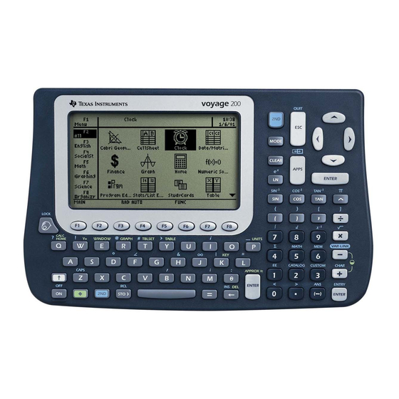
Page 6 Ê Ë Ì Ð Ï Í Î Voyage™ 200 Apps desktop Ê View full name of highlighted App. Ë ¸ Press to open highlighted App. Ì View time and date. Í Scroll down to view additional Apps. Î Check status line information. Ï...
Page 7 3. Lift the cover by the lip. To replace the cover, position it over the calculator with the lip in front and snap in place. Stowing the cover Stowing the cover Stowing the cover Stowing the cover To stow the cover, position it upside-down beneath the calculator with the lip in front and snap in place.
Page 8 Turning off the calculator Turning off the calculator Turning off the calculator Turning off the calculator Press 2 ®. The next time you turn on the calculator, the Apps desktop appears with the same settings and memory contents retained. (If you turned off the Apps desktop, the calculator Home screen appears.) You can use either of the following keys to turn off the Voyage™...
Page 9 Press: Description ¥ ® ¥ 2 ® (press Similar to except: ® and then press ¥ ® • You can use if an error message is displayed. • When you turn the Voyage™ 200 on again, it will be exactly as you left it. ®...
Page 10 Voyage™ 200 Voyage™ 200 keys Voyage™ 200 Voyage™ 200 keys keys keys Ë Ê Î Ì Í Voyage™ 200 keys Ê Function keys (ƒ– Š) open toolbar menus, access Apps, and edit categories of Apps. Getting Started...
Page 11 Ë Cursor keys (A, B, C, D) move the cursor. Ì Numeric keypad performs math and scientific functions. Í QWERTY keyboard is similar to a computer keyboard. Î Modifier keys (2, 8, 7 1) add features by increasing the number of key commands.
Page 12 2. Use the cursor keys to select a category. A submenu lists the characters in that category. 3. Use the cursor keys to select a character, and press ¸. Example: Enter the right arrow symbol ( ) in the Text Editor. Press Result Scroll down for...
Page 13 Press Result – or – Press repeatedly to select 9: Symbol displayed at cursor ¸ and press location. To open the keyboard map, press 8 ”. The keyboard map appears. To type most characters, press 8 and the corresponding key. Press N to close the map.
Page 14 Press Result Symbol displayed at cursor location. Modifier keys Modifier keys Modifier keys Modifier keys Modifier keys add features by increasing the number of keyboard operations at your fingertips. To access a modifier function, press a modifier key and then press the key for the corresponding operation.
Page 15 Keys Description Lets you use the cursor keys to manipulate geometric objects. Also used when drawing on a (Hand) graph. Example: Access the VAR-LINK [All] screen, where you can manage variables and Apps. Press Result 2 ° Function keys Function keys Function keys Function keys Use the function keys to perform the following operations:...
Page 16 Cursor keys Cursor keys Cursor keys Cursor keys Pressing A, B, C, or D moves the cursor in the corresponding direction. Depending on the App, and depending on whether the 2 orr8 modifier key is used, the cursor keys move the cursor in a variety of ways. C or D moves the cursor up or down one line at a time.
Page 17 Example: On the calculator Home screen, enter 0.00685 using scientific notation. Press Result ¶ ¸ Other important keys Other important keys Other important keys Other important keys Key Command Description Displays the Y= Editor. Displays the Window Editor. Displays the Graph screen. 8 &...
Page 18 Key Command Description These keys let you edit entered information by performing a cut, X (cut) copy, or paste operation. C (copy) V (paste) Displays the SAVE COPY AS dialog box, prompting you to select a folder and type a variable name to which data entered on the screen is saved.
Page 19 Key Command Description Deletes the character to the left of the cursor (backspace). Deletes the character to the right of the cursor. Switches between insert and overwrite modes. 2 ¯ Displays the MEMORY screen. Displays a list of commands. 2 £ Recalls the contents of a variable.
Page 20 Mode settings Mode settings Mode settings Mode settings Modes control how the Voyage™ 200 displays and interprets information. All numbers, including elements of matrices and lists, are displayed according to the current mode settings. When the Voyage™ 200 is turned off, the Constant Memory™ feature retains all of the mode settings you have selected.
Page 21 Press Result „ ã … Changing mode settings Changing mode settings Changing mode settings Changing mode settings Example: Change the Language mode setting to Spanish (Español). Press Result Getting Started...
Page 22 Press Result … Scroll down to the Language field. Press B and then press D until is highlighted. 3:Español Note: Your menu list might vary, depending on the languages installed. ¸ Getting Started...
Page 23 Press Result ¸ Note: The previous open App appears (in this example, the calculator Home screen). To return the Language mode setting to English, repeat the steps, selecting 1:English the Language field. Using the Catalog to access commands Using the Catalog to access commands Using the Catalog to access commands Using the Catalog to access commands Use the Catalog to access a list of Voyage™...
Page 24 Typing a letter takes you to the first command in the list starting with the same Note: letter. Press Result (displays Built-in commands) … (displays Flash Apps commands, if any) † (displays User-Defined commands, if any) Select commands from the Catalog and insert them onto the calculator Home screen entry line or paste them to other Apps, such as the Y= Editor, Text Editor, or CellSheet...
Page 25 Example: Insert the command on the calculator Home screen entry line. comDenom( Before selecting a command, position the cursor where you want the command to Note: appear. Pressing 2 D advances the Catalog list one page at a time. Press Result Then press until the pointer is...
Page 26 Selected command Command parameters Brackets [ ] indicate optional parameters To exit the Catalog without selecting a command, press N. Calculator Home screen Calculator Home screen Calculator Home screen Calculator Home screen The calculator Home screen is the starting point for math operations, including executing instructions, evaluating expressions, and viewing results.
Page 27 Ê Ë Ï Ì Î Í Ê History area lists the entry/answer pairs entered. Ë Tabs display menus for selecting lists of operations. Press ƒ, „, and so on to display menus. Ì Result of last entry is displayed here. (Note that results are not displayed on the entry line.) Í...
Page 28 About the history area About the history area About the history area About the history area The history area displays up to eight entry/answer pairs, depending on the complexity and height of the expressions. When the display is filled, information scrolls off the top of the screen.
Page 29 Interpreting history information on the status line Interpreting history information on the status line Interpreting history information on the status line Interpreting history information on the status line Use the history indicator on the status line for information about the entry/answer pairs. For example: If the cursor is on the entry line: Total number of pairs...
Page 30 • Enter on the calculator Home screen entry line. ClrHome To delete an entry/answer pair, move the cursor to either the entry or answer, and press 0 or M. Working with Apps Working with Apps Working with Apps Working with Apps The Voyage™...
Page 31 Option Description Creates a new file with the name typed in the field. Select an option, enter any required information, and press ¸. The App appears. Example: Create a new program using the Program Editor. Press Result Use cursor keys to highlight ¸...
Page 32 Press Result ¸ ¸ The newly created program variable, program1, is saved to the Main folder. Returning to the Apps desktop from within an App Returning to the Apps desktop from within an App Returning to the Apps desktop from within an App Returning to the Apps desktop from within an App Press O.
Page 33 The App icons for the selected category appear on the Apps desktop. Description „ All Icons for all installed Apps displayed. Not customizable. … English Customizable category. English is the default. † SocialSt Customizable category. SocialSt (social studies) is the default. ‡...
Page 34 Press ¸ or N to clear the message and return to the Apps desktop. Customizing the Apps Customizing the Apps categories Customizing the Apps Customizing the Apps categories categories categories The Voyage™ 200 organizes your Apps into seven categories, six of which you can customize to fit your individual needs.
Page 35 Example: Replace the Social Studies category with the Business category and add the CellSheet and Finance App shortcuts. Press Result ƒ – or – ¸ ¤ B u s i n e s s Getting Started...
Page 37 Open Apps and split-screen status Open Apps and split-screen status Open Apps and split-screen status Open Apps and split-screen status Your Voyage™ 200 lets you split the screen to view two Apps simultaneously. For example, view the Y= Editor and Graph screens simultaneously to see the list of functions and how they are graphed.
Page 38 Split-screen status (highlight indicates the portion where the Names of open Apps next App selected will open.) More information is available about using split screens. (For more information, see the electronic Split Screens chapter.) Checking status information Checking status information Checking status information Checking status information Look to the status line, located at the bottom of the screen, for information about the...
Page 39 Ê Ï Ë Ì Í Î Ð Ñ Ò Ó Indicator Meaning Ê Name of the selected folder (MAIN is the Current folder default folder.) Ë Modifier key Selected modifier key ( ), if any. Ì Hand key modifier key has been selected. Í...
Page 40 Indicator Meaning Ó BUSY–Calculation or graph is in progress Busy/Pause, PAUSE–You paused a graph or program Locked/Archived Œ variable –Variable opened in the current editor is locked or archived and cannot be modified Turning off the Apps desktop Turning off the Apps desktop Turning off the Apps desktop Turning off the Apps desktop You can turn off the Apps desktop from the MODE dialog box.
Page 41 Press Result D D B C ¸ ¸ Note: The previous open App appears (in this example, the calculator Home screen). To turn on the Apps desktop, repeat the procedure, selecting ON in the Apps Desktop mode field. To return to the Apps desktop from the calculator Home screen, press O. Using the clock Using the clock Using the clock...
Page 42 6 indicates you can scroll down for more options) Displaying the CLOCK dialog box Displaying the CLOCK dialog box Displaying the CLOCK dialog box Displaying the CLOCK dialog box 1. Use the cursor keys to highlight the Clock icon on the Apps desktop. 2.
Page 43 6. If the time format is 24 hours, proceed to step 9. — or — If the time format is 12 hours, press D to highlight the AM/PM field. 7. Press B to open the list of AM/PM options. 8. Press C or D to highlight an AM/PM option, then press ¸. The selected AM/PM option appears.
Page 44 9. Type the day, then press ¸ ¸ to save your settings and exit. The date is updated in the top right corner of the Apps desktop. Example: Set the time and date to 19/10/02 (October 19, 2002) at 1:30 p.m. Press Result Use cursor keys to highlight...
Page 45 Press Result 3 0 D ¸ Getting Started...
Page 46 Press Result ¸ 2 0 0 2 Scroll down to October ¸ and press Getting Started...
Page 47 Press Result D 1 9 ¸ ¸ Revised time and date Turning off the clock Turning off the clock Turning off the clock Turning off the clock From the Apps desktop, open the CLOCK dialog box and select OFF in the Clock field. Getting Started...
Page 48 Example: Turn off the clock. Press Result Use cursor keys to highlight Clock on ¸ Scroll down to the Clock field. ¸ Getting Started...
Page 49 Press Result ¸ Clock off To turn on the clock, repeat the procedure, selecting ON in the Clock field. Remember to reset the time and date. Using menus Using menus Using menus Using menus To select most Voyage™ 200 menus, press the function keys corresponding to the toolbars at the top of the calculator Home screen and most App screens.
Page 50 Other menus Other menus Other menus Other menus Use key commands to select the following menus. These menus contain the same options regardless of the screen displayed or the active App. Press To display CHAR menu. Lists characters not available on the keyboard;...
Page 51 Example: Select from the Algebra menu on the calculator Home screen. factor( Press Result Press: ¹ " – or – From the Apps desktop, use the cursor keys to highlight ¸ and press „ 6 indicates Algebra menu will open when you press „.
Page 52 Selecting submenu options Selecting submenu options Selecting submenu options Selecting submenu options A small arrow symbol (ú) to the right of a menu option indicates that selecting the option will open a submenu. $ points to additional options. Example: Select from the MATH menu on the calculator Home screen.
Page 53 Press Result – or – C C B – or – ¸ Using dialog boxes Using dialog boxes Using dialog boxes Using dialog boxes An ellipsis (…) at the end of a menu option indicates that choosing the option will open a dialog box.
Page 54 Example: Open the dialog box from the Window Editor. SAVE COPY AS Press Result Use the cursor keys to highlight and press ¸ ƒ Type the name of Press B to display – or – the variable. a list of folders. D ¸...
Page 55 Canceling a menu Canceling a menu Canceling a menu Canceling a menu To cancel a menu without making a selection, press N. Moving among toolbar menus Moving among toolbar menus Moving among toolbar menus Moving among toolbar menus To move among the toolbar menus without selecting a menu option: Press the function key (ƒ...
Page 56 Example: Turn on and turn off the custom menu from the calculator Home screen. Press Result Default custom menu Normal toolbar menu Example: Restore the default custom menu. Getting Started...
Page 57 Note: Restoring the default custom menu erases the previous custom menu. If you created the previous custom menu with a program, you can run the program again to reuse the menu. Press Result (to turn off the custom menu and turn on the standard toolbar menu) ˆ...
Page 58 Opening Apps with the Apps desktop turned off Opening Apps with the Apps desktop turned off Opening Apps with the Apps desktop turned off Opening Apps with the Apps desktop turned off If you turn off the Apps desktop, use the APPLICATIONS menu to open Apps. To open the APPLICATIONS menu with the Apps desktop off, press O.
Page 59 Using split screens Using split screens Using split screens Using split screens The Voyage™ 200 lets you split the screen to show two Apps at the same time. For example, display both the Y= Editor and Graph screens to compare the list of functions and how they are graphed.
Page 60 Press Result „ ¸ ¸ Getting Started...
Page 61 Setting the initial Apps for split screen Setting the initial Apps for split screen Setting the initial Apps for split screen Setting the initial Apps for split screen After you select either TOP-BOTTOM or LEFT-RIGHT split-screen mode, additional mode settings become available. Full-screen mode Split-screen mode Mode...
Page 62 Example: Display the Y= Editor in the top screen and the Graph App in the bottom screen. Press Result Getting Started...
Page 63 Press Result ¸ If you set Split 1 App and Split 2 App to the same nongraphing App or to the same graphing App with Number of Graphs set to 1, the Voyage™ 200 exits split-screen mode and displays the App in full-screen mode. Selecting the active App Selecting the active App Selecting the active App...
Page 64 A compatible graphing calculator. Adding Apps to your Voyage™ 200 is like loading software on a computer. All you need is TI Connect software and the the USB Silver Edition cable that came with your Voyage™ 200. For system requirements and instructions to link to compatible calculators and download TI Connect software, Apps, and OS versions, see the TI E&PS Web site.
Page 65 Finding the OS version and identification (ID) numbers Finding the OS version and identification (ID) numbers If you purchase software from the TI E&PS Web site or call the customer support number, you will be asked to provide information about your Voyage™ 200. You will find this information on the ABOUT screen.
Page 66 Note that your screen will be different than the one shown above. Deleting an Application Deleting an Application Deleting an Application Deleting an Application Deleting an application removes it from the Voyage™ 200 and increases space for other applications. Before deleting an application, consider storing it on a computer for reinstallation later.
Page 67 Voyage™ 200 to a compatible graphing calculator or peripheral device, such as a TI-89 or TI-92 Plus graphing calculator or the CBL 2™ and CBR™ systems. To show your calculator’s display to the classroom – Use the accessory port to connect the TI-Presenter™...
Page 68 Important OS download information Important OS download information Important OS download information Important OS download information New batteries should be installed before beginning an OS download. When in OS download mode, the APD feature does not function. If you leave your calculator in download mode for an extended time before you actually start the download, your batteries may become depleted.
Page 69 Installing the AAA Batteries Installing the AAA Batteries Installing the AAA Batteries Installing the AAA Batteries 1. Remove the battery cover from the back of the calculator. 2. Unwrap the four AAA batteries provided with your product and insert them in the battery compartment.
Page 70 Previews Previews Previews Previews Performing Computations Performing Computations Performing Computations Performing Computations This section provides several examples for you to perform from the Calculator Home screen that demonstrate some of the computational features of the Voyage™ 200. The history area in each screen was cleared by pressing ƒ and selecting 8:Clear Home before performing each example, to illustrate only the results of the example’s keystrokes.
Page 71 Finding the Factorial of Numbers Finding the Factorial of Numbers Finding the Factorial of Numbers Finding the Factorial of Numbers Steps and keystrokes Display Compute the factorial of several numbers to see how the Voyage™ 200 handles very large integers. To get the factorial operator (!), press 2 I, select , and then 7:Probability...
Page 72 Finding Prime Factors Finding Prime Factors Finding Prime Factors Finding Prime Factors Steps and keystrokes Display Compute the factors of the rational number 2634492. You can enter “factor” on the entry line by typing on the keyboard, or by FACTOR pressing „...
Page 73 Expanding Expressions Expanding Expressions Expanding Expressions Expanding Expressions Steps and keystrokes Display Expand the expression (xN5) . You can enter “expand” on the entry line by typing EXPAND on the keyboard, or by pressing „ and selecting 3:expand( Press „ 3 c X | 5 d Z 3 d ¸ (Optional) Enter other expressions on your own.
Page 74 Factoring Polynomials Factoring Polynomials Factoring Polynomials Factoring Polynomials Steps and keystrokes Display Factor the polynomial (x N5) with respect to x. You can enter “factor” on the entry line by typing on the keyboard or by pressing FACTOR „ and selecting 2:factor( Press „...
Page 75 Solving Equations with a Domain Constraint Solving Equations with a Domain Constraint Solving Equations with a Domain Constraint Solving Equations with a Domain Constraint Steps and keystrokes Display Solve the equation x N2xN6=2 with respect to x where x is greater than zero. The “with” (I) operator provides domain constraint.
Page 76 Finding the Derivative of Functions Finding the Derivative of Functions Finding the Derivative of Functions Finding the Derivative of Functions Steps and keystrokes Display Find the derivative of (xNy) /(x+y) with respect to x. This example illustrates using the calculus differentiation function and how the function is displayed in “pretty print”...
Page 77 Finding the Integral of Functions Steps and keystrokes Display Find the integral of with respect to x. …s in(x) This example illustrates using the calculus integration function. Press 2 < X p W X d b X d ¸ Solving Problems Involving Vectors Steps and keystrokes Display 1.
Page 78 Log to Any Base Steps and keystrokes Display Find log (x,b). You can enter “log” on the entry line by typing on the keyboard, or by pressing 8 7. Press 8 7 X , b d ¸ Converting Angle Measures Converting Angle Measures Converting Angle Measures Converting Angle Measures...
Page 79 Steps and keystrokes Display 2. Convert 345 degrees to Radian angle measure. ú You can enter “ Rad ” on the entry line ú by selecting “ Rad ” from the Catalog menu, or from the Math menu by pressing 2 I and selecting 2:angle, B:úRad Note: You can also use ó,ô, or...
Page 80 equation, and solve for the value of y. Then substitute the y value back into the first equation to solve for the value of x. Steps and keystrokes Display 1. Display the Home screen and clear the entry line. Solve the equation 2x N 3y = 4 for x.
Page 81 Steps and keystrokes Display 4. Highlight the equation for x in the history area. Press C C C 5. Auto-paste the highlighted expression to the entry line. Then substitute the value of y that was calculated from the second equation. Press ¸...
Page 82 acceleration due to gravity, which is a constant named _g). Convert the result from newtons to kilograms of force. Steps and keystrokes Display 1. Display the dialog box, Page 3. For MODE mode, select for the metric Unit System system of measurements. Results are displayed according to these default units.
Page 83 Steps and keystrokes Display 2. Create an acceleration unit for meters/second named _ms2. dialog box lets you select units UNITS from an alphabetical list of categories. You can use 2 D and 2 C to scroll one page at a time through the categories.
Page 84 Steps and keystrokes Display 3. Calculate the force when m = 5 kilograms (_kg) and a = 20 meters/second (_ms2). If you know the abbreviation for a unit, you can type it from the keyboard. Press 5 2 5 KG p 20 2 5 MS2 ¸...
Page 85 Basic Function Graphing I Basic Function Graphing I Basic Function Graphing I Basic Function Graphing I The example in this section demonstrates some of the graphing capabilities of the Voyage™ 200 keystrokes. It illustrates how to graph a function using the .
Page 86 Steps and keystrokes Display 3. Display the graph of the function. Select by pressing or by 6:ZoomStd moving the cursor to 6:ZoomStd pressing ¸. Press „ 6 4. Turn on Trace The tracing cursor, and the x and y coordinates are displayed. Press …...
Page 87 Steps and keystrokes Display 7. Set the upper bound. Press B (right cursor) to move the tracing cursor until the upper bound for x is just to the right of the minimum node. Press B ... B 8. Find the minimum point on the graph between the lower and upper bounds.
Page 88 Basic Function Graphing II Basic Function Graphing II Basic Function Graphing II Basic Function Graphing II Graph a circle of radius 5, centered on the origin of the coordinate system. View the circle using the standard viewing window ( ). Then use to adjust the ZoomStd ZoomSqr...
Page 89 Steps and keystrokes Display 4. Define y2(x) = – – , the function for the bottom half of the circle. The bottom half is the negative of the top half, so you can define y2(x) = Ly1(x). Use the full function name , not y1(x) simply y1.
Page 90 Depending on the viewing window, however, the plotted endpoints for each half may be slightly different from their mathematical endpoints. Basic Function Graphing III Basic Function Graphing III Basic Function Graphing III Basic Function Graphing III Use the “Detect Discontinuities” graph format to eliminate faux asymptotes and connections in a jump discontinuity.
Page 91 Steps and keystrokes Display 4. Execute the command, which Graph automatically displays the Graph screen. Observe the “faux” asymptotes contained in the graph. Press 8 %q 5. Display the Graph Formats dialog box and set “Detect Discontinuities” to ON. Note: The second item on the Graph Format dialog is greyed out, which means the graph order is set to sequential “Seq”.
Page 92 Parametric Graphing Parametric Graphing Parametric Graphing Parametric Graphing Graph the parametric equations describing the path of a ball kicked at an angle (q) of 60¡ with an initial velocity (v ) of 15 meters/sec. The gravity constant g = 9.8 meters/sec Ignoring air resistance and other drag forces, what is the maximum height of the ball and when does it hit the ground? Steps and keystrokes...
Page 93 Steps and keystrokes Display 3. Define the vertical component yt1(t) = v t sin q N (g/2)t Enter values for v , q, and g. Press ¸ 15T p W 60 2 “ d | c 9.8 e 2 d T Z 2 ¸ 4.
Page 94 Polar Graphing Polar Graphing Polar Graphing Polar Graphing The graph of the polar equation r1(q) = A sin forms the shape of a rose. Graph the rose for A=8 and B=2.5. Then explore the appearance of the rose for other values of A and B.
Page 95 Steps and keystrokes Display 3. Select the viewing window, ZoomStd which graphs the equation. • The graph shows only five rose petals. In the standard viewing window, the Window variable qmax = 2p. The remaining petals have q values greater than 2p. •...
Page 96 Steps and keystrokes Display 5. Select , which regraphs the ZoomSqr equation. increases the range along the ZoomSqr x axis so that the graph is shown in correct proportion. Press „ 5 You can change values for A and B as necessary and regraph the equation.
Page 97 Steps and keystrokes Display 1. Display the dialog box. For MODE Graph mode, select SEQUENCE Press 3 B 4 ¸ 2. Display and clear the . Then Y= Editor define the sequence as u1(n) = iPart(.8…u1(nN1)+1000). to take the integer part of the iPart result.
Page 98 Steps and keystrokes Display 5. Set the x and y Window variables to appropriate values for this example. Press 0 D 50 D 10 D 0 D 6000 D 1000 6. Display the Graph screen. Press 8 % 7. Select .
Page 99 3D Graphing 3D Graphing 3D Graphing 3D Graphing Graph the 3D equation z(x,y) = (x y N y x) / 390. Animate the graph by using the cursor to interactively change the eye Window variable values that control your viewing angle. Then view the graph in different graph format styles.
Page 100 Steps and keystrokes Display 4. Select the viewing cube, which ZoomStd automatically graphs the equation. As the equation is evaluated (before it is graphed), “evaluation percentages” are shown in the upper-left part of the screen. Press „ 6 Note: If you have already used 3D graphing, the graph may be shown in expanded view.
Page 101 Steps and keystrokes Display 6. Return the graph to its initial orientation. Then move the viewing angle along the “viewing orbit” around the graph. Press 0 (zero, not the letter O) A A A 7. View the graph along the x axis, the y axis, and then the z axis.
Page 102 Steps and keystrokes Display 9. Display the graph in different graph format styles. Press F (press F to switch from each style to the next) HIDDEN SURFACE CONTOUR LEVELS (may require extra time to calculate contours) WIRE AND CONTOUR WIRE FRAME Previews...
Page 103 Note: You can also display the graph as an implicit plot by using the GRAPH FORMATS dialog box ( 8 F). If you press F to switch between styles, the implicit plot is not displayed. Differential Equation Graphing Differential Equation Graphing Differential Equation Graphing Differential Equation Graphing Graph the solution to the logistic 1st-order differential equation y' = .001y…(100Ny).
Page 104 Steps and keystrokes Display 2. Display and clear the . Then Y= Editor define the 1st-order differential equation: y1'(t)=.001y1…(100Ny1) Press p to enter the … shown above. Do not use implied multiplication between the variable and parentheses. If you do, it is treated as a function call.
Page 105 Steps and keystrokes Display 4. Display the , and set the Window Editor Window variables as shown to the right. Press 8 $ 0 D 10 D .1 D 0 D ? 10 D 110 D 10 D ? 10 D 120 D 10 D 0 D .001 D 20 5.
Page 106 Steps and keystrokes Display 8. Return to the and change Y= Editor enter two initial conditions as a list: yi1={10,20} Press 8 # C ¸ 2 [ 10 b 20 2 \ ¸ 9. Return to the Graph screen. Press 8 % Previews...
Page 107 Steps and keystrokes Display 10. To select an initial condition interactively, press: Š When prompted, enter t=40 and y1=45. When selecting an initial condition interactively, you can specify a value for t other than the t value entered in the Y= Editor Window Editor Instead of entering...
Page 108 Additional Graphing Topics Additional Graphing Topics Additional Graphing Topics Additional Graphing Topics From the Home screen, graph the piecewise defined function: y = Lx when x < 0 and y = 5 cos(x) when x ‚ 0. Draw a horizontal line across the top of the cosine curve. Then save a picture of the displayed graph.
Page 109 Steps and keystrokes Display 4. Draw a horizontal line across the top of the cosine curve. The calculator remains in “horizontal” mode until you select a different operation or press N. Press ‰ 5 C (until the line is positioned) ¸...
Page 110 Steps and keystrokes Display 7. Open the saved picture variable to redisplay the graph with the line. Be sure to set . By default, it Type = Picture is set to Press , 1 B 2 (if not already shown, also set Variable = pic1) ¸...
Page 111 Steps and keystrokes Display 2. Display and clear the . Then Y= Editor define y1(x) = x N 2x. Press 8 # , 8 ¸ ¸ X Z 3 | 2 X ¸ 3. Set the table parameters to: tblStart = tbl = 1 Graph <...
Page 112 Steps and keystrokes Display 6. Zoom in on the sign change between x = L2 and x = L1 by changing the table parameters to: tblStart = L2 @tbl = .1 Press „ ? 2 D .1 ¸ ¸ Split Screens Split Screens Split Screens Split Screens...
Page 113 Steps and keystrokes Display 2. Clear the and turn off any stat Y= Editor data plots. Define y1(x) = .1x N2x+6. A thick border around the Y= Editor indicates it is active. When active, its entry line goes all the way across the display.
Page 114 Steps and keystrokes Display 5. Switch to the Graph screen, which regraphs the edited function. The thick border is around the Graph screen. Press 2 a 6. Switch to the and open the Y= Editor in its place. Window Editor Press 2 a 8 $ 7.
Page 115 Data/Matrix Editor Data/Matrix Editor Data/Matrix Editor Data/Matrix Editor Use the to create a one-column list variable. Then add a second Data/Matrix Editor column of information. Notice that the list variable (which can have only one column) is automatically converted into a data variable (which can have multiple columns). Steps and keystrokes Display 1.
Page 116 Steps and keystrokes Display 3. Move to column 2, and define its column header so that it is twice the value of column 1. DATA is shown in the upper-left corner to indicate that the list variable was Œ means the cell is in converted to a data variable.
Page 117 Statistics and Data Plots Statistics and Data Plots Statistics and Data Plots Statistics and Data Plots Based on a sample of seven cities, enter data that relates population to the number of buildings with more than 12 stories. Using Median-Median and linear regression calculations, find and plot equations to fit the data.
Page 118 Steps and keystrokes Display 3. Using the sample data below, enter the population in column 1. Pop. (in 1000s) Bldgs > 12 stories Press 150 ¸ 500 ¸ 800 ¸ 250 ¸ 500 ¸ 750 ¸ 950 ¸ 4. Move the cursor to row 1 in column 2 (r1c2).
Page 119 Steps and keystrokes Display 5. Move the cursor to row 1 in column 1 (r1c1). Sort the data in ascending order of population. This sorts column 1 and then adjusts all other columns so that they retain the same order as column 1. This is critical for maintaining the relationships between columns of data.
Page 120 Steps and keystrokes Display 7. Perform the calculation to display the MedMed regression equation. As specified on the dialog box, Calculate this equation is stored in y1(x). Press ¸ 8. Close the screen. The STAT VARS displays. Data/Matrix Editor Press ¸ 9.
Page 121 Steps and keystrokes Display 12. Display the Plot Setup screen. is highlighted by default. Plot 1 … lets you clear highlighted Plot settings. Press „ 13. Define Plot 1 Plot Type = Scatter Mark = Box x = C1 y = C2 Notice the similarities between this and dialog box.
Page 122 Steps and keystrokes Display 15. Display the . For , the Y= Editor y1(x) MedMed regression equation, set the display style to Note: Depending on the previous contents of your , you may need Y= Editor to move the cursor to y1. at the top of the screen means PLOTS 1 that...
Page 123 Steps and keystrokes Display 18. Return to the current session of the Data/Matrix Editor Press O D ¸ ¸ 19. Enter a title for column 3. Define column 3’s header as the values predicted by the MedMed line. To enter a title, the cursor must highlight the title cell at the very top of the column.
Page 124 Steps and keystrokes Display 21. Enter a title for column 5. Define column 5’s header as the values predicted by the LinReg line. Press B C LIN ¸ † Y2 c C1 d ¸ 22. Enter a title for column 6. Define column 6’s header as the residuals for LinReg.
Page 125 Steps and keystrokes Display 25. Highlight and define it as: Plot 3 Plot Type = Scatter Mark = Plus x = C1 (LinReg residuals) y = C6 Press D , D B 3 D C1 D C6 ¸ ¸ and turn all the 26.
Page 126 Steps and keystrokes Display 29. Use the MedMed ( ) and y1(x) LinReg ( ) regression equations to y2(x) calculate values for x = 300 (300,000 population). function ( 2 I 1 3) round ensures that results show an integer number of buildings.
Page 127 Steps and keystrokes Display 2. Type PROG1 (with no spaces) as the name of the new program variable. Press D D PROG 1 3. Display the “template” for a new program. The program name, Prgm, and EndPrgm are shown automatically. After typing in an input box such as Variable, you must press ¸...
Page 128 Steps and keystrokes Display 4. Type the following program lines. Request "Enter an integer",n Displays a dialog box that prompts “Enter an integer”, waits for the user to enter a value, and stores it (as a string) to variable n. expr(n) Converts the string to a numeric expression.
Page 129 Steps and keystrokes Display 5. Go to the Home screen. Enter the prog1() program name, followed by a set of parentheses. You must include ( ) even when there are no arguments for the program. The program displays a dialog box with the prompt specified in the program.
Page 130 Steps and keystrokes Display 8. Leave the Program I/O screen and return to the Home screen. You can also press N, 2 K, or 8 " to return to the Home screen. Press ‡ Text Operations Text Operations Text Operations Text Operations Start a new session.
Page 131 Steps and keystrokes Display 3. Type some sample text. • To type a single uppercase letter, press 7 and then the letter. Practice editing your text by using: • The cursor pad to move the text cursor. 0 or 8 . to delete the character •...
Page 132 Numeric Solver Numeric Solver Numeric Solver Numeric Solver Consider the equation a=(m2Nm1)/(m2+m1)…g, where the known values are m2=10 and g=9.8. If you assume that a=1/3 g, find the value of m1. Steps and keystrokes Display 1. Use Oto display the Numeric Solver 2.
Page 133 Steps and keystrokes Display 4. Move the cursor to the unknown variable Optionally, you can enter an initial guess for m1. Even if you enter a value for all variables, the Numeric Solver solves for the variable marked by the cursor. g/3 is evaluated when Press D D you move the cursor...
Page 134 Steps and keystrokes Display 7. Return to the and exit the Numeric Solver split screen. You can press ¸ or D to redisplay the list of variables. Press 2 a … 2 Number Bases Number Bases Number Bases Number Bases Calculate 10 binary (base 2) + F hexadecimal (base 16) + 10 decimal (base 10).
Page 135 Steps and keystrokes Display 2. Calculate 0b10+0hF+10. To enter a binary or hex number, you must use the 0b or 0h prefix (zero and the letter B or H). Otherwise, the entry is treated as a decimal number. Note: The 0b or 0h prefix is a zero, not the letter O, followed by B or H.
Page 136 Steps and keystrokes Display 6. Change the mode to Base When , the magnitude of Base = HEX a result is restricted to certain size limitations. Press 3 „ (use D to move to Base mode) B 2 ¸ 7. Calculate 0b10+0hF+10. Press 0 B 10 «...
Page 137 variables are locked automatically.) Finally, unarchive the variable and delete the unused variables so that they will not take up memory. Steps and keystrokes Display 1. From the Home screen, assign variables with the following variable types. Expression: 5 !x1 +4 !f(x) Function: {5,10} !L1...
Page 138 Steps and keystrokes Display 4. Change the screen’s view to show only function variables. Although this may not seem particularly useful in an example with four variables, consider how useful it could be if there were many variables of all different types. Press „...
Page 139 Steps and keystrokes Display 8. Complete the operation. 5…f(2) Press 2 d ¸ Previews...
Page 140 Archiving a variable Archiving a variable Archiving a variable Archiving a variable Steps and keystrokes Display 1. Redisplay , and highlight the VAR-LINK variable you want to archive. The previous change in view is no longer in effect. The screen lists all defined variables.
Page 141 Steps and keystrokes Display 4. Attempt to store a different value to the archived variable. Press 10 9 X1 ¸ 5. Cancel the error message. Press N 6. Use to unarchive the variable. VAR-LINK Press 2 ° (use D to highlight ) , 9 7.
Page 142 Deleting variables Deleting variables Deleting variables Deleting variables Steps and keystrokes Display , and use the ‡ 1. Display VAR-LINK toolbar menu to select all variables. A Ÿ mark indicates items that are selected. Notice that this also selected the MAIN folder. Note: Instead of using ‡...
Page 143 Steps and keystrokes Display 4. Because ‡ also selected the MAIN folder, an error message states that you cannot delete the MAIN folder. Acknowledge the message. When is redisplayed, the VAR-LINK deleted variables are not listed. Press ¸ 5. Close and return to the current VAR-LINK application (Home screen in this...
Page 144 Operating the Calculator Operating the Calculator Operating the Calculator Operating the Calculator Turning the Calculator On and Off Turning the Calculator On and Off Turning the Calculator On and Off Turning the Calculator On and Off You can turn your graphing calculator on and off manually by using the ´ and 2 ® (or 8 ®) keys.
Page 145 Turning the Calculator Off Turning the Calculator Off Turning the Calculator Off Turning the Calculator Off You can use either of the following keys to turn off your graphing calculator. Press: Description 2 ® Settings and memory contents are retained by the Constant Memory™...
Page 146 APD does not occur if a calculation or program is in progress, unless the program is paused. If a program is running, but waiting for a key press, APD will occur after several minutes of inactivity. Setting the Display Contrast Setting the Display Contrast Setting the Display Contrast Setting the Display Contrast...
Page 147 When to Replace Batteries When to Replace Batteries When to Replace Batteries When to Replace Batteries As the batteries get low, the display begins to dim (especially during calculations) and you must increase the contrast. If you have to increase the contrast frequently, replace the four alkaline batteries.
Page 148 Í Ê Î Ë Ì Ê ƒ Š – open toolbar menus. Ë QWERTY keyboard functions the same as a computer keyboard. Ì 8 ¤ ‚ add functionality by increasing the available key commands. Í A , and move the cursor. Î...
Page 149 C and A, C and B, D and A, or D and B to move diagonally. (Press the indicated • cursor keys simultaneously.) Modifier Keys Modifier Keys Modifier Keys Modifier Keys Modifier Keys Modifier Keys Modifier Keys Modifier Keys Modifier Description Accesses the second function of the next key you press.
Page 150 The following Voyage™ 200 Graphing Calculator example shows using the 2 or 8 modifier key with the Y alphabetic key. 2  TABLE accesses displays the (convert). The convert Table screen. The word is symbol is the same color the same color as the as the key.
Page 151 Description These keys let you edit entered information by performing a cut, copy, or paste operation. X (cut) C (copy) V (paste) Toggles between the last two chosen Apps or between split screen portions. 2 ¾ Toggles the custom menu on and off. 2 ...
Page 152 Description 2 £ Recalls the contents of a variable. H 8 À Displays the UNITS dialog box. 2 ¿ Displays the CHAR menu, which lets you select Greek letters, international accented characters, etc. Recalls the previous entry and the last answer, 2 ±...
Page 153 Press: 2 ¢ Turn on uppercase ALPHA-lock. 2 ¢ Turn off alpha-lock. (turns off uppercase lock) For Special Characters For Special Characters For Special Characters For Special Characters Use the 2 ¿ menu to select from a variety of special characters. For more information, refer to “Entering Special Characters”...
Page 154 module. For example, it is important to know that functions such as x are evaluated before negation. Use c and d to include parentheses if you Evaluated as have any doubt about how a negation will be evaluated. If you use | instead of · (or vice versa), you may get an error message or you may get unexpected results.
Page 155 2. Press: í appears in the display. 3. Type the exponent as an integer with up to 3 digits. You can use a negative exponent. Entering a number in scientific notation does not cause the answers to be displayed in scientific or engineering notation.
Page 156 Definitions Definitions Definitions Definitions Expression Consists of numbers, variables, operators, functions, and their arguments that evaluate to a single answer. For example: • Enter an expression in the same order that it normally is written. • In most places where you are required to enter a value, you can enter an expression.
Page 157 • This guidebook uses the word command as a generic reference to both functions and instructions. Implied Multiplication Implied Multiplication Implied Multiplication Implied Multiplication The graphing calculator recognizes implied multiplication, provided it does not conflict with a reserved notation. If you enter: The calculator interprets it as: ùp Valid...
Page 158 Entering an Expression Entering an Expression Entering an Expression Entering an Expression Type the expression, and then press ¸ to evaluate it. To enter a function or instruction name on the entry line, you can: • Press its key, if available. For example, press:W –...
Page 159 Voyage™ 200 Press Display 3.76 3.76/( 7.9+ ‡ c · « 2 ] inserts ‡( because its argument must be in parentheses. 3.76/( 7.9+ ‡ (5)) once to close ‡ (5) and again to close ( 7.9 + ‡ « 3.76/( 7.9+ (5))+2log(45)
Page 160 Entering Multiple Expressions on a Line Entering Multiple Expressions on a Line Entering Multiple Expressions on a Line Entering Multiple Expressions on a Line Ê To enter more than one expression or instruction at a time, separate them with a colon by pressing 2 Ë.
Page 161 2. As necessary, use C and D to highlight the entry or answer you want to view. For example, C moves from answer to entry, up through the history area. 3. Use B and A or 2 B and 2 A to scroll right and left.
Page 162 Voyage™ 200 Press Display e c · « 3.76 ¸ « 2 LOG « When you press , the ¸ entry line is replaced with the variable ans(1), which contains the last answer. Stopping a Calculation Stopping a Calculation Stopping a Calculation Stopping a Calculation When a calculation is in progress, BUSY appears on the right end of the status line.
Page 163 Pretty Print Mode Pretty Print Mode Pretty Print Mode Pretty Print Mode By default, . Exponents, roots, fractions, etc., are displayed in the same Pretty Print = ON form in which they are traditionally written. You can use 3 to turn pretty print off and Pretty Print –...
Page 164 — Any result that is not a whole number is displayed in a fractional or symbolic EXACT form (1/2, p, , etc.). Shows whole-number results. Shows simplified fractional results. Shows symbolic Shows symbolic form of roots that cannot be evaluated to a whole number. 8 ¸...
Page 165 — All numeric results, where possible, are displayed in floating-point APPROXIMATE (decimal) form. Results are rounded to the precision of your graphing calculator and displayed Note: according to current mode settings. Fractional results are evaluated numerically. Symbolic forms, where possible, are evaluated numerically Because undefined variables cannot be evaluated, they are treated algebraically.
Page 166 To retain an EXACT form, use fractions instead of decimals. For example, use 3/2 Note: instead of 1.5. The following chart compares the three settings. Exact Approximate Auto Entry Result Result Result 1.33333 ù 51/2 25.5 25.5 — A decimal in the entry forces a .707107 (2)/2...
Page 167 Internally, the calculator calculates and retains all decimal results with up to 14 significant digits (although a maximum of 12 are displayed). Setting Example Description 123. (FIX 0) Results are rounded to the (0–12) 123.5 (FIX 1) selected number of decimal 123.46 (FIX 2) places.
Page 168: Editing An Expression In The Entry Line
Setting Example Description NORMAL 12345.6 If a result cannot be displayed in the number of digits specified by the calculator Display Digits mode, the switches from NORMAL to SCIENTIFIC for that result only. SCIENTIFIC 1.23456E 4 1.23456 Ê Ë ENGINEERING 1.23456E 3 12.3456 Ì...
Page 169 Removing the Highlight from the Previous Entry Removing the Highlight from the Previous Entry Removing the Highlight from the Previous Entry Removing the Highlight from the Previous Entry After you press ¸ to evaluate an expression, the calculator leaves that expression on the entry line and highlights it.
Page 170 Deleting a Character Deleting a Character Deleting a Character Deleting a Character To delete: Press: The character to the left of Hold to delete multiple the cursor. characters. The character to the right of the cursor. All characters to the right of If there are no characters to the cursor.
Page 171 Inserting or Overtyping a Character Inserting or Overtyping a Character Inserting or Overtyping a Character Inserting or Overtyping a Character The calculator has both an insert and an overtype mode. By default, the calculator is in the insert mode. To toggle between the insert and overtype modes, press 2 /. If in: The next character you type:...
Page 172 To highlight multiple characters: 1. Move the cursor to either side of the characters you want to highlight. To replace sin( with cos(, place the cursor beside sin. 2. Hold ¤ and press A or B to highlight characters left or right of the cursor. ¤...
Page 173 are described in the appropriate modules. Displaying a Menu Displaying a Menu Displaying a Menu Displaying a Menu Press: To display: ƒ „ A toolbar menu — Drops down from the toolbar at the , etc. top of most application screens. Lets you select operations useful for that application.
Page 174 Selecting an Item from a Menu Selecting an Item from a Menu Selecting an Item from a Menu Selecting an Item from a Menu To select an item from the displayed menu, either: • Press the number or letter shown to the left of that item. –...
Page 175 For example, List displays a submenu that lets you select a specific List function. indicates that you can use the cursor pad to scroll down for additional items. For items that have a submenu, you can use the cursor pad as described below. To display the submenu for the highlighted item, press B.
Page 176 For example, Save Copy As ... displays a dialog box that prompts you to select a folder name and type a variable name. indicates that you can press " display and select from a menu. An input box indicates that you must type a value.
Page 177 When using B, be sure that an item with a submenu is not highlighted. If so, B displays that item’s submenu instead of moving to the next toolbar menu. Example: Selecting a Menu Item Example: Selecting a Menu Item Example: Selecting a Menu Item Example: Selecting a Menu Item Round the value of p to three decimal places.
Page 178 From the APPLICATIONS Menu From the APPLICATIONS Menu From the APPLICATIONS Menu From the APPLICATIONS Menu 1. If the Apps desktop is off, press O to display a menu that lists the applications. To cancel the menu without making a selection, press N. Note: 2.
Page 179 Application: Lets you: Numeric Solver Enter an expression or equation, define values for all but one variable, and then solve for the unknown variable. Home Enter expressions and instructions, and perform calculations. From the Apps Desktop From the Apps Desktop From the Apps Desktop From the Apps Desktop Press the first letter of the application name, or use the cursor keys to highlight an...
Page 180 Option Description Creates a new file with the name typed in the field. Select an option and press ¸. The application appears. The general term variable is used to refer to the application data files that you Note: create. Use any of these methods to return to the Apps desktop from within an application: Press O.
Page 181 From the Keyboard From the Keyboard From the Keyboard From the Keyboard Operating the Calculator...
Page 182 You can access commonly used applications from the keyboard. This guidebook uses the notation 8 #, similar to the notation used in second functions. Application: Press: Home " " Applications listed ƒ „ above etc., Y= Editor are printed in the Window Editor same color as Graph...
Page 183 Setting Modes Setting Modes Setting Modes Setting Modes Modes control how numbers and graphs are displayed and interpreted. Mode settings are retained by the Constant Memory™ feature when the graphing calculator is turned off. All numbers, including elements of matrices and lists, are displayed according to the current mode settings.
Page 184 Changing Mode Settings Changing Mode Settings Changing Mode Settings Changing Mode Settings From the MODE dialog box: 1. Highlight the mode setting you want to change. Use D or C (with ƒ, „, or …) to scroll through the list. 2.
Page 185 Overview of the Modes Overview of the Modes Overview of the Modes Overview of the Modes For detailed information about a particular mode, look in the applicable section of Note: this guidebook. Mode Description Graph Type of graphs to plot: FUNCTION, PARAMETRIC, POLAR, SEQUENCE, 3D, or DE.
Page 186 Mode Description Split Screen Splits the screen into two parts and specifies how the parts are arranged: FULL (no split screen), TOP-BOTTOM, or LEFT-RIGHT. Refer to the Split Screens module. Split 1 App Application in the top or left side of a split screen. If you are not using a split screen, this is the current application.
Page 187 Mode Description Language Lets you localize the calculator into one of several languages, depending on which language Flash applications are installed. Apps Desktop Turns the Apps desktop ON or OFF. Using the Clean Up Menu to Start a New Problem Using the Clean Up Menu to Start a New Problem Using the Clean Up Menu to Start a New Problem Using the Clean Up Menu to Start a New Problem...
Page 188 Menu Item Description Single-character variable names are often used in symbolic calculations such as: solve(a ¦ ¦ x+c=0,x) If any of the variables have already been assigned a value, your calculation may produce misleading results. To prevent this, you can select 1:Clear a–z before beginning the calculation.
Page 189 Using the Catalog Dialog Box Using the Catalog Dialog Box Using the Catalog Dialog Box Using the Catalog Dialog Box The CATALOG provides a way to access any built-in command (functions and instructions) from one convenient list. In addition, the CATALOG dialog box lets you select functions used in Flash applications or user-defined functions (if any have been loaded or defined).
Page 190 Options that are not currently valid are dimmed. For example, … Note: Flash Apps dimmed if you have not installed a Flash application. † is dimmed if you User-Defined have not created a function or a program. Selecting a Built-in Command from the CATALOG Selecting a Built-in Command from the CATALOG Selecting a Built-in Command from the CATALOG Selecting a Built-in Command from the CATALOG...
Page 191 Press or type: To move the indicator: To the first function that The letter key. begins with a specified letter From the top of the list, press C to move to the bottom. From the bottom, press D Note: to move to the top. Information about Parameters Information about Parameters Information about Parameters...
Page 192 For details about the parameters, refer to that command’s description in the Note: Technical Reference module. Viewing CATALOG Help Viewing CATALOG Help Viewing CATALOG Help Viewing CATALOG Help You can display a command's parameters in a dialog box by pressing ƒ .
Page 193 2. Press … . (This option is dimmed if no Flash applications are installed.) Flash Apps • The list is alphabetized by function name. The left column lists functions. The right column lists the Flash application that contains the function. •...
Page 194 When you select a function or program, its name is inserted in the entry line at the cursor location. Therefore, you should position the cursor as necessary before selecting the function or program. 1. Press: 2 ½ 2. Press † .
Page 195 Storing and Recalling Variable Values Storing and Recalling Variable Values Storing and Recalling Variable Values Storing and Recalling Variable Values When you store a value, you store it as a named variable. You can then use the name instead of the value in expressions. When the calculator encounters the name in an expression, it substitutes the variable’s stored value.
Page 196 Examples Examples Examples Examples Variable Description myvar Not OK, name is preassigned to the log function. Log1 3rdTotal Not OK, starts with a digit. circumfer Not OK, more than 8 characters. Data Types Data Types Data Types Data Types DataTypes Examples Expressions 2.54, 1.25E6, 2...
Page 197 1. Enter the value you want to store, which can be an expression. 2. Press §. The store symbol (!) is displayed. 3. Type the variable name. TI-89 Titanium users should use Note: j as necessary when typing variable names.
Page 198 Using a Variable in an Expression Using a Variable in an Expression Using a Variable in an Expression Using a Variable in an Expression 1. Type the variable name into the expression. 2. Press ¸ to evaluate the expression. The variable’s value To view a list of existing variable Note: did not change.
Page 199 Status Line Indicators in the Display Status Line Indicators in the Display Status Line Indicators in the Display Status Line Indicators in the Display The status line is displayed at the bottom of all application screens. It shows information about the current state of the calculator, including several important mode settings. Status Line Indicators Status Line Indicators Status Line Indicators...
Page 200 Indicator Meaning — will use the diamond feature of the next key you press. ¤ — will type the uppercase letter for the next key you press. When used in combination with a cursor key, the Voyage™ 200 will use any “dragging” features that are available in graphing and geometry.
Page 201 Indicator Meaning x(t) and y(t) parametric equations ) polar equations u(n) sequences z(x,y) 3D equations y'(t) differential equations Battery Displayed only when the batteries are getting low. If BATT is shown with a black background, change the batteries as soon as possible. History Pairs, The information shown in this part of the status line Busy/Pause,...
Page 202 • If the next key you press does not have a diamond feature or an associated letter, the key performs its normal operation. Operating the Calculator...
Page 203 Calculator Home Screen Calculator Home Screen Calculator Home Screen Calculator Home Screen Calculator Home Screen Calculator Home Screen Calculator Home Screen Calculator Home Screen The calculator Home screen is the starting point for math operations, including executing instructions, evaluating expressions, and viewing results. A blank calculator Home screen This module describes the parts of the calculator Home screen, how to scroll through or modify the history area;...
Page 204 (( V oyage™ 200). If you turn off the Apps Desktop mode, the calculator Home screen appears automatically. Parts of the Calculator Home Screen Parts of the Calculator Home Screen Parts of the Calculator Home Screen Parts of the Calculator Home Screen The following example contains previously entered data and describes the main parts of the calculator Home screen.
Page 205 Î Status Line Shows the current state of the calculator, including several important mode settings. Ï Last Answer 8 ¸ Result of your last entry. Note that results are not displayed on the entry line. Note: (Approx) was used in this example. The following example shows an answer that is not on the same line as the expression.
Page 206 Í Expression Continues (…) Press to scroll right and view the rest of the entry. Press to go to the beginning or end of the entry line. History Area History Area History Area History Area The history area shows up to eight previous entry/answer pairs (depending on the complexity and height of the displayed expressions).
Page 207 Do this: View an entry or answer Move the cursor to the entry or answer. Use that is too long for one to scroll left and right (or line ( is at end of line) to go to the beginning or end), respectively.
Page 208 Modifying the History Area Modifying the History Area Modifying the History Area Modifying the History Area Do this: ƒ Change the number of Press and select 9:Format, or press pairs that can be saved Then press , use to highlight the ¸...
Page 209 2. Specify a folder and text variable that you want to use to store the entries. Only the entries are saved, not the Note: answers. Item Description Type Automatically set as Text and cannot be changed. Folder Shows the folder in which the text variable will be stored.
Page 210 1. Use the Text Editor to open the variable containing the saved calculator Home screen entries. The saved entries are listed as a series of command lines that you can execute individually, in any order. 2. Starting with the cursor on the first line of the script, press †...
Page 211 1. Use C and D to highlight the item in the history area. 2. Press ¸ to auto-paste that item to the entry line. To copy or move information in the entry line, you must use a cut, copy, or paste operation.
Page 212 Clipboard = (empty or the previous contents) After cut After copy Clipboard = x^4–3x^3–6x^2+8x Clipboard = x^4–3x^3–6x^2+8x You can cut, copy or paste without having to use the ƒ toolbar menu. Press: Note: , or 8 Cutting is not the same as deleting. When you delete information, it is not placed in the clipboard and cannot be retrieved.
Page 213 Example: Copying and Pasting Example: Copying and Pasting Example: Copying and Pasting Example: Copying and Pasting Suppose you want to reuse an expression without retyping it each time. 1. Copy the applicable information. a) Use ¤ B or ¤ A to highlight the expression.
Page 214 3. Paste the copied information into a different application. a) Press 8 # to display the Y= Editor. b) Press ¸ to define y1(x) c) Press: to paste. d) Press ¸ to save the new definition. By copying and pasting, you can easily transfer information from one Note: application to another.
Page 215 Voyage™ 200 Display § ¸ « § 2 Ë ¸ ¸ ¸ Reexecuting an entry “as is” is useful for iterative calculations that involve Note: variables. Using the equation , use trial and error to find the radius of a circle that covers 200 square centimeters.
Page 216 Voyage™ 200 Display § 2 Ë ¸ 8 ¸ A 8 . ¸ 7.95 When the entry contains a decimal point, the result is automatically displayed in Note: floating-point. Recalling a Previous Entry Recalling a Previous Entry Recalling a Previous Entry Recalling a Previous Entry You can recall any previous entry that is stored in the history area, even if the entry has scrolled off the top of the screen.
Page 217 To recall: Press: Effect: Previous entries Each press recalls the entry prior to the one shown on the entry line. repeatedly You can also use the entry function to recall any previous entry. Refer to Note: entry( ) the Technical Reference module. For example: If the entry line contains the last entry,...
Page 218 For example, calculate the area of a garden plot that is 1.7 meters by 4.2 meters. Then calculate the yield per square meter if the plot produces a total of 147 tomatoes. 1. Find the area. 1.7 p 4.2 ¸ 2.
Page 219 Why Use Auto-Paste Why Use Auto-Paste Why Use Auto-Paste Why Use Auto-Paste The effect of using auto-paste is similar to 2 ` and 2 ± as described in the previous section, but there are differences. For entries: Pasting lets you: lets you: Insert any previous Replace the contents of the entry...
Page 220 3. Use C and D to highlight the entry or answer to auto-paste. C moves from answer to entry • up through the history area. You can use C to highlight items that • have scrolled off the screen To cancel auto-paste and return to Note: the entry line, press N.
Page 221 Format of a Function Format of a Function Format of a Function Format of a Function The following examples show user-defined functions with one argument and two arguments. You can use as many arguments as necessary. In these examples, the definition consists of a single expression (or statement).
Page 222 Creating a User-Defined Function Creating a User-Defined Function Creating a User-Defined Function Creating a User-Defined Function Use one of the following methods. Method Description § Store an expression to a function name (including the argument list). Define command Define a function name (including the argument list) as an expression.
Page 223 For example, suppose you want to create a function that sums a series of reciprocals based on an entered integer ( -- - ----------- - -- - – When creating the definition of a multi-statement function, it may be helpful to visualize it first in a block form.
Page 224 Use a colon to separate each statement. Define sumrecip(nn)=Func:Local temp,i: ... :EndFunc Use argument names that will never be used when calling the function or program. Multi-statement functions show as On the calculator Home screen: Enter a multi-statement function on one line.
Page 225 Displaying and Editing a Function Definition Displaying and Editing a Function Definition Displaying and Editing a Function Definition Displaying and Editing a Function Definition Do this: 2 ° Display a list of all Press to display the VAR-LINK user-defined functions „...
Page 226 You can view a user-defined function in the CATALOG dialog box, but you cannot Note: use the CATALOG to view or edit its definition. If an Entry or Answer Is “Too Big” If an Entry or Answer Is “Too Big” If an Entry or Answer Is “Too Big”...
Page 227 Ê Ê ‚ C Press to scroll Ë ‚ D Press to scroll down Ì Press to scroll left Í Press to scroll right Ì Ë Í If There Is not Enough Memory If There Is not Enough Memory If There Is not Enough Memory If There Is not Enough Memory A <<...
Page 228 • If possible, break the problem into smaller parts that can be calculated and displayed with less memory. Using the Custom Menu Using the Custom Menu Using the Custom Menu Using the Custom Menu The Voyage™ 200 Graphing Calculator has a custom menu that you can turn on and off at any time.
Page 229 Unless the menu has been modified, the default custom menu appears. Menu Function ƒ Common variable names. „ Function names such as f(x), g(x), and f(x,y). f(x) … Items related to solving equations. Solve † Common units such as _m, _ft, and _l. Unit ‡...
Page 230 1. From the calculator Home screen, use 2 ½ to turn off the custom menu and display the calculator Home screen’s normal toolbar menu. 2. Display the toolbar menu, and Clean Up select 3:Restore custom default H ˆ This pastes the commands used to create the default menu into the entry line. The previous custom menu is erased.
Page 231 Your screen will be different from the one shown to the right. 2. Press ¸ or N to close the screen. When Do You Need this Information? When Do You Need this Information? When Do You Need this Information? When Do You Need this Information? The information on the About screen is intended for situations such as: •...
Page 232 Ê Í Ë Î Ì Ê OS version Ë Product identifier Ì Apps certificate revision number Í Hardware version Î Unit ID (required to obtain certificates for installing purchased Apps) Your screen will be different from the one shown above. Calculator Home Screen...
Page 233 Symbolic Manipulation Symbolic Manipulation Symbolic Manipulation Symbolic Manipulation Using Undefined or Defined Variables Using Undefined or Defined Variables Using Undefined or Defined Variables Using Undefined or Defined Variables When performing algebraic or calculus operations, it is important that you understand the effect of using undefined and defined variables.
Page 234 • If x is defined, the result may be in a form you did not expect. When defining a variable, it’s a good Note: practice to use more than one character Unless you knew that 5 had been stored to in the name.
Page 235 Method: Example: Use the function. getType If defined, the variable’s type is displayed. If undefined, “ ” is NONE displayed. Use 2 ° to view a list of defined variables, as described in Memory and Note: Variable Management. Symbolic Manipulation...
Page 236 Deleting a Defined Variable Deleting a Defined Variable Deleting a Defined Variable Deleting a Defined Variable You can “undefine” a defined variable by deleting it. To delete: Do this: One or more specified variables Use the function. DelVar You can also delete variables by using the VAR-LINK screen (2 °) as...
Page 237 To delete: Do this: All one-letter variables (a – z) in the From the Home screen current folder. Clean Up menu, select . You will be 1:Clear a-z prompted to press ¸ to For information about folders, Note: refer to the Calculator Home Screen confirm the deletion.
Page 238 Using Exact, Approximate, and Auto Modes Using Exact, Approximate, and Auto Modes Using Exact, Approximate, and Auto Modes Using Exact, Approximate, and Auto Modes The Exact/Approx mode settings, which are described briefly in Operating the Handheld, directly affect the precision and accuracy with which the Voyage™ 200 Graphing Calculator calculates a result.
Page 239 • With this kind of equation, EXACT will not compute approximate solutions. For example, has an approximate solution , but it is not displayed in 0.641186 the EXACT setting. Advantages Disadvantages Results are exact. As you use more complicated rational numbers and irrational constants, calculations can: •...
Page 240 Functions such as and ‰ (integrate) can use both exact symbolic and approximate solve numeric techniques. These functions skip all or some of their exact symbolic techniques in the APPROXIMATE setting. Advantages Disadvantages If exact results are not needed, this Results with undefined variables or might save time and/or use less functions often exhibit incomplete...
Page 241 converting any rational operands to floating-point. In other words, floating-point is “infectious.” For example: transforms to transforms to .16666666666667 This floating-point infection does not leap over barriers such as undefined variables or between elements of lists or matrices. For example: transforms to (1/2 1/3) x + (0.5...
Page 242 Automatic Simplification Automatic Simplification Automatic Simplification Automatic Simplification When you type an expression on the entry line and press ¸, the Voyage™ 200 Graphing Calculator automatically simplifies the expression according to its default simplification rules. Default Simplification Rules Default Simplification Rules Default Simplification Rules Default Simplification Rules All of the following rules are applied automatically.
Page 243 • Numeric subexpressions are combined. • Products and sums are sorted into order. Products and sums involving undefined variables are sorted according to the first letter of the variable name. Undefined variables r through z are assumed to be true variables, and are placed in alphabetical order at the beginning of a sum.
Page 244 • Polynomial greatest common divisors are canceled. • Polynomials are expanded unless no key cancellation can occur. No key cancellation • Common denominators are formed unless no key cancellation can occur. No key cancellation • Functional identities are exploited. For example: ln(2x) = ln(2) + ln(x) sin(x)
Page 245 Delayed Simplification for Certain Built-In Functions Delayed Simplification for Certain Built-In Functions Delayed Simplification for Certain Built-In Functions Delayed Simplification for Certain Built-In Functions Usually, variables are automatically simplified to their lowest possible level before they are passed to a function. For certain functions, however, complete simplification is delayed until after the function is performed.
Page 246 You may or may not want to define a numeric value for , depending on the Note: situation. For example: x cannot be simplified. x is not simplified. The function uses x and then substitutes 5 for x. Note: The example to the right finds the derivative of x at x=5.
Page 247 Substituting Values and Setting Constraints Substituting Values and Setting Constraints Substituting Values and Setting Constraints Substituting Values and Setting Constraints with operator ( | ) lets you temporarily substitute values into an expression or “ ” specify domain constraints. Typing the “With” Operator Typing the “With”...
Page 248 Substituting for a Simple Expression Substituting for a Simple Expression Substituting for a Simple Expression Substituting for a Simple Expression For every occurrence of a simple expression, you can substitute a variable, numeric value, or another expression. Substituting s for sin(x) shows that the expression is a polynomial in terms...
Page 249 Note: • For an overview of complex numbers, refer to the Technical Reference module. , press 2 ). Do not simply type the letter • To get the complex on the keyboard. Be Aware of the Limitations of Substitutions Be Aware of the Limitations of Substitutions Be Aware of the Limitations of Substitutions Be Aware of the Limitations of Substitutions •...
Page 250 • Infinite recursions can occur when you define a substitution variable in terms of itself. Substitutes sin(x+1), sin(x+1+1), sin(x+1+1+1), etc sin(x)|x=x+1 When you enter a substitution that causes an infinite recursion: An error message is displayed. When you press N, an error is shown in the history area.
Page 251 Substituting for more general No match for substitution ø expressions (either ø ) may not work as you anticipate. Use the function to help determine Note: solve the single-variable substitution. Specifying Domain Constraints Specifying Domain Constraints Specifying Domain Constraints Specifying Domain Constraints Many identities and transformations are valid for only a particular domain.
Page 252 Enter instead of ; otherwise, xy is interpreted as a single variable Note: ln(x ln(xy) † named xy. Because sin (sin( )) = is not always valid, the expression is not simplified. With a constraint, the expression can be simplified. For ‚...
Page 253 Storing 1 x affects the subsequent calculations.calculation. After x is defined, it can affect all calculations that involve x (until you delete x). Caution: Overview of the Algebra Menu Overview of the Algebra Menu Overview of the Algebra Menu Overview of the Algebra Menu You can use the „...
Page 254 For a complete description of each function and its syntax, refer to the Technical Note: Reference module. Menu Item Description solve Solves an equation for a specified variable. This returns real solutions only, regardless of the Complex Format mode setting. Displays answers with " "...
Page 255 Menu Item Description Trig Displays the submenu: tExpand — Expands trig expressions with angle sums and multiple angles. TCollect — Collects the products of integer powers of trig functions into angle sums and multiple angles. tCollect is the opposite of tExpand. Complex Displays the submenu: These are the same as solve, factor, and zeros;...
Page 256 Menu Item Description right — Returns the right-hand side of an equation or inequality. functions are also used to return a specified number of elements Note: left right or characters from the left or right side of a list or character string. Common Algebraic Operations Common Algebraic Operations Common Algebraic Operations...
Page 257 Factoring and Expanding Polynomials Factoring and Expanding Polynomials Factoring and Expanding Polynomials Factoring and Expanding Polynomials Use the („ ) and („ ) functions. factor expand factor(expression for factoring with respect to a variable expand(expression for partial expansion with respect to a variable Factor .
Page 258 Finding Partial Expansions Finding Partial Expansions Finding Partial Expansions Finding Partial Expansions With the („ ) function’s optional var value, you can do a partial expansion that expand collects similar powers of a variable. Do a full expansion of with x) (y respect to all variables.
Page 259 To see intermediate results, you can manually solve the equation step-by-step. « Á « An operation such as | p subtracts 2x from both sides. Note: Solving a System of Linear Equations Solving a System of Linear Equations Solving a System of Linear Equations Solving a System of Linear Equations Consider a set of two equations with two 3y = 4...
Page 260 Method Example Use the simult function with a Enter the coefficients as a matrix and matrix. the results as a constant column matrix. Use the rref function with a matrix. Enter the coefficients as an augmented matrix. The simult and rref matrix functions are not on the „ menu.
Page 261 Finding the Zeros of an Expression Finding the Zeros of an Expression Finding the Zeros of an Expression Finding the Zeros of an Expression Use the („ ) function. zeros zeros(expression var) Use the expression sin(x) + cos(x) with Use the “ ”...
Page 262 Finding Proper Fractions and Common Denominators Finding Proper Fractions and Common Denominators Finding Proper Fractions and Common Denominators Finding Proper Fractions and Common Denominators Use the („ ) and („ ) functions. propFrac comDenom propFrac(rational expression for proper fractions with respect to a variable comDenom(expression for common denominators that collect...
Page 263 -------------------- - • is the remainder of divided by +x+4 • is the quotient. ---- - – -- - – 15/8 Overview of the Calc Menu Overview of the Calc Menu Overview of the Calc Menu Overview of the Calc Menu You can use the …...
Page 264 Integrates an expression with respect to a specified integrate ‰ variable. limit Calculates the limit of an expression with respect to a specified variable. Evaluates an expression at discrete variable values within a range and then calculates the sum. Evaluates an expression at discrete variable values product within a range and then calculates the product.
Page 265 symbol for differentiate is a special symbol. It is not the same as typing the Note: on the keyboard. Use … or 2 =. letter Common Calculus Operations Common Calculus Operations Common Calculus Operations Common Calculus Operations This section gives examples for some of the functions available from the … toolbar Calc menu.
Page 266 You can integrate an expression only; you can differentiate an expression, list, or Note: matrix. Finding a Limit Finding a Limit Finding a Limit Finding a Limit (… ) function. Use the limit limit(expression point direction negative number = from left positive number= from right omitted number or 0 = both Find the limit of...
Page 267 Finding a Taylor Polynomial Finding a Taylor Polynomial Finding a Taylor Polynomial Finding a Taylor Polynomial Use the (… ) function. taylor taylor(expression order ,point if omitted, expansion point is 0 Find a 6th order Taylor polynomial for sin(x) with respect to x. Store the answer as a user-defined function named y1(x)
Page 268 For Information about Creating a User-Defined Function For Information about Creating a User-Defined Function For Information about Creating a User-Defined Function For Information about Creating a User-Defined Function Refer to: • “Creating and Evaluating User-Defined Functions” in the Calculator Home Screen module.
Page 269 Use 9 to create a user-defined secant function, where: • ---------- - Then find the limit of as x sec(x) approaches p/4. To select from the Calc toolbar Note: limit menu, press … 3. • to create a user-defined function , where: Define h(x)
Page 270 In some cases, you may be able to create an equivalent single-statement function. For example, consider a piecewise function with two pieces. When: Use expression: x < 0 5 cos(x) • If you were to create a multi-statement user-defined function with the form: Define Func y1(x)=Func:If x<0...
Page 271 • Create an equivalent single-statement user-defined function. Use the Voyage™ 200 Define Graphing Calculator’s built-in when y1(x)=when(x<0, function. x, 5cos(x)) Then integrate with respect to x. y1(x) To select ‰ from the Calc toolbar Note: menu, press … 2 (or press 2 < on the keyboard).
Page 272 Clear the history area (, ) or delete unneeded history pairs. You can also use , to reduce the number of history pairs that will be saved. Use 3 to set Exact/Approx = APPROXIMATE. (For results that have a large •...
Page 273 • Reformulate a problem to avoid fractional powers. • Omit relatively small terms to find an approximation. Special Constants Used in Symbolic Manipulation Special Constants Used in Symbolic Manipulation Special Constants Used in Symbolic Manipulation Special Constants Used in Symbolic Manipulation The result of a calculation may include one of the special constants described in this section.
Page 274 @n1 ... @n255 @n1 ... @n255 @n1 ... @n255 @n1 ... @n255 This notation indicates an “arbitrary integer” A solution is at every that represents any integer. integer multiple of When an arbitrary integer occurs multiple times in the same session, each occurrence is numbered consecutively.
Page 275 @1 ... @255 @1 ... @255 @1 ... @255 @1 ... @255 This notation indicates an “arbitrary constant” that represents any integer. When an arbitrary constant occurs multiple times in the same session, each occurrence is numbered consecutively. After it reaches 255, arbitrary integer consecutive numbering restarts at @0.
Page 276 ˆ, , , , e ˆ represents infinity, and e represents the constant (base of the natural 2.71828... logarithms). These constants are often used in entries as well as results. Notes: For ˆ, press: H 2 * , press: H 2 s undef undef undef...
Page 277 Constants and Measurement Units Constants and Measurement Units Constants and Measurement Units Constants and Measurement Units Entering Constants or Units Entering Constants or Units Entering Constants or Units Entering Constants or Units You can use a menu to select from a list of available constants and units, or you can type them directly from the keyboard.
Page 278 4. To select the highlighted (default) unit, press ¸. – or – To select a different unit from the category, press B. Then highlight the applicable unit, and press ¸. You can also move the cursor by typing If you created a user-defined unit for Note: the first letter of a an existing category, it is listed in the...
Page 279 Combining Multiple Units Combining Multiple Units Combining Multiple Units Combining Multiple Units You may need to combine two or more units from different categories. For example, suppose you want to enter a velocity in meters per second. In the UNITS dialog box, however, the category Velocity...
Page 280 Using Parentheses with Units in a Calculation Using Parentheses with Units in a Calculation Using Parentheses with Units in a Calculation Using Parentheses with Units in a Calculation In a calculation, you may need to use parentheses ( ) to group a value and its units so that they are evaluated properly.
Page 281 Converting from One Unit to Another Converting from One Unit to Another Converting from One Unit to Another Converting from One Unit to Another You can convert from one unit to another in the same category, including any user- defined units. For All Units Except Temperature For All Units Except Temperature For All Units Except Temperature...
Page 282 If you want to convert to a unit other than the default, use the 4 conversion operator. expression_unit1 _unit2 , press To convert 4 light years to kilometers: 4_ltyr To convert 186000 miles/second to kilometers/hour: 186000_mi/_s _km/_hr Constants and Measurement Units...
Page 283 If an expression uses a combination of units, you can specify a conversion for some of the units only. Any units for which you do not specify a conversion will be displayed according to your defaults. To convert 186000 miles/second from miles to Because a Time kilometers: conversion is not...
Page 284 For Temperature Values For Temperature Values For Temperature Values For Temperature Values To convert a temperature value, you must use nstead of the 4 operator. tmpCnv( ) i tmpCnv(expression_ ¡ tempUnit1, _ ¡ tempUnit2) 2 v“ , press ¡ For example, to convert 100_¡C to _¡F: tmpCnv(100_ ¡...
Page 285 For Temperature Ranges For Temperature Ranges For Temperature Ranges For Temperature Ranges To convert a temperature range (the difference between two temperature values), use tmpCnv( ). tmpCnv(expression_ ¡ tempUnit1, _ ¡ tempUnit2) For example, to convert a 100_¡C range to its equivalent range in _¡F: tmpCnv(100_ ¡...
Page 286 If You’re Using the SI or ENG/US System If You’re Using the SI or ENG/US System If You’re Using the SI or ENG/US System If You’re Using the SI or ENG/US System The SI and ENG/US systems of measurement (set from of the MODE screen) use Page 3 built-in default units, which you cannot...
Page 287 4. For each category, you can highlight its default, press B, and select a unit from the list. 5. Press ¸ twice to save your changes and exit the screen. MODE You can also move the cursor by typing the first letter of a unit.
Page 288 • If the defaults are (meters), area results are shown Area = _acre Length = _m with units. _acre • If you set , area results are shown with units. Area = NONE NONE is not available for base categories such as that have no Note: Length...
Page 289 Rules for User-Defined Unit Names Rules for User-Defined Unit Names Rules for User-Defined Unit Names Rules for User-Defined Unit Names The naming rules for units are similar to variables. • Can have up to 8 characters. • First character must be an underscore. For , press: •...
Page 290 To calculate 195 blinks in 5 minutes as _blinks/_min: 195_blinks/(5_min) Assuming unit default for Time is set to _s. Notes: • User-defined units are displayed in lowercase characters, regardless of the case you use to define them. • User-defined units such as _dm are stored as variables. You can delete them the same as you would any variable.
Page 291 Constants Constants Constants Constants Description Value speed of light 2.99792458E8_m/_s coulomb constant 2– 8.9875517873682E9_N ø /_coul acceleration of gravity 9.80665_m/_s gravitational constant 6.6742E ‘M 11_m /_kg/_s Planck’s constant 6.6260693E ‘M 34_J ø Boltzmann’s constant 1.3806505E ‘M 23_J/_ ¡ electron rest mass 9.1093826E 31_kg ‘M...
Page 292 Description Value permeability of a vacuum 1.2566370614359E 6_N/_A ‘M Bohr magneton 9.27400949E ‘M 24_J ø /_Wb Notes: • The calculator simplifies unit expressions and displays results according to your default units. Therefore, constant values displayed on your screen may appear different from the values in this table.
Page 293 kilometer micron _ltyr light year _Å angstrom meter (SI) Area Area Area Area _acre acre NONE (SI) (ENG/US) hectare Volume Volume Volume Volume _cup milliliter _floz fluid ounce pint _flozUK British fluid ounce quart _gal gallon _tbsp tablespoon _galUK British gallon _tsp teaspoon liter...
Page 294 millisecond microsecond nanosecond Velocity Velocity Velocity Velocity _knot knot _mph miles per hour _kph kilometers per hour NONE (SI) (ENG/US) Acceleration Acceleration Acceleration Acceleration no pre-defined units Temperature Temperature Temperature Temperature ¡ ¡ Celsius (For ¡ , press ¡ ¡ Kelvin 2 “...
Page 295 Amount of Substance Amount of Substance Amount of Substance Amount of Substance _mol mole (no default) Mass Mass Mass Mass _amu atomic mass unit ounce gram _slug slug kilogram (SI) _ton pound (ENG/US) _tonne metric ton milligram _tonUK long ton _mton metric ton Force...
Page 296 _erg _kWh kilowatt-hour electron volt _latm liter-atmosphere _ftlb foot-pound Power Power Power Power horsepower (ENG/US) watt (SI) kilowatt Pressure Pressure Pressure Pressure _atm atmosphere _mmHg millimeters of mercury _bar pascal (SI) _inH2O inches of water _psi pounds per square inch (ENG/US) _inHg inches of mercury _torr...
Page 297 Viscosity, Dynamic Viscosity, Dynamic Viscosity, Dynamic Viscosity, Dynamic poise Frequency Frequency Frequency Frequency _GHz gigahertz _kHz kilohertz hertz (SI) (ENG/US _MHz megahertz Electric Current Electric Current Electric Current Electric Current ampere (SI) (ENG/US) milliampere kiloampere microampere Charge Charge Charge Charge _coul coulomb (SI) (ENG/US) Potential...
Page 298 Resistance Resistance Resistance Resistance kilo ohm _ohm megaohm ohm (SI) (ENG/US) Conductance Conductance Conductance Conductance _mho mho (ENG/US) _siemens siemens (SI) _mmho millimho micromho Capacitance Capacitance Capacitance Capacitance farad (SI) (ENG/US) picofarad nanofarad microfarad Mag Field Strength Mag Field Strength Mag Field Strength Mag Field Strength oersted...
Page 299 Magnetic Flux Magnetic Flux Magnetic Flux Magnetic Flux weber (SI) (ENG/US) Inductance Inductance Inductance Inductance _henry henry (SI) (ENG/US) nanohenry millihenry microhenry Constants and Measurement Units...
Page 300 Basic Function Graphing Basic Function Graphing Basic Function Graphing Basic Function Graphing Overview of Steps in Graphing Functions Overview of Steps in Graphing Functions Overview of Steps in Graphing Functions Overview of Steps in Graphing Functions To graph one or more functions, use the general steps shown below.
Page 301 5. Define the viewing window ( 8 $). „ also changes the viewing Zoom window. 6. Change the graph format if necessary. ƒ – or – 7. Graph the selected functions (8 %). Exploring the Graph Exploring the Graph Exploring the Graph Exploring the Graph From the Graph screen, you can: •...
Page 302 Graph Mode Graph Mode Graph Mode Graph Mode 1. Press 3 to display the dialog MODE box, which shows the current mode settings. 2. Set the Graph mode to . Refer to “Setting Modes” in Operating the FUNCTION Calculator. For graphs that do not use complex numbers, set Complex Format = REAL Otherwise, it may affect graphs that use powers, such as While this module specifically describes...
Page 303 Angle Mode Angle Mode Angle Mode Angle Mode When using trigonometric functions, set the Angle mode for the units (RADIAN, DEGREE or GRADIAN) in which you want to enter and display angle values. Checking the Status Line Checking the Status Line Checking the Status Line Checking the Status Line To see the current Graph mode and Angle mode, check the status line at the bottom of...
Page 304 Plots — You can scroll above y1= to see a list of stat plots. Function List — You can scroll through the list of functions and definitions. Entry Line — Where you define or edit the function highlighted in the list. The function list shows abbreviated function names such as , but the entry Note:...
Page 305 Editing a Function Editing a Function Editing a Function Editing a Function From the Y= Editor: 1. Press D and C to highlight the function. 2. Press ¸ or … to move the cursor to the entry line. 3. Do any of the following: Use B and A to move the cursor within the expression and edit it.
Page 306 To erase: Do this: A function from the entry line Press once or twice (depending on the cursor’s location) and then press ¸ ƒ All functions Press and then select 8:Clear Functions. When prompted for ¸ confirmation, press ƒ does not erase any stat plots. Note: You don’t have to clear a function to prevent it from being graphed.
Page 307 “Graphing a Function Defined on the Home Screen” and “Graphing a Piecewise Defined Function” in Additional Graphing Topics. “Overview of Entering a Function” in Programming. • Store an expression directly to a function variable. Refer to: “Storing and Recalling Variable Values” in Operating the Calculator. “Creating and Evaluating User-Defined Functions”...
Page 308 To select or deselect: Do this: A specified function • Move the cursor to highlight the function. † • Press This procedure selects a deselected function or deselects a selected function. ‡ All functions • Press to display the toolbar menu. •...
Page 309 Setting the Display Style for a Function Setting the Display Style for a Function Setting the Display Style for a Function Setting the Display Style for a Function For each defined function, you can set a style that specifies how that function will be graphed.
Page 310 Style Description Animate A round cursor moves along the leading edge of the graph but does not leave a path. Path A round cursor moves along the leading edge of the graph and does leave a path. Above Shades the area above the graph. Below Shades the area below the graph.
Page 311 Defining the Viewing Window Defining the Viewing Window Defining the Viewing Window Defining the Viewing Window The viewing window represents the portion of the coordinate plane displayed on the Graph screen. By setting Window variables, you can define the viewing window’s boundaries and other attributes.
Page 312 Variable Description xres Sets pixel resolution (1 through 10) for function graphs. The default is 2. • At 1, functions are evaluated and graphed at each pixel along the x axis. • At 10, functions are evaluated and graphed at every 10th pixel along the x axis.
Page 313 From the Home Screen or a Program From the Home Screen or a Program From the Home Screen or a Program From the Home Screen or a Program You can also store values directly to the Window variables from the Home screen or a program.
Page 314 Format Description Graph Order Graphs functions one at a time (SEQ) or all at the same time (SIMUL). Not available when Discontinuity Detection is set to ON. Grid Shows (ON) or hides (OFF) grid points that correspond to the tick marks on the axes. Axes Shows (ON) or hides (OFF) the x and y axes.
Page 315 4. After changing all applicable format settings, press ¸ to save your changes and close the dialog box. GRAPH FORMATS To cancel a menu or exit the dialog box without saving any changes, use N Note: instead of ¸. Graphing the Selected Functions Graphing the Selected Functions Graphing the Selected Functions Graphing the Selected Functions...
Page 316 To pause graphing temporarily, press ¸. (The • indicator replaces .) To PAUSE BUSY resume, press ¸ again. To cancel graphing, press ´. To start graphing again from the beginning, press • † ( ReGraph If You Need to Change the Viewing Window If You Need to Change the Viewing Window If You Need to Change the Viewing Window If You Need to Change the Viewing Window...
Page 317 • Changed a stat plot definition. Displaying Coordinates with the Free-Moving Cursor Displaying Coordinates with the Free-Moving Cursor Displaying Coordinates with the Free-Moving Cursor Displaying Coordinates with the Free-Moving Cursor To display the coordinates of any location on the Graph screen, use the free-moving cursor.
Page 318 To hide the cursor and its coordinates temporarily, press M, N, or ¸. Note: The next time you move the cursor, it moves from its last position. When you move the cursor to a pixel that appears to be “on” the function, it may be near the function but not on it.
Page 319 Beginning a Trace Beginning a Trace Beginning a Trace Beginning a Trace From the Graph screen, press …. The trace cursor appears on the function, at the middle x value on the screen. The cursor’s coordinates are displayed at the bottom of the screen. If multiple functions are graphed, the trace cursor appears on the lowest-numbered function selected in the Y= Editor.
Page 320 Function number being traced. For example: y3(x). Trace coordinates are those of the function, not the pixel. If your screen does not show coordinates, set the graph format so that Coordinates = . Press: RECT POLAR Each displayed y value is calculated from the x value; that is, .
Page 321 Automatic Panning Automatic Panning Automatic Panning Automatic Panning If you trace a function off the left or right edge of the screen, the viewing window automatically pans to the left or right. There is a slight pause while the new portion of the graph is drawn.
Page 322 After QuickCenter, the cursor stops tracing. If you want to continue tracing, press …. You can use QuickCenter at any time during a trace, even when the cursor is still on the screen. Canceling Trace Canceling Trace Canceling Trace Canceling Trace To cancel a trace at any time, press N.
Page 323 Overview of the Zoom Menu Overview of the Zoom Menu Overview of the Zoom Menu Overview of the Zoom Menu Press „ from the Y= Editor, Window Editor, or Graph screen. Procedures for using ZoomBox ZoomIn , and ZoomOut ZoomStd Memory SetFactors are given later in this section.
Page 324 Zoom Tool Description ZoomTrig Sets Window variables to preset values that are often appropriate for graphing trig functions. Centers the origin and sets: (.130899... radians ymin = or 7.5 degrees) ymax = 4 xscl = (1.570796... radians yscl = 0.5 or 90 degrees) ZoomInt Lets you select a new center point, and then sets...
Page 325 Zooming In with a Zoom Box Zooming In with a Zoom Box Zooming In with a Zoom Box Zooming In with a Zoom Box 1. From the „ menu, select Zoom 1:ZoomBox The screen prompts for 1st Corner? 2. Move the cursor to any corner of the box ø...
Page 326 Zooming In and Out on a Point Zooming In and Out on a Point Zooming In and Out on a Point Zooming In and Out on a Point 1. From the „ menu, select Zoom 2:ZoomIn 3:ZoomOut A cursor appears, and the screen prompts for New Center? 2.
Page 327 1. From the „ menu, select to display the dialog Zoom C:SetFactors ZOOM FACTORS box. Zoom factors must be ‚ 1, but they do not have to be integers. The default setting is To exit without saving any changes, press N. Note: 2.
Page 328 Select: 1:ZoomPrev Return to the viewing window displayed before the previous zoom. 2:ZoomSto Save the current viewing window. (The current Window variable values are stored to the system variables zxmin, zxmax, etc.) 3:ZoomRcl Recall the viewing window last stored with ZoomSto. You can store only one set of Window variable values at a time.
Page 329 Overview of the Math Menu Overview of the Math Menu Overview of the Math Menu Overview of the Math Menu Press ‡ from the Graph screen. On the Derivatives submenu, only dy/dx is available for function graphing. The other derivatives are available for other graphing modes (parametric, polar, etc.).
Page 330 Math Tool Description Shade Depends on the number of functions graphed. • If only one function is graphed, this shades the function’s area above or below the x axis. • If two or more functions are graphed, this shades the area between any two functions within an interval.
Page 331 You can also display function coordinates by tracing the function (…), typing an x value, and pressing ¸. Finding a Zero, Minimum, or Maximum within an Interval Finding a Zero, Minimum, or Maximum within an Interval Finding a Zero, Minimum, or Maximum within an Interval Finding a Zero, Minimum, or Maximum within an Interval screen, press ‡...
Page 332 5. Press ¸. A 4 at the top of the screen marks the lower bound. 6. Set the upper bound, and press ¸. y2(x)=2x The cursor moves to the intersection, and its coordinates are displayed. Finding the Derivative (Slope) at a Point Finding the Derivative (Slope) at a Point Finding the Derivative (Slope) at a Point Finding the Derivative (Slope) at a Point...
Page 333 3. Set the lower limit for x. Either use A and B to move the cursor to the lower limit or type its x value. 4. Press ¸. A 4 at the top of the screen marks the lower limit. To erase the shaded area, press †...
Page 334 2. As necessary, use D and C to select the function for the first point. 3. Set the first point. Either use A or B to move the cursor to the point or type its x value. 4. Press ¸. A marks the point.
Page 335 Finding an Arc Length Finding an Arc Length Finding an Arc Length Finding an Arc Length screen, press ‡ and select 1. From the Graph B:Arc 2. As necessary, use D and C to select the applicable function. 3. Set the first point of the arc. Either use A or B to move the cursor or type the x value.
Page 336 3. Set the lower bound for x. Either use A and B to move the cursor to the lower bound or type its x value. If you do not press A or B, or type an x value when setting the lower and Note: upper bound, will be used as the lower and upper bound,...
Page 337 6. Set the lower bound for x. Either use A and B to move the cursor to the lower bound or type its x value. If you do not press A or B, or type an x value when setting the lower and Note: upper bound, will be used as the lower and upper bound,...
Page 338 Polar Graphing Polar Graphing Polar Graphing Polar Graphing Overview of Steps in Graphing Polar Equations Overview of Steps in Graphing Polar Equations Overview of Steps in Graphing Polar Equations Overview of Steps in Graphing Polar Equations To graph polar equations, use the same general steps used for functions as y(x) described in Basic Function Graphing.
Page 339 4. Set the display style for an equation. You can set either the x or y component. ˆ This is optional. For multiple equations, this helps visually distinguish one from another. 5. Define the viewing window (8 $). „ also changes the viewing Zoom window.
Page 340 Use the ‡ • toolbar menu to find derivatives, tangents, etc. Some menu items Math are not available for polar graphs. Differences in Polar and Function Graphing Differences in Polar and Function Graphing Differences in Polar and Function Graphing Differences in Polar and Function Graphing This module assumes that you already know how to graph functions as described in y(x)
Page 341 You can use the command from the Home screen (see the Technical Reference Define module) to define functions and equations for any graphing mode, regardless of the current mode. The Y= Editor maintains an independent function list for each mode setting. For Graph example, suppose: •...
Page 342 Variable Description step Increment for the value. Polar equations are evaluated min) min+ step) min+2( step)) ... not to exceed ... max) xmin, xmax, Boundaries of the viewing window. ymin, ymax xscl, yscl Distance between tick marks on the x and y axes. You can use a negative q .
Page 343 ƒ – or – to set . If , the polar equations will be graphed Coordinates = POLAR Coordinates = RECT properly, but coordinates will be displayed as x and y. When you trace a polar equation, the q coordinate is shown even if Coordinates = RECT Exploring a Graph Exploring a Graph...
Page 344 • Automatic panning is not available. If you move the cursor off the left or right side of the screen, the TI-89 Titanium / Voyage™ 200 Graphing Calculator will not automatically pan the viewing window. However, you can use QuickCenter.
Page 345 Parametric Graphing Parametric Graphing Parametric Graphing Parametric Graphing Overview of Steps in Graphing Parametric Overview of Steps in Graphing Parametric Overview of Steps in Graphing Parametric Overview of Steps in Graphing Parametric Equations Equations Equations Equations To graph parametric equations, use the same general steps used for functions as y(x) described in Basic Function Graphing.
Page 346 4. Set the display style for an equation. You can set either the x or y component. ˆ This is optional. For multiple equations, this helps visually distinguish one from another. 5. Define the viewing window (8 $). „ also changes the viewing Zoom window.
Page 347 Use the ‡ • toolbar menu to find derivatives, tangents, etc. Some menu items Math are not available for parametric graphs. Differences in Parametric and Function Graphing Differences in Parametric and Function Graphing Differences in Parametric and Function Graphing Differences in Parametric and Function Graphing This module assumes that you already know how to graph functions as described in y(x)
Page 348 Be careful when using implied multiplication with . For example: Enter: Instead of: Because: ù tcos(60) tcos is interpreted as a user-defined function cos(60) called tcos, not as implied multiplication. In most cases, this refers to a nonexistent function. So the Voyage™ 200 Graphing Calculator simply returns the function name, not a number.
Page 349 Selecting x and y components separately can be useful for tables as described in Tables. With multiple parametric equations, you can select and compare all the x components or all the y components. Selecting the Display Style Selecting the Display Style Selecting the Display Style Selecting the Display Style You can set the style for either the x or y component.
Page 350 Variable Description tstep Increment for the t value. Parametric equations are evaluated at: x(tmin) y(tmin) x(tmin+tstep) y(tmin+tstep) x(tmin+2(tstep)) y(tmin+2(tstep)) ... not to exceed ..not to exceed ... x(tmax) y(tmax) xmin, xmax, Boundaries of the viewing window. ymin, ymax xscl, yscl Distance between tick marks on the x and y axes.
Page 351 During a trace, you can also evaluate by typing the value and Note: x(t) y(t) pressing ¸. You can use QuickCenter at any time during a trace, even if the cursor is still on the screen. Tool For Parametric Graphs: Free-Moving Works just as it does for function graphs.
Page 352 Tool For Parametric Graphs: ‡ Only 1:Value, 6:Derivatives, 9:Distance, A:Tangent, Math and B:Arc are available for parametric graphs. These tools are based on t values. For example: 1:Value • displays x and y values for a specified value. 6:Derivatives dy/dx dy/dt dx/dt •...
Page 353 Sequence Graphing Sequence Graphing Sequence Graphing Sequence Graphing Overview of Steps in Graphing Sequences Overview of Steps in Graphing Sequences Overview of Steps in Graphing Sequences Overview of Steps in Graphing Sequences To graph sequences, use the same general steps used for functions as described in y(x) Basic Function Graphing.
Page 354 5. Define the viewing window (8 $). „ also changes the viewing Zoom window. 6. Change the graph format if necessary. — or — 7. Graph the selected equations (8 %). Exploring the Graph Exploring the Graph Exploring the Graph Exploring the Graph From the Graph screen, you can: •...
Page 355 Differences in Sequence and Function Graphing Differences in Sequence and Function Graphing Differences in Sequence and Function Graphing Differences in Sequence and Function Graphing This module assumes that you already know how to graph functions as described in y(x) Basic Function Graphing. This section describes the differences that apply to sequences.
Page 356 If a sequence requires an initial value but you do not enter one, you will get an error when graphing. On the Y= Editor, Axes lets you select the axes that are used to graph the sequences. Optionally, for sequences only, you can select different axes for the graph. TIME is the default.
Page 357 Selecting Sequences Selecting Sequences Selecting Sequences Selecting Sequences With TIME and WEB axes, the Voyage™ 200 graphs only the selected sequences. If you entered any sequences that require an initial value, you must enter the corresponding ui value. With TIME and CUSTOM axes, all defined sequences are evaluated even if they Note: are not plotted.
Page 358 Window Variables Window Variables Window Variables Window Variables The Window Editor maintains an independent set of Window variables for each Graph mode setting (just as the Y= Editor maintains independent function lists). Sequence graphs use the following Window variables. Variable Description nmin, nmax Smallest and largest n values to evaluate.
Page 359 from the „ Standard values (set when you select toolbar menu) are: 6:ZoomStd Zoom nmin = 1. xmin = ymin = nmax = 10. xmax = 10. ymax = 10. plotstrt = 1. xscl = 1. yscl = 1. plotstep = 1. You may need to change the standard values for the n and plot variables to ensure that sufficient points are plotted.
Page 360 With TIME axes (from Axes on the Y= Editor), you can set and still graph only plotstrt = 1 a selected part of the sequence. Simply define a viewing window that shows only the area of the coordinate plane you want to view. You could set: •...
Page 361 Tool For Sequence Graphs: „ Works just as it does for function graphs. Zoom xmin xmax xscl ymin ymax yscl • Only ) and Window variables are affected. nmin nmax plotStrt • The n and plot Window variables ( plotStep ) are not affected unless you select 6:ZoomStd (which sets all Window variables to their standard values).
Page 362 During a trace, you can evaluate a sequence by typing a value for n and pressing ¸. You can use QuickCenter at any time during a trace, even if the cursor is still on the screen. Setting Axes for Time, Web, or Custom Plots Setting Axes for Time, Web, or Custom Plots Setting Axes for Time, Web, or Custom Plots Setting Axes for Time, Web, or Custom Plots...
Page 363 Item Description X Axis Active only when Axes = CUSTOM, these let you select the value or sequence to plot on the x and y axes. Y Axis To change any of these settings, use the same procedure that you use to change other types of dialog boxes, such as the MODE dialog box.
Page 364 • Draws a reference line. • Plots the selected sequence definitions as functions, with as the independent variable. This effectively converts a recursive sequence into a nonrecursive form for graphing. For example, consider the sequence u1(n) = 5 u1 n 1 –...
Page 365 3. Moves horizontally to the reference line. 4. Repeats this vertical and horizontal movement until n=nmax The web starts at . The value of n is incremented by 1 each time the web Note: plotstrt moves to the sequence ( is ignored).
Page 366 6. On the Window Editor, change the Window variables. nmin=1 xmin= ymin= nmax=25 xmax=10 ymax=10 plotstrt=1 xscl=1 yscl=1 plotstep=1 7. Regraph the sequence. u(n) Web plots are always shown as .8x + 3.6 lines, regardless of the selected display style. During a trace, you can Note: move the cursor to a specified n...
Page 367 Example: Divergence Example: Divergence Example: Divergence Example: Divergence 1. On the Y= Editor (8 #), define u1(n) = 3.2u1(nN1) N .8(u1(nN1)) . Set initial value ui1 = 4.45. 2. Set Axes = TIME 3. On the Window Editor (8 $), set the Window variables. nmin=0 xmin=0 ymin=...
Page 368 7. Regraph the sequence. The web plot shows how quickly the sequence diverges to large negative values. y=3.2x Example: Oscillation Example: Oscillation Example: Oscillation Example: Oscillation This example shows how the initial value can affect a sequence. 1. On the Y= Editor (8 #), use the same sequence defined in the divergence example: u1(n) = 3.2u1(nN1) N .8(u1(nN1)) .
Page 369 6. On the Window Editor (8 $), set the Window variables. nmin=1 xmin=2.68 ymin=4.7 nmax=100 xmax=6.47 ymax=47 plotstrt=1 xscl=1 yscl=1 plotstep=1 7. Regraph the sequence. u(n) The web moves to an orbit Note: oscillating between two stable points. y=3.2x 8. Press …. Then use B to trace the web. As you trace to larger values of nc, notice that xc and yc oscillate between 2.05218 and 3.19782.
Page 370 Example: Predator-Prey Model Example: Predator-Prey Model Example: Predator-Prey Model Example: Predator-Prey Model Using the predator-prey model in biology, determine the numbers of rabbits and foxes that maintain population equilibrium in a certain region. Number of rabbits Growth rate of rabbits if there are no foxes (use .05) Rate at which foxes can kill rabbits (use .001) Number of foxes Growth rate of foxes if there are rabbits (use .0002)
Page 371 3. On the Window Editor (8 $), set the Window variables. nmin=0 xmin=0 ymin=0 nmax=400 xmax=400 ymax=300 plotstrt=1 xscl=100 yscl=100 plotstep=1 4. Graph the sequence u(n) (8 %). u1(n) Use … to individually Note: trace the number of rabbits u2(n) and foxes over time u1(n)
Page 372 Using a Sequence to Generate a Table Using a Sequence to Generate a Table Using a Sequence to Generate a Table Using a Sequence to Generate a Table Previous sections described how to graph a sequence. You can also use a sequence to generate a table.
Page 373 3. Set Window variables (8 $) so that has the same value as nmin tblStart 4. Display the table (8 '). Fibonacci sequence is in column 2. 5. Scroll down the table (D or 2 D) to see more of the sequence. Sequence Graphing...
Page 374 3D Graphing 3D Graphing 3D Graphing 3D Graphing Overview of Steps in Graphing 3D Equations Overview of Steps in Graphing 3D Equations Overview of Steps in Graphing 3D Equations Overview of Steps in Graphing 3D Equations To graph 3D equations, use the same general steps used for functions as described y(x) in Basic Function Graphing.
Page 375 5. Change the graph format if necessary. ƒ – or - To help you see the orientation of Note: 3D graphs, turn on Axes and Labels 6. Graph the selected equations (8 %). Before displaying the graph, the Note: screen shows the “percent evaluated.” Exploring the Graph Exploring the Graph Exploring the Graph...
Page 376 Differences in 3D and Function Graphing Differences in 3D and Function Graphing Differences in 3D and Function Graphing Differences in 3D and Function Graphing This module assumes that you already know how to graph functions as described in y(x) Basic Function Graphing. This section describes the differences that apply to 3D equations.
Page 377 • When you return to FUNCTION graphing mode, your functions are still defined y(x) in the Y= Editor. When you return to 3D graphing mode, your equations are z(x,y) still defined. You can use the command from the Home screen (see the Technical Note: Define Reference module) to define functions and equations for any graphing mode, regardless...
Page 378 Variable Description xmin, xmax, Boundaries of the viewing cube. ymin, ymax, zmin, zmax xgrid, ygrid The distance between xmin and xmax and between ymin and ymax is divided into the specified number of grids. The z(x,y) equation is evaluated at each grid point where the grid lines (or grid wires) intersect.
Page 379 If you enter a fractional number for , it is rounded to the nearest whole Note: xgrid ygrid number | 1. The 3D mode does not have Window variables, so you cannot set tick marks on the axes. from the „ Standard values (set when you select toolbar menu) are: 6:ZoomStd...
Page 380 to set Coordinates = POLAR Tool For 3D Graphs: Free-Moving The free-moving cursor is not available. Cursor „ Works essentially the same as it does for function graphs, Zoom but remember that you are now using three dimensions instead of two. •...
Page 381 Tool For 3D Graphs: ‡ Only 1:Value is available for 3D graphs. This tool displays Math the z value for a specified x and y value. ¸ After selecting 1:Value, type the x value and press ¸ Then type the y value and press .
Page 382 You can move the cursor only within the x and y boundaries set by Window Note: variables , and xmin xmax ymin ymax Although the rules are straightforward, the actual cursor movement can be confusing unless you know the orientation of the axes. In 2D graphing, the x and y axes always have the same orientation relative to the Graph screen.
Page 383 … When you press , the trace cursor appears at the midpoint of the xy grid. Use the cursor pad to move the cursor to any edge. moves in a negative moves in a positive y direction, back to ymin. x direction, up to xmax.
Page 384 For example, consider a saddle shape z1(x,y) = (x ) / 3. The following graph shows the view looking down the y axis. Now look at the same shape at 10¡ from the x axis (eyeq = 10). You can move the cursor so If you cut away the front side, that it does not appear to be you can see the cursor is...
Page 385 For example, suppose you trace the paraboloid z(x,y) = x + .5y graphed with the indicated Window variables. You can easily move the cursor to a position such as: Trace cursor Valid trace coordinates Although the cursor is actually tracing the paraboloid, it appears off the curve because the trace coordinates: •...
Page 386 How the Viewing Angle Is Measured How the Viewing Angle Is Measured How the Viewing Angle Is Measured How the Viewing Angle Is Measured The viewing angle has three components: • q — angle in degrees from the positive x axis. •...
Page 387 Effect of Changing eye Effect of Changing Effect of Changing eye Effect of Changing eye eyeq theta theta theta theta The view on the Graph screen is always oriented along the viewing angle. From this point of view, you can change q to rotate the viewing angle around the z axis.
Page 388 Effect of Changing eye Effect of Changing Effect of Changing eye Effect of Changing eye eyef By changing f, you can elevate your viewing angle above the xy plane. If 90 < eye < , the viewing angle is below the xy plane. In this example eye z1(x,y) = (x y –...
Page 389 During rotation, the axes expand or contract to fit the screen’s width and height. Note: This causes some distortion as shown in the example. In this example, =20 and eye z1(x,y)=(x y–y x) / 390 eye = 0 eye = 45 eye = 90 When , the z axis runs the height of...
Page 390 As the z axis rotates 90¡, its range (L10 to 10 in this example) expands to almost twice its original length. Likewise, the x and y axes expand or contract. From the Home Screen or a Program From the Home Screen or a Program From the Home Screen or a Program From the Home Screen or a Program values are stored in the system variables...
Page 391 The viewing orbit affects the eye Window variables in differing amounts. Note: Animating the Graph Animating the Graph Animating the Graph Animating the Graph Do this: Animate the graph incrementally. Press and release the cursor quickly. Move along the viewing orbit. Change the viewing orbit’s elevation.
Page 392: Changing The Axes And Style Formats
• After animating the graph, you can stop and then re-start the animation in the same direction by pressing: ¸ or space bar • During an animation, you can switch to the next graph format style by pressing: • You can view a graphic that shows the eye angles. Animating a Series of Graph Pictures Animating a Series of Graph Pictures Animating a Series of Graph Pictures...
Page 393 – or - • The dialog box shows the current graph format settings. • To exit without making a change, press To change any of these settings, use the same procedure that you use to change other types of dialog boxes, such as the MODE dialog box. Examples of Axes Settings Examples of Axes Settings Examples of Axes Settings...
Page 394 Setting Labels = ON is helpful when you display either type of 3D axes. Note: Examples of Style Settings Examples of Style Settings Examples of Style Settings Examples of Style Settings WIRE FRAME is faster to graph and may be more convenient when you’re Note: experimenting with different shapes.
Page 395 Optical illusions may be more noticeable with box axes. For example, it may not be immediately obvious which is the “front” of the box. Looking down Looking up from above the xy plane from below the xy plane = 20, eye = 55, eye = 0 = 20, eye = 120, eye = 0...
Page 396 Selecting the Graph Format Style Selecting the Graph Format Style Selecting the Graph Format Style Selecting the Graph Format Style In 3D graphing mode, define an equation and graph it as you would any 3D equation, with the following exception. Display the GRAPH FORMATS dialog box by pressing ƒ from the Y= Editor, Window editor, or Graph screen.
Page 397 format as it does if you use: Style z1(x,y)=(x y–y x) / 390 z1(x,y)=x +.5y –5 Looking down z axis CONTOUR LEVELS Using eye =20, eye =70, eye =0 CONTOUR LEVELS WIRE AND CONTOUR These examples use the same x, y, and z Window variable values as a Note: ZoomStd viewing cube.
Page 398 How Are Z Values Determined? How Are Z Values Determined? How Are Z Values Determined? How Are Z Values Determined? You can set the ncontour Window variable (8 $) to specify the number of contours that will be evenly distributed along the displayed range of z values, where: zmax zmin –...
Page 399 Drawing a Contour for the Z Value of a Selected Point Interactively Drawing a Contour for the Z Value of a Selected Point Interactively Drawing a Contour for the Z Value of a Selected Point Interactively Drawing a Contour for the Z Value of a Selected Point Interactively If a contour graph is currently displayed, you can specify a point on the graph and draw a contour for the corresponding z value.
Page 400 Drawing Contours for Specified Z Values Drawing Contours for Specified Z Values Drawing Contours for Specified Z Values Drawing Contours for Specified Z Values From the Graph screen, display the Draw menu and then select . The Home 8:DrwCtour screen is displayed automatically with in the entry line.
Page 401 • Because of possible long evaluation times, you first may want to experiment with your 3D equation by using Style=WIRE FRAME. The evaluation time is much shorter. Then, after you’re sure you have the correct Window variable values, display the Graph Formats dialog box and set Style=CONTOUR LEVELS or WIRE AND CONTOUR.
Page 402 4. Display the Graph Formats dialog box: Turn on the axes, set , and return to Style = CONTOUR LEVELS the Window editor. 5. Press 8 % to graph the equation. It will take awhile to evaluate the graph; so be patient. When the graph is displayed, the complex modulus surface touches the xy plane at exactly the complex zeros of the polynomial: -- -...
Page 403 Notes: • For more accurate estimates, increase the Window variables. xgrid ygrid However, this increases the graph evaluation time. When you animate the graph, the screen changes to normal view. Use p to toggle • between normal and expanded views. Implicit Plots Implicit Plots Implicit Plots...
Page 404 By using implicit plots in 3D graphing mode, you can graph these implicit forms without solving for y or x. Rearrange the implicit form as an f(x,y)–g(x,y)=0 equation set to zero. In the Y= Editor, enter the non-zero side z1(x,y)=f(x,y)–g(x,y) of the equation.
Page 405 the Y= Editor, Window editor, or Graph screen: and then set Style = IMPLICIT PLOT From the Graph screen, you can switch to the other graph format styles by Note: pressing: However, to return to IMPLICIT PLOT press: • The viewing angle is set initially so that you are viewing the plot by looking down the z axis.
Page 406 These examples use the same x, y, and z Window variable values as a Note: ZoomStd viewing cube. If you use , press Z to look down the z axis. ZoomStd Notes About Implicit Plots Notes About Implicit Plots Notes About Implicit Plots Notes About Implicit Plots For an implicit plot: •...
Page 407 Example Example Example Example Graph the equation sin(x +y–x y) = .1. 1. Use 3 to set Graph=3D 2. Press 8 #, and define the equation: z1(x,y)=sin(x^4+y– x^3y)–.1 3. Press 8 $, and set the Window variables as shown. 4. Press: Turn on the axes, set , and return to the Style = IMPLICIT PLOT...
Page 408 6. Use the cursor keys to animate the graph and view it from different eye angles. For more detail, increase the Note: xgrid In expanded view, this Window variables. However, ygrid example shows this increases the graph evaluation time. 127.85, =52.86, and eye = 18.26.
Page 409 Differential Equation Graphing Differential Equation Graphing Differential Equation Graphing Differential Equation Graphing Overview of Steps in Graphing Differential Overview of Steps in Graphing Differential Overview of Steps in Graphing Differential Overview of Steps in Graphing Differential Equations Equations Equations Equations To graph differential equations, use the same general steps used for functions as y(x)
Page 410 4. Set the display style for a function. H ˆ 5. Set the graph format. Solution Method are unique to differential Fields equations. — or — The Fields format is critical, Note: depending on the order of the equation. 6. Set the axes as applicable, depending on the Fields format.
Page 411 8. Graph the selected functions (8 %). Differences in Diff Equations and Function Graphing Differences in Diff Equations and Function Graphing Differences in Diff Equations and Function Graphing Differences in Diff Equations and Function Graphing This module assumes that you already know how to graph functions as described in y(x) Basic Function Graphing.
Page 412 You can use the command from the Home screen to define functions and Note: Define equations. When entering equations in the Y= Editor, do not use formats to refer to results. For y(t) example: Do not use implied multiplication between a variable and parenthetical expression.
Page 413 Selecting the Display Style Selecting the Display Style Selecting the Display Style Selecting the Display Style With the Style menu, only the , and styles are Line Square Thick Animate Path available. mark only those discrete values (in increments) at which Square tstep a differential equation is plotted.
Page 414 Graph format Description Fields Specifies whether to draw a field for the differential equation. • SLPFLD — Draws a slope field for only one 1st-order equation, with t on the x axis and the solution on the y axis. • DIRFLD —...
Page 415 Axes Description TIME Plots t on the x axis and y (the solutions to the selected differential equations) on the y axis. CUSTOM Lets you select the x and y axes. Window Variables Window Variables Window Variables Window Variables Differential equation graphs use the following Window variables. Depending on the graph formats, not all of these variables are listed in the Solution Method Fields...
Page 416 Variable Description tplot First t value plotted. If this is not a tstep increment, plotting begins at the next tstep increment. In some situations, the first points evaluated and plotted starting at t0 may not be interesting visually. By setting tplot greater than t0, you can start the plot at the interesting area, which speeds up the graphing time and avoids unnecessary clutter on the Graph screen.
Page 417 Variable Description When ncurves is used, t0 is set temporarily at the middle of the screen and initial conditions are distributed evenly along the y axis, where: ymax ymin – increment ------------------------------- - ncurves The y values for the initial conditions are: ymin + increment ù...
Page 418 from the „ Standard values (set when you select toolbar menu) are: 6:ZoomStd Zoom t0 = 0. ncurves = 0. xmin = ymin = tmax = 10. diftol = .001 xmax = 10. ymax = 10. tstep = .1 Estep = 1. xscl = 1.
Page 419 Exploring a Graph Exploring a Graph Exploring a Graph Exploring a Graph As in function graphing, you can explore a graph by using the following tools. Any displayed coordinates are shown in rectangular or polar form as set in the graph format. Tool For Differential Equation Graphs: Free-Moving...
Page 420 Tool For Differential Equation Graphs: ‡ Only 1:Value is available. Math y(t) • With TIME axes, the solution value (represented by yc) is displayed for a specified t value. • With CUSTOM axes, the values that correspond to x and y depend on the axes you choose.
Page 421 Entering Initial Conditions in the Y= Editor Entering Initial Conditions in the Y= Editor Entering Initial Conditions in the Y= Editor Entering Initial Conditions in the Y= Editor You can specify one or more initial conditions in the Y= Editor. To specify more than one, enter them as a list enclosed in braces { } and separated by commas.
Page 422 enter a value from 0 through 10. However, the graph format and the setting Fields Axes determine whether is used. ncurves If Fields = Then: SLPFLD Uses ncurves, if not set to 0, to graph curves. DIRFLD Ignores ncurves. Does not graph any curves. FLDOFF Uses ncurves if Axes = TIME (or if Axes = Custom and the x axis is t).
Page 423 Selecting an Initial Condition Interactively from the Graph Screen Selecting an Initial Condition Interactively from the Graph Screen Selecting an Initial Condition Interactively from the Graph Screen Selecting an Initial Condition Interactively from the Graph Screen When a differential equation is graphed (regardless of whether a solution curve is displayed), you can select a point on the Graph screen and use it as an initial condition.
Page 424 If Fields = Do this: FLDOFF • Press: H Š You are prompted to select the axes for which you want to enter initial conditions. t is a valid selection. It will let you specify a value for t0. Your selections will be used as the axes for the graph. •...
Page 425 Defining a System for Higher-Order Equations Defining a System for Higher-Order Equations Defining a System for Higher-Order Equations Defining a System for Higher-Order Equations In the Y= Editor, you must enter all differential equations as 1st-order equations. If you have an nth-order equation, you must transform it into a system of n 1st-order equations. Transforming an Equation into a 1st-Order System Transforming an Equation into a 1st-Order System Transforming an Equation into a 1st-Order System...
Page 426 In place of: Substitute: y'' = e Do not substitute y''' on the left side at y(4) this time. © © d) On the left side of the equation, substitute for the derivative value as shown below. In place of: Substitute: y’...
Page 427 2. On the applicable lines in the Y= Editor, define the system of equations as: y1' = y2 y2' = y3 y3' = y4 – up to – yn ' = your nth-order equation Based on the above substitutions, the y' lines in the Y= Editor represent: Note: y1' = y' y2' = y''...
Page 428 Example Example Example Example 1. Press 3 and set Graph=DIFF EQUATIONS 2. Define a system of equations for the 2nd- y'' + y = 0 order equation. y'' = y'' = Rewrite the equation and make the y2' = necessary substitutions. 3.
Page 429 6. In the Y= Editor, press: H ‰ and make sure with Axes = CUSTOM as the axes. cannot plot a Important: Fields=DIRFLD time axis. An error occurs if Invalid Axes or if t is set as a axis. Axes=TIME CUSTOM 7.
Page 430 To examine this harmonic oscillator in more detail, use a split screen to graph the manner in which y and y' change with respect to time (t). 9. Press 3 and change the mode settings on as shown. Then close Page 2 dialog box, which redraws the MODE...
Page 431 14. In the Window Editor, change ymin ymin= as shown to the right. ymax=2. ymax When you enter 2 mode, Note: -graph Window variables for the right side are set to their defaults. 15. Press 8 % to display the Graph screen for graph #2.
Page 432 Example Example Example Example 1. Press 3 and set Graph=DIFF EQUATIONS 2. Define a system of equations for the 3rd- y''' + 2y'' + 2y' + y = sin(x) order equation. y''' = sin(x) 2y'' Rewrite the equation and make the necessary substitutions.
Page 433 6. Press: — or — Axes = ON Labels = ON , and Solution Method = RK Fields = FLDOFF For 3rd- or higher-order Important: equations, you must set Fields=FLDOFF Otherwise, an error Undefined variable occurs when graphing. 7. In the Y= Editor, press: H ‰...
Page 434 9. Display the Graph screen (8 %). To find the solution at a particular Note: time, use … to trace the graph. Setting Axes for Time or Custom Plots Setting Axes for Time or Custom Plots Setting Axes for Time or Custom Plots Setting Axes for Time or Custom Plots Setting the axes can give you great flexibility in graphing differential equations.
Page 435 Item Description X Axis, Y Axis Active only when Axes = CUSTOM, these let you select what you want to plot on the x and y axes. t — time y — solutions (y1, y2, etc.) of all selected differential equations y' —...
Page 436 Predator-Prey Model Predator-Prey Model Predator-Prey Model Predator-Prey Model Use the two coupled 1st-order differential equations: y1' = Ly1 + 0.1y1 ùy2 and y2' = 3y2 Ny1 ùy2 where: = Population of foxes yi1 = Initial population of foxes (2) = Population of rabbits yi2 = Initial population of rabbits (5) 1.
Page 437 3. Press: — or — Axes = ON Labels = ON , and Solution Method = RK Fields = FLDOFF 4. In the Y= Editor, press: H ‰ Axes = TIME 5. In the Window Editor (8 $), set the Window variables. t0=0 ncurves=0 xmin=...
Page 438 7. Press … to trace. Then press ¸ to y2(t) see the number of foxes ( ) and rabbits ( ) at Use C and D to move the trace Note: cursor between the curves for y1(t) 8. Return to the Y= Editor. Press: —...
Page 439 12. To graph a family of solutions, return to the Y= Editor and enter the initial conditions shown below. yi1={2,6,7} yi2={5,12,18} Use a list to specify more than one Note: initial condition. 13. Return to the Graph screen, which displays a curve for each pair of initial conditions.
Page 440 Example Example Example Example 1. Press 3 and set Graph=DIFF EQUATIONS ù 2. Express the 1st-order equation in terms of y1'=.001y1 (100 Do not use implied multiplication between the variable and parentheses. If you do, it is treated as a function call. 3.
Page 441 6. In the Window Editor (8 $), set the Window variables. t0=0. ncurves=0. xmin= tmax=100. diftol=.001 xmax=100. Ê tstep=1. xscl=1. tplot=0. ymin= ymax=10 yscl=1. Ê Change from .1 (its default) to 1. Otherwise, calculates too Important: tstep BldData many rows for the data variable and a Dimension error occurs. 7.
Page 442 10. Use the (O) to Data/Matrix Editor create a new data variable named errorlog lets you combine the data Note: errorlog so that you can view rklog eulerlog the two sets of data side by side. Ê Ë Ì 11. In this new data variable, define the , and column headers to refer to data .
Page 443 15. The exact solution to the differential equation is given below. Enter it as y1. y1 = (100ùe^(x/10))/(e^(x/10)+9) You can use to find this Note: deSolve( ) You can use C to exact, general solution. , scroll up to see Plot 1 and Plot 2.
Page 444 20. Press … to trace, and then press C or D Euler (Plot 2) until is selected. (1 shows in upper RK (Plot 1) right corner.) Then enter 40. Exact solution (y1) y1 is selected when 1 shows here By moving the trace cursor to trace each solution to , you can find that: xc = 40 •...
Page 445 Example Example Example Example For a general solution, use the following syntax. For a particular solution, refer to the Technical Reference module. deSolve(1stOr2ndOrderODE, independentVar, dependentVar) Using the logistic 1st-order differential equation, find the general solution for y with respect to t. y' = 1/1000 yù(100Ny),t,y deSolve( Do not use implied multiplication between the...
Page 446 Before using , clear any existing t and y variables. Otherwise, an error occurs. deSolve( ) 1. In the Home screen " H 8 " to find the general solution. deSolve( ) @1 represents a constant. You may get a different constant (@2, etc.).
Page 447 4. Evaluate the general solution ( ) with the constant to obtain the particular @1=9/100 solution shown. You can also use to solve this problem directly. Enter: deSolve( ) y' = 1/1000 yù(100Ny) and y(0)=10,t,y deSolve( Troubleshooting with the Fields Graph Format Troubleshooting with the Fields Graph Format Troubleshooting with the Fields Graph Format Troubleshooting with the Fields Graph Format...
Page 448 If the equation is: Valid Fields settings are: 2nd-order DIRFLD or FLDOFF (system of two 1st-order equations) 3rd- or higher-order FLDOFF (system of three or more 1st-order equations) Because is the default Fields = SLPFLD setting, a common error message is shown to the right.
Page 449 Fields=SLPFLD Fields=SLPFLD Fields=SLPFLD Fields=SLPFLD † In the to select one and only one 1st-order equation. You Y= Editor can enter mulNotele equations, but only one at a time can be selected. The selected equation must not refer to any other equation in the Y= Editor.
Page 450 Fields=DIRFLD Fields=DIRFLD Fields=DIRFLD Fields=DIRFLD In the Enter a valid system of two 1st-order equations. For Y= Editor information about defining a valid system for a 2nd-order equation, refer to Example of a 2nd-Order Equation. Set Axes = CUSTOM: H ‰ If Axes = TIME, an Invalid axes error occurs when you graph.
Page 451 In the Graph If the direction field is drawn but no curve is plotted, enter screen initial conditions in the Y= Editor or select one interactively from the Graph screen. If you did enter initial conditions, select ZoomFit: H „ The ncurves Window variable is ignored with DIRFLD.
Page 452 With custom If X Axis is not t, you must enter at least one initial condition axes for each equation in the Y= Editor (whether the equation is selected or not). Otherwise, a Diff Eq setup error occurs when you graph. In the Graph If no curve is graphed, set an initial condition.
Page 453 Differential Equation Graphing...
Page 454 Tables Tables Tables Tables Overview of Steps in Generating a Table Overview of Steps in Generating a Table Overview of Steps in Generating a Table Overview of Steps in Generating a Table To generate a table of values for one or more functions, use the general steps shown below.
Page 455 5. Display the table (8 '). Exploring the Table Exploring the Table Exploring the Table Exploring the Table From the Table screen, you can: • Scroll through the table to see values on other pages. • Highlight a cell to see its full value. •...
Page 456 Displaying the TABLE SETUP Dialog Box Displaying the TABLE SETUP Dialog Box Displaying the TABLE SETUP Dialog Box Displaying the TABLE SETUP Dialog Box To display the TABLE SETUP dialog box, press 8 &. From the Table screen, you can also press „. Setup Parameter Description tblStart If Independent = AUTO and Graph <...
Page 457 Setup Parameter Description Independent AUTO — The Voyage™ 200 automatically generates a series of values for the independent variable based on tblStart, tbl, and Graph < - - - - > Table. ASK — Lets you build a table manually by entering specific values for the independent variable.
Page 458 1. Use D and C to highlight the value or setting to change. 2. Specify the new value or setting. To change: Do this: tblStart Type the new value. The existing value is erased when you start to type. — or — Press to remove the highlighting.
Page 459 • and Independent by using the function. Refer to the Graph < > Table setTable Technical Reference module. Displaying an Automatic Table Displaying an Automatic Table Displaying an Automatic Table Displaying an Automatic Table on the dialog box, a table is generated Independent = AUTO TABLE SETUP automatically when you display the Table screen.
Page 460 First column shows values of Other columns show corresponding the independent variable. values of the functions selected in the Y= Editor. Header row shows names of independent variable (x) and selected functions (y1). Entry line shows full value of highlighted cell. You can scroll back from the starting value by pressing C or 2 C.
Page 461 Changing the Cell Width Changing the Cell Width Changing the Cell Width Changing the Cell Width Cell width determines the maximum number of digits and symbols (decimal point, minus sign, and “í” for scientific notation) that can be displayed in a cell. All cells in the table have the same width.
Page 462 • If the cell width is too narrow even for scientific notation, “...” is shown. Notes: • If a function is undefined at a particular value, undef is displayed in the cell. Use 3 to set the display modes. • By default, .
Page 463 If Results are Complex Numbers If Results are Complex Numbers If Results are Complex Numbers If Results are Complex Numbers A cell shows as much as possible of a complex number (according to the current display modes) and then shows “...” at the end of the displayed portion. When you highlight a cell containing a complex number, the entry line shows the real and imaginary parts with a maximum of four digits each (FLOAT 4).
Page 464 4. Press ¸ to save the edited function and update the table. The edited function is also saved in the Y= Editor. If You Want to Change the Setup Parameters If You Want to Change the Setup Parameters If You Want to Change the Setup Parameters If You Want to Change the Setup Parameters After generating an automatic table, you can change its setup parameters as necessary.
Page 465 Header row shows names of independent variable (x) and selected functions (y1). Enter a value here. If you first display an automatic table and then change it to , the table Independent = ASK continues to show the same values. However, you can no longer see additional values by scrolling up or down off the screen.
Page 466 Enter values in any numerical order. Enter a new value here. Shows full value of highlighted cell. In this example, you can move the cursor to column 2, but you can enter values in Note: column 1 only. Entering a List in the Independent Variable Column Entering a List in the Independent Variable Column Entering a List in the Independent Variable Column Entering a List in the Independent Variable Column...
Page 467 Adding, Deleting, or Clearing Adding, Deleting, or Clearing Adding, Deleting, or Clearing Adding, Deleting, or Clearing Do this: Insert a new row Highlight a cell in the specified row and above a specified row press: H ˆ The new row is undefined (undef) until you enter a value for the independent variable.
Page 468 Tables...
Page 469 Additional Graphing Topics Additional Graphing Topics Additional Graphing Topics Additional Graphing Topics Collecting Data Points from a Graph Collecting Data Points from a Graph Collecting Data Points from a Graph Collecting Data Points from a Graph From the Graph screen, you can store sets of coordinate values and/or math results for later analysis.
Page 470 Displayed coordinates are Displayed coordinates are added to the Home screen’s stored in a data variable named history area (but not the entry sysData, which you can open in line) as a single-row matrix or the Data/Matrix Editor. vector. Use a split screen to show a graph and the Home screen or Data/Matrix Editor at Note: the same time.
Page 471: Graphing A Function Defined On The Home Screen
• If the Graph screen contains a function or stat plot that references the current contents of , this command will not operate. sysData Graphing a Function Defined on the Home Screen Graphing a Function Defined on the Home Screen Graphing a Function Defined on the Home Screen Graphing a Function Defined on the Home Screen In many cases, you may create a function or expression on the Home screen and then...
Page 472 Copying from the Home Screen to the Y= Editor Copying from the Home Screen to the Y= Editor Copying from the Home Screen to the Y= Editor Copying from the Home Screen to the Y= Editor If you have an expression on the Home screen, you can use any of the following methods to copy it to the Y= Editor.
Page 473 Method Description 2 £ If the expression is already stored to a variable: 1. Display the Y= Editor, highlight the desired function, and ¸ press 2 £ 2. Press . Type the variable name that contains ¸ the expression, and press twice.
Page 474 If the expression is in Use the Graph command terms of: as shown in this example: A non-native independent ù Graph 1.25a cos(a),a variable Specify the independent variable; otherwise, you may get an error. uses the current Window variable settings and is available from the Home Note: Graph screen’s †...
Page 475 command (available from the Home screen’s † • Execute the toolbar ClrGraph Other menu). – or – • Display the Y= Editor. The next time you display the Graph screen, it will use the functions selected on the Y= Editor. Extra Benefits of User-Defined Functions Extra Benefits of User-Defined Functions Extra Benefits of User-Defined Functions...
Page 476 two-piece functions. For three or more pieces, it may be easier to create a multi- statement, user-defined function. Using the When Function Using the When Function Using the When Function Using the When Function To define a two-piece function, use the syntax: when(condition, trueExpression, falseExpression) For example, suppose you want to graph a function with two pieces.
Page 477 To enter , type it or use the Note: when CATALOG When: Use expression: 4 sin(x) x < 2x + 6 and x < 0 | M p 6 – x In the Y= Editor: where: ù y1(x)=when(x<0,when(x< sin(x),2x+6),6 x^2) This nested function is in effect when x<0.
Page 478 For example, consider the previous three-piece function. When: Use expression: 4 sin(x) x < 2x + 6 and x < 0 | M p 6 – x For information about similarities and differences between functions and Note: programs, refer to Programming. A multi-statement, user-defined function can have many of the control and decision- making structures ( , etc.) used in programming.
Page 479 Use a colon (:) to separate each statement. ù Func:If x< Then:Return 4 sin(x): ... :EndIf:EndFunc In the Y= Editor: Only Func is shown for a multi-statement function. Enter a multi-statement function on one line. Be sure to include colons. From the Home Screen or a Program From the Home Screen or a Program From the Home Screen or a Program...
Page 480 Examples Using the Y= Editor Examples Using the Y= Editor Examples Using the Y= Editor Examples Using the Y= Editor Enter the expression and graph the functions. {2,4,6} sin(x) Enclose list elements in braces (2 [ and 2 \) and separate them with Note: commas.
Page 481 When the graph format is set for , the functions are graphed in Graph Order = SIMUL groups according to the element number in the list. For these example functions, the TI-89 Titanium / Voyage™ 200 Graphing Calculator graphs three groups. •...
Page 482 Using the Two-Graph Mode Using the Two-Graph Mode Using the Two-Graph Mode Using the Two-Graph Mode In two-graph mode, the calculator’s graph-related features are duplicated, giving you two independent graphing calculators. The two-graph mode is only available in split screen mode.
Page 483 • = application for top or left side Page 2: Split 1 App • = application for bottom or right Split 2 App side • mode for bottom or right side Graph 2 = Graph = relative sizes of the two •...
Page 484 Independent Graph-Related Features Independent Graph-Related Features Independent Graph-Related Features Independent Graph-Related Features Both Graph 1 and Graph 2 have independent: • Graph modes (FUNCTION, POLAR, etc.). Other modes such as Angle Display , etc., are shared and affect both graphs. Digits •...
Page 485 The Y= Editor in Two-Graph Mode The Y= Editor in Two-Graph Mode The Y= Editor in Two-Graph Mode The Y= Editor in Two-Graph Mode Even in two-graph mode, there is actually only one Y= Editor, which maintains a single function list for each Graph mode setting. However, if both sides use the same graphing mode, each side can select different functions from that single list.
Page 486 Using a Split Screen Using a Split Screen Using a Split Screen Using a Split Screen For more complete information about split screens, refer to Split Screens. To switch from one graph side to the other, press 2 a (second function of •...
Page 487 For Graph 1, the For Graph 2, the Y= Editor lists y(x) polar graph uses functions. ) equations that are not shown. After the two-graph mode is set up, graph-related operations refer to the active graph side. For example: xmax affects either Graph 1 or Graph 2, depending on which is active when you execute the command.
Page 488 Drawing a Function, Parametric, or Polar Equation Drawing a Function, Parametric, or Polar Equation Drawing a Function, Parametric, or Polar Equation Drawing a Function, Parametric, or Polar Equation Execute , or from the Home screen or a program. You DrawFunc DrawParm DrawPol cannot draw a function or equation interactively from the Graph screen.
Page 489 4. Press ¸ to draw the function on the Graph screen. You cannot trace, zoom, or perform a math operation on a drawn function. To clear the drawn function, press Note: † – or – Drawing the Inverse of a Function Drawing the Inverse of a Function Drawing the Inverse of a Function Drawing the Inverse of a Function...
Page 490 3. Press ¸. The inverse is plotted as instead of (y,x) (x,y) Drawing a Line, Circle, or Text Label on a Graph Drawing a Line, Circle, or Text Label on a Graph Drawing a Line, Circle, or Text Label on a Graph Drawing a Line, Circle, or Text Label on a Graph You can draw one or more objects on the Graph screen, usually for comparisons.
Page 491 Drawing a Point or a Freehand Line Drawing a Point or a Freehand Line Drawing a Point or a Freehand Line Drawing a Point or a Freehand Line From the Graph screen: 1. ‰ and select 1:Pencil 2. Move the cursor to the applicable location.
Page 492 Erasing Individual Parts of a Drawing Object Erasing Individual Parts of a Drawing Object Erasing Individual Parts of a Drawing Object Erasing Individual Parts of a Drawing Object From the Graph screen: 1. ‰ and select . The cursor is shown as a small box. 2:Eraser 2.
Page 493 2. Move the cursor to the 1st point, and press ¸. 3. Move to the 2nd point, and press ¸. (As you move, a line extends from the 1st point to the cursor.) Use 2 to move the cursor in larger increments; 2 B, etc. Note: After drawing the line, you are still in Line...
Page 494 Drawing a Horizontal or Vertical Line Drawing a Horizontal or Vertical Line Drawing a Horizontal or Vertical Line Drawing a Horizontal or Vertical Line From the Graph screen: 1. ‰ and select . A horizontal or vertical line and a flashing cursor 5:Horizontal 6:Vertical are displayed on the screen.
Page 495 2. As necessary, use D and C to select the applicable function. 3. Move the cursor to the tangent point, and press ¸. The tangent line is drawn, and its equation is displayed. value and press ¸. To set the tangent point, you can also type its Note: Drawing a Line Based on a Point and a Slope Drawing a Line Based on a Point and a Slope...
Page 496 Typing Text Labels Typing Text Labels Typing Text Labels Typing Text Labels From the Graph screen: 1. ‰ and select 7:Text 2. Move the text cursor to the location where you want to begin typing. 3. Type the text label. After typing the text, you are still in “text”...
Page 497 Saving and Opening a Picture of a Graph Saving and Opening a Picture of a Graph Saving and Opening a Picture of a Graph Saving and Opening a Picture of a Graph You can save an image of the current Graph screen in a PICTURE (or PIC) variable. Then, at a later time, you can open that variable and display the image.
Page 498 Saving a Portion of the Graph Screen Saving a Portion of the Graph Screen Saving a Portion of the Graph Screen Saving a Portion of the Graph Screen You can define a rectangular box that encloses only the portion of the Graph screen that you want to save.
Page 499 Opening a Graph Picture Opening a Graph Picture Opening a Graph Picture Opening a Graph Picture When you open a graph picture, it is superimposed over the current Graph screen. To display only the picture, use the Y= Editor to deselect any other functions before opening the graph picture.
Page 500 Deleting a Graph Picture Deleting a Graph Picture Deleting a Graph Picture Deleting a Graph Picture Unwanted Picture variables take up calculator memory. To delete a variable, use the VAR-LINK screen (2 °) as described in Memory and Variable Management. From a Program or the Home Screen From a Program or the Home Screen From a Program or the Home Screen...
Page 501 ] [, ] [, CyclePic picNameString wait cycles direction Ê Ë Ì Í Î Ê base name of pictures in quotes, such as "pic" Ë # of pictures to cycle Ì seconds between Í # of times to repeat cycle Example Example Example...
Page 502 Technical Reference module. For information about using the Program Editor, refer to Programming. Program Listing Every Other Graph from Program :cyc() :Prgm :local I :¦Set mode and Window variables :setMode(“graph”,”3d”) :70!eyef :M10!xmin :10!xmax :14!xgrid :M10!ymin :10!ymax :14!ygrid :M10!zmin :10!zmax :1!zscl :¦Define the function :(x^3ùy–y^3ùx)/390!z1(x,y) :¦Generate pics and rotate...
Page 503 Comments start with ¦. Press: Due to its complexity, this program takes several minutes to run. Note: After entering this program on the Program Editor, go to the Home screen and enter cyc( ) Saving and Opening a Graph Database Saving and Opening a Graph Database Saving and Opening a Graph Database Saving and Opening a Graph Database...
Page 504 In two-graph mode, the elements for both graphs are saved in a single database. Note: Saving the Current Graph Database Saving the Current Graph Database Saving the Current Graph Database Saving the Current Graph Database From the Y= Editor, Window Editor, Table screen, or Graph screen: 1.
Page 505 Deleting a Graph Database Deleting a Graph Database Deleting a Graph Database Deleting a Graph Database Unused GDB variables take up calculator memory. To delete them, use the VAR-LINK screen (2 °) described in Memory and Variable Management. From a Program or the Home Screen From a Program or the Home Screen From a Program or the Home Screen From a Program or the Home Screen...
Page 506 Split Screens Split Screens Split Screens Split Screens Setting and Exiting the Split Screen Mode Setting and Exiting the Split Screen Mode Setting and Exiting the Split Screen Mode Setting and Exiting the Split Screen Mode To set up a split screen, use the MODE dialog box to specify the applicable mode settings.
Page 507 When you set Split Screen = TOP-BOTTOM or LEFT-RIGHT, previously dimmed modes such as Split 2 App become active. Setting the Initial Applications Setting the Initial Applications Setting the Initial Applications Setting the Initial Applications Before pressing ¸ to close the MODE dialog box, you can use the Split 1 App modes to select the applications...
Page 508 For a list of drawing commands, refer to “Drawing on the Graph Screen” in Programming. • Due to the border that indicates the active application, split screens have a smaller displayable area than a full screen. TI-89 Titanium: Split 1 App Split 2 App Split Ratio FULL 0 –...
Page 509 Split 1 App Split 2 App Split Ratio TOP–BOTTOM 0 – 154 0 – 34 0 – 154 0 – 34 LEFT–RIGHT 0 – 76 0 – 72 0 – 76 0 – 72 Voyage™ 200: Split 1 App Split 2 App Split Ratio FULL...
Page 510 Press 2 K twice to display a full-sized Home Method 2: screen. When You Turn Off the Calculator When You Turn Off the Calculator When You Turn Off the Calculator When You Turn Off the Calculator Turning the calculator off does not exit the split screen mode. If the calculator is turned off: When you turn the calculator on again:...
Page 511 Split-screen indicator Names of open Apps Split-screen indicator Names of open Apps Split screen indicator Description Top-bottom split screen • indicates the application that will appear in the top portion of the screen. • indicates the application that will appear in the bottom portion of the screen.
Page 512 Split screen indicator Description Left-right split screen • indicates the application that will appear in the left portion of the screen. • indicates the application that will appear in the right portion of the screen. The highlighted numeral indicates the active portion of the split screen.
Page 513 Switching between Applications Switching between Applications Switching between Applications Switching between Applications Press 2 a (second function of O) to switch from one application to the other. Toolbar is for Graph screen. Thick border indicates the Graph screen is active. Graph screen does not have an entry line.
Page 514 Using 2nd QUIT to Display the Home Screen Using 2nd QUIT to Display the Home Screen Using 2nd QUIT to Display the Home Screen Using 2nd QUIT to Display the Home Screen Pressing 2 K twice always exits the split screen mode. Note: If the Home screen: Pressing...
Page 515 Both splits use the same methods to select an Note: Top-Bottom Left-Right application. Split Screens...
Page 516 Data/Matrix Editor Data/Matrix Editor Data/Matrix Editor Data/Matrix Editor Overview of List, Data, and Matrix Variables Overview of List, Data, and Matrix Variables Overview of List, Data, and Matrix Variables Overview of List, Data, and Matrix Variables To use the Data/Matrix Editor effectively, you must understand list, data, and matrix variables.
Page 517 On the Home screen (or anywhere else you can use a list), you can enter a list as a series of elements enclosed in braces { } and separated by commas. Although you must use commas to separate elements on the entry line, spaces separate the elements in the history area.
Page 518 For stat calculations, columns must have the same length. Note: From the Home screen or a program, you NewData data1,list1,list2 can use the command to create NewData Ê Ë a data variable that consists of existing lists. Ê Name of data variable to create Ë...
Page 519 Matrix Variable Matrix Variable Matrix Variable Matrix Variable A matrix is a rectangular array of elements. When you create a matrix in the Data/Matrix Editor, you must specify the number of rows and columns (although you can add or delete rows and columns later). In the Data/Matrix Editor, a matrix variable: •...
Page 520 Starting a Data/Matrix Editor Session Starting a Data/Matrix Editor Session Starting a Data/Matrix Editor Session Starting a Data/Matrix Editor Session Each time you start the Data/Matrix Editor, you can create a new variable, resume using the current variable (the variable that was displayed the last time you used the Data/Matrix Editor), or open an existing variable.
Page 521 Item Lets you: Variable Type a new variable name. If you specify a variable that already exists, an error ¸ message will be displayed when you press . When ¸ you press to acknowledge the error, the NEW dialog box is redisplayed. Row dimension If Type = Matrix, type the number of rows and columns in...
Page 522 Creating a New Variable from the Data/Matrix Editor Creating a New Variable from the Data/Matrix Editor Creating a New Variable from the Data/Matrix Editor Creating a New Variable from the Data/Matrix Editor From the Data/Matrix Editor: 1. Press ƒ and select 3:New 2.
Page 523 Deleting a Variable Deleting a Variable Deleting a Variable Deleting a Variable Because all Data/Matrix Editor variables are saved automatically, you can accumulate quite a few variables, which take up memory. To delete a variable, use the VAR-LINK screen (2 °). For information about VAR-LINK, refer to Memory and Variable Management.
Page 524 When values are entered, the entry line shows the full value of the highlighted cell. Use the title cell at the very top of each column to identify the information in that Note: column. Entering or Editing a Value in a Cell Entering or Editing a Value in a Cell Entering or Editing a Value in a Cell Entering or Editing a Value in a Cell...
Page 525 Scrolling through the Editor Scrolling through the Editor Scrolling through the Editor Scrolling through the Editor To move the cursor: Press: One cell at a time , or One page at a time and then , or Go to row 1 in the current column or to the last row that contains data for any column on the screen, respectively.
Page 526 • In a list variable, a cell in the gap is undefined until you enter a value for the cell. & If you enter more than one column of elements in a list variable, it is converted Note: automatically into a data variable. •...
Page 527 Changing the Cell Width Changing the Cell Width Changing the Cell Width Changing the Cell Width The cell width affects how many characters are displayed in any cell. To change the cell width in the Data/Matrix Editor: 1. To display the dialog box, press: FORMATS ƒ...
Page 528 Clearing a Column or all Columns Clearing a Column or all Columns Clearing a Column or all Columns Clearing a Column or all Columns This procedure erases the contents of a column. It does not delete the column. To clear: Do this: A column 1.
Page 529 1. Move the cursor to any cell in the column and press †. – or – , etc.) and press ¸. Move the cursor to the header cell ( Notes: ¸ is not required if you want to type a new definition or replace the existing •...
Page 530 Press A or B to remove the highlighting. Then edit the old expression. • To cancel any changes, press N before pressing ¸. Note: You can use an expression that: For example: Generates a series of numbers. c1=seq(x^2,x,1,5) c1={1,2,3,4,5} ù Refers to another column.
Page 531 Clearing a Header Definition Clearing a Header Definition Clearing a Header Definition Clearing a Header Definition 1. Move the cursor to any cell in the column and press †. – or – , etc.) and press ¸. Move the cursor to the header cell ( 2.
Page 532 If you have a CBL 2™ or CBR™, use these techniques for your collected lists. Use Note: 2 ° to see existing list variables. To Fill a Matrix with a List To Fill a Matrix with a List To Fill a Matrix with a List To Fill a Matrix with a List You cannot use the Data/Matrix Editor to fill a matrix with a list.
Page 533 To turn Auto-calculate off and on from the Data/Matrix Editor: 1. Press: ƒ – or – 2. Change Auto-Calculate 3. Press ¸ to close the dialog box. and you make changes as described above, the header Auto-calculate = OFF definitions are not recalculated until you set Auto-calculate = ON You may want to set to make changes without recalculating...
Page 534 Using the Shift Function Using the Shift Function Using the Shift Function Using the Shift Function function copies a base column and shifts it up or down by a specified number of shift elements. Use † to define a column header with the syntax: shift (column [,integer]) Ê...
Page 535 Using the CumSum Function Using the CumSum Function Using the CumSum Function Using the CumSum Function function returns a cumulative sum of the elements in a base column. Use cumSum † to define a column header with the syntax: cumSum (column) Column used as the base for the cumulative sum.
Page 536 Sorting a Single Column Sorting a Single Column Sorting a Single Column Sorting a Single Column In the Data/Matrix Editor: 1. Move the cursor to any cell in the column. 2. Press: ˆ and select 3:Sort Column Numbers are sorted in ascending order. Character strings are sorted in alphabetical fred &...
Page 537 In the Data/Matrix Editor: 1. Move the cursor to any cell in the “key” column. 2. In this example, move the cursor to the second column ( ) to sort by last name. For a variable, this is the same Note: list as sorting a single column.
Page 538 Valid Copy Types Valid Copy Types Valid Copy Types Valid Copy Types You can copy a: To a: List List or data Data Data Data column List Matrix Matrix A list is automatically converted to a data variable if you enter more than one Note: column of information.
Page 539 Ê Column is dimmed unless you copy a data column to a list. The column information is not used for other types of copies. 4. Press ¸ (after typing in an input box such as Variable, you must press ¸ twice).
Page 540 Statistics and Data Plots Statistics and Data Plots Statistics and Data Plots Statistics and Data Plots Overview of Steps in Statistical Analysis Overview of Steps in Statistical Analysis Overview of Steps in Statistical Analysis Overview of Steps in Statistical Analysis This section gives an overview of the steps used to perform a statistical calculation or graph a statistical plot.
Page 541 6. Change the graph format if necessary. — or — 7. Graph the selected equations (8 %). Performing a Statistical Calculation Performing a Statistical Calculation Performing a Statistical Calculation Performing a Statistical Calculation From the Data/Matrix Editor, use the ‡ toolbar menu to perform statistical Calc calculations.
Page 542 From the Data/Matrix Editor: 1. Press ‡ to display the dialog Calculate Pathname of the data box. variable This example shows all items as active. On your calculator, items are active only if they are valid for the current settings of Calculation Type Freq and Categories.
Page 543 2. Specify applicable settings for the active items. Item Description Calculation Select the type of calculation. Type Type the column number in the Data/Matrix Editor (C1, C2, etc.) used for x values, the independent variable. Type the column number used for y values, the dependent variable.
Page 544 To use an existing list variable for x, y, Freq, or Category, type the list name Note: instead of a column number. An example using Freq, Category, and Include Categories is available. 3. Press ¸ after typing in an input box, press ¸ twice). The results are displayed on the screen.
Page 545 • Edit the data points or change the Calculation Type. • Open another data variable or reopen the same data variable (if the calculation referred to a column in a data variable). Results are also cleared if you leave and then reopen the Data/Matrix Editor with a data variable.
Page 546 Calc Type Description OneVar One-variable statistics — Calculates the statistical variables. TwoVar Two-variable statistics — Calculates the statistical variables. CubicReg Cubic regression — Fits the data to the third-order polynomial y=ax +cx+d. You must have at least four data points. •...
Page 547 Calc Type Description PowerReg Power regression — Fits the data to the model equation y=ax using a least-squares fit and transformed values ln(x) and ln(y). QuadReg Quadratic regression — Fits the data to the second-order polynomial y=ax +bx+c. You must have at least three data points.
Page 548 These commands perform a statistical calculation but do not automatically Important: display the results. Use the command to show the calculation results. ShowStat Statistical Variables Statistical Variables Statistical Variables Statistical Variables Statistical calculation results are stored to variables. To access these variables, type the variable name or use the VAR-LINK screen as described in Memory and Variable Management.
Page 549 Regressions sum of y values sample standard deviation of y population std. deviation of y sum of x † y values minimum of x values minX minX maximum of x values maxX maxX minimum of y values minY maximum of y values maxY 1st quartile median...
Page 550 Note: • is 4x + 7, then is {4 7}. To access the “a” coefficient (the 1st element regeq regCoef in the list), use an index such as regCoef[1] • 1st quartile is the median of points between , and 3rd quartile is minX medStat the median of points between...
Page 551 3. Press , to define the plot. Pathname of the data variable This example shows all items as active. On your calculator, items are active only if they are valid for the current setting of and use Plot Type Freq and Categories? If an item is not valid for the current Note: settings, it will appear dimmed.
Page 552 Item Description Freq Type the column number that contains a “weight” value for each data point. If you do not enter a column number, all data points are assumed to have the same weight (1). Category Type the column number that contains a category value for each data point.
Page 553 5. Press ¸ (after typing in an input box, press ¸ twice). screen is redisplayed. Plot Setup The plot you just defined is automatically selected for graphing. Notice the shorthand definition for the plot. Plot Type = Scatter Mark = Box x = c1 y = c2 Any undefined data points (shown as...
Page 554 Copying a Plot Definition Copying a Plot Definition Copying a Plot Definition Copying a Plot Definition From Plot Setup 1. Highlight the plot and press „. 2. Press B and select the plot number that you want to copy to. 3.
Page 555 Scatter Scatter Scatter Scatter Data points from x and y are plotted as coordinate pairs. Therefore, the columns or lists that you specify for x and y must be the same length. • Plotted points are shown with the symbol that you select as the Mark.
Page 556 Box Plot Box Plot Box Plot Box Plot This plots one-variable data with respect to the minimum and maximum data points ) in the set. minX maxX • A box is defined by its first quartile ( Q1 Med Q3 median ( ), and third quartile ( •...
Page 557 Histogram Histogram Histogram Histogram This plots one-variable data as a histogram. The x axis is divided into equal widths called buckets or bars. The height of each bar (its y value) indicates how many data points fall within the bar’s range. •...
Page 558 • When you trace (…) a histogram, the Trace cursor screen shows information about the traced bar. Range of the traced bar # of data points in the traced bar Using the Y= Editor with Stat Plots Using the Y= Editor with Stat Plots Using the Y= Editor with Stat Plots Using the Y= Editor with Stat Plots The previous sections described how to define and select stat plots from the Data/Matrix...
Page 559 Showing the List of Stat Plots Showing the List of Stat Plots Showing the List of Stat Plots Showing the List of Stat Plots Press 8 # to display the Y= Editor. Initially, the nine stat plots are located “off the top” of the screen, above the functions.
Page 560 Plots defined with column numbers always use the last data variable in the Note: Data/Matrix Editor, even if that variable was not used to create the definition. Do this: … Edit a plot definition Highlight the plot and press . You will see the same definition screen that is displayed in the Data/Matrix Editor.
Page 561 Defining the Viewing Window Defining the Viewing Window Defining the Viewing Window Defining the Viewing Window Stat plots are displayed on the current graph, and they use the Window variables that are defined in the Window Editor. Use 8 $ to display the Window Editor. You can either: •...
Page 562 Changing the Graph Format Changing the Graph Format Changing the Graph Format Changing the Graph Format Press: — or — from the Y= Editor, Window Editor, or Graph screen. Then change the settings as necessary. Tracing a Stat Plot Tracing a Stat Plot Tracing a Stat Plot Tracing a Stat Plot From the Graph screen, press …...
Page 563 When you press C or D to move to another plot or function, tracing moves to the y(x) current or beginning point on that plot (not to the nearest pixel). Using Frequencies and Categories Using Frequencies and Categories Using Frequencies and Categories Using Frequencies and Categories To manipulate the way in which data points are analyzed, you can use frequency values and/or category values.
Page 564 • In the Data/Matrix Editor, you can enter the test scores and frequency values in two columns. Test Frequency scores values These weighted scores are equivalent to the single column of scores listed to the right. Ê Ê Ë Ë Ë...
Page 565 Set this to YES. Type the column number (or list name) that contains the frequency values. You can also use frequency values from a list variable instead of a column. Note: Example of a Category Column Example of a Category Column Example of a Category Column Example of a Category Column In a data variable, you can use any column to specify a category (or subset) value for the...
Page 566 In the Data/Matrix Editor, you can enter the scores and the category values in two columns. Test scores Category values To use category values, specify the category column and the category values to include in the analysis when you perform a statistical calculation or define a stat plot. Statistics and Data Plots...
Page 567 Set this to YES. Type the column number (or list name) that contains the category values. Within braces { }, type the category values to use, separated by commas. (Do not type a column number or list name.) You can also use category values from a list variable instead of a column. Note: To analyze: Include Categories:...
Page 568 System (CBR) are optional accessories, available separately, that let you collect data from a variety of real-world experiments. Voyage™ 200, CBL 2 and CBR programs are available from the TI web site at education.ti.com. How CBL 2™ Data Is Stored How CBL 2™...
Page 569 For specifics about using the CBL 2 and retrieving data to the Voyage™ 200, refer Note: to the guidebook that comes with the CBL 2 unit. Referring to the CBL 2™ Lists Referring to the CBL 2™ Lists Referring to the CBL 2™ Lists Referring to the CBL 2™...
Page 570 • From the Home screen or a program, use the command. NewData ] [, ] ... NewData dataVar list1 list2 list3 CBL 2 list variable names. In the new data variable, list1 will be copied to column 1, list 2 to column 2, etc. Name of the new data variable that you want to create.
Page 571 CBR™ CBR™ CBR™ CBR™ You can also use the Calculator-Based Ranger™ (CBR) to explore the mathematical and scientific relationships between distance, velocity, acceleration, and time using data collected from activities you perform. Statistics and Data Plots...
Page 572 Programming Programming Programming Programming Running an Existing Program Running an Existing Program Running an Existing Program Running an Existing Program After a program is created (as described in the remaining sections of this module), you can run it from the Home screen. The program’s output, if any, is displayed on the Program I/O screen, in a dialog box, or on the Graph screen.
Page 573 Arguments specify initial values for a program. Note: When you run a program, the Voyage™ 200 Graphing Calculator automatically checks for errors. For example, the following message is displayed if you: • Do not enter ( ) after the program name. This error message appears if you: •...
Page 574 Press ´ to stop program execution. A message is then displayed. • To display the program in the Program Editor, press ¸. The cursor appears at the command where the break occurred. To cancel program execution, press N. • Where Is the Output Displayed? Where Is the Output Displayed? Where Is the Output Displayed? Where Is the Output Displayed?
Page 575 On the Program I/O screen: ‡ toolbar is available; all others are dimmed. Last output There is no entry line. To clear any previous output, enter the command in your program. You can Note: also execute from the Home screen. When a program stops on the Program I/O screen, you need to recognize that it is not the Home screen (although the two screens are similar).
Page 576 Starting a Program Editor Session Starting a Program Editor Session Starting a Program Editor Session Starting a Program Editor Session Each time you start the Program Editor, you can resume the current program or function (that was displayed the last time you used the Program Editor), open an existing program or function, or start a new program or function.
Page 577 Item Lets you: Variable Type a variable name for the program or function. If you specify a variable that already exists, an error message ¸ will be displayed when you press . When you press ¸ to acknowledge the error, the NEW dialog box is redisplayed.
Page 578 Starting a New Program from the Program Editor Starting a New Program from the Program Editor Starting a New Program from the Program Editor Starting a New Program from the Program Editor To leave the current program or function and start a new one: 1.
Page 579 Copying a Program Copying a Program Copying a Program Copying a Program In some cases, you may want to copy a program or function so that you can edit the copy while retaining the original. 1. Display the program or function you want to copy. 2.
Page 580 Entering and Editing Program Lines Entering and Editing Program Lines Entering and Editing Program Lines Entering and Editing Program Lines On a blank template, you can begin entering commands for your new program. Program name, which you specify when you create a new program. Enter your program commands between Prgm and EndPrgm.
Page 581 Entering Comments Entering Comments Entering Comments Entering Comments A comment symbol (¦) lets you enter a remark in a program. When you run the program, all characters to the right of ¦ are ignored. :prog1() :Prgm Ê :¦Displays sum of 1 thru n :Request "Enter an integer",n Ë...
Page 582 • Control structures such as commands use a conditional test to decide If...EndIf which part of a program to execute. • Loops commands such as repeat a group of commands. For...EndFor Using Indentation Using Indentation Using Indentation Using Indentation For more complex programs that :If x>5 Then and loop structures If...EndIf...
Page 583 Displaying a calculation result :cos(p/4)!maximum does not store that result. If you :Disp maximum need to refer to a result later, store it to a variable. A list of output commands is available. Note: Getting Values into a Program Getting Values into a Program Getting Values into a Program Getting Values into a Program To input values into a program, you can:...
Page 584 Example of Passing Values to a Program Example of Passing Values to a Program Example of Passing Values to a Program Example of Passing Values to a Program The following program draws a circle on the Graph screen and then draws a horizontal line across the top of the circle.
Page 585 • To run the program from the Home screen: The user must specify the circ(0,0,5) applicable values as Passed to r arguments within the ( ). Passed to y Passed to x The arguments, in order, are passed to the program. This example assumes that the user enters values that can be displayed by the Note: viewing window set up by...
Page 586 • You can create functions that expand on the Voyage™ 200 Graphing Calculator’s built-in functions. You can then use the new functions the same as any other function. • Functions return values that can be graphed or entered in a table; programs cannot. •...
Page 587 • Can use all built-in TI-89 Titanium / Voyage™ 200 functions except: setFold setGraph setMode setTable switch • Can refer to any variable; however, it can store a value to a local variable only. The arguments used to pass values to a function are treated as local variables automatically.
Page 588 Function name, which you specify when you create a new function. Enter your commands between Func and EndFunc. Be sure to edit this line to include any All function lines necessary arguments. Remember to use begin with a colon. argument names in the definition that will never be used when calling the function.
Page 589 • . This is useful for Return :cube(x) exiting a function and returning a :Func value at some point other than :If x<0 the end of the function. Return 0 :x^3 :EndFunc This example calculates the cube if ; otherwise, it returns a Note: The argument x is automatically treated as a local variable.
Page 590 Because x and y in the function are local, they are not affected by any existing x or Note: y variable. Function as defined in Function as called from the Home Screen the Program Editor x:125 ù xroot(3,125) :xroot(x,y) :Func :y^(1/x) :EndFunc Calling One Program from Another...
Page 591 Calling a Separate Program Calling a Separate Program Calling a Separate Program Calling a Separate Program To call a separate program, use the same syntax used to run the program from the Home screen. :subtest1() :subtest2(x,y) :Prgm :Prgm :For i,1,4,1 Disp x,y subtest2(i,iù1000) :EndPrgm...
Page 592 An internal subroutine is called and executed in the same way as a separate program. :subtest1() :Prgm Ê :local subtest2 Ë :Define subtest2(x,y)=Prgm © Disp x,y Ë :EndPrgm :¦Beginning of main program :For i,1,4,1 Ì subtest2(i,I*1000) :EndFor :EndPrgm Ê Declares the subroutine as a local variable. Ë...
Page 593 commands are local to the programs in which they are located. Therefore, a Goto command in the calling program cannot branch to a label in a subroutine or vice versa. Using Variables in a Program Using Variables in a Program Using Variables in a Program Using Variables in a Program Programs use variables in the same general way that you use them from the Home...
Page 594 Scope Description Folder Variables Variables that are stored in a particular folder. • If you store to a variable name only, it is stored in the current folder. For example: start • If you refer to a variable name only, that variable must be in the current folder.
Page 595 If a program has local variables, a graphed function cannot access them. For Note: example: Local a Graph aùcos(x) may display an error or an unexpected result (if is an existing variable in the current folder). Circular Definition Errors Circular Definition Errors Circular Definition Errors Circular Definition Errors When evaluating a user-defined function or running a program, you can specify an...
Page 596 Variable-Related Commands and Functions Variable-Related Commands and Functions Variable-Related Commands and Functions Variable-Related Commands and Functions Command Description § Stores a value to a variable. As on the Home screen, § pressing enters a symbol. Archive Moves specified variables from RAM to user data archive memory.
Page 597 Command Description Lock Locks a variable so that it cannot be accidentally changed or deleted without first being unlocked. MoveVar Moves a variable from one folder to another. NewData Creates a data variable whose columns consist of a series of specified lists. NewFold Creates a new folder.
Page 598 Example of a Local Variable Example of a Local Variable Example of a Local Variable Example of a Local Variable The following program segment shows a (which is discussed later in For...EndFor loop this module). The variable is the loop counter. In most cases, the variable is used only while the program is running.
Page 599 For example: Define fact(n)=Func: Ê Local m: While n>1: n†m!m: n–1!n: EndWhile: Return m: EndFunc Ê Local variable m is not assigned an initial value. In the example above, the local variable exists independently of any variable that exists outside of the function. You Must Initialize Local Variables You Must Initialize Local Variables You Must Initialize Local Variables...
Page 600 To Perform Symbolic Calculations To Perform Symbolic Calculations To Perform Symbolic Calculations To Perform Symbolic Calculations If you want a function or program to perform symbolic calculations, you must use a global variable instead of a local. However, you must be certain that the global variable does not already exist outside of the program.
Page 601 How Strings Are Used How Strings Are Used How Strings Are Used How Strings Are Used A string is a sequence of characters enclosed in "quotes." In programming, strings allow the program to display information or prompt the user to perform some action. For example: Disp "The result is",answer –...
Page 602 String Commands String Commands String Commands String Commands See the Technical Reference module for syntax for all commands and functions. Note: Command Description Converts a string into a variable name. This is called indirection. & Appends (concatenates) two strings into one string. char Returns the character that corresponds to a specified character code.
Page 603 Command Description right Returns a specified number of characters from the right side (end) of a string. rotate Rotates the characters in a string. The default is L1 (rotate right one character). shift Shifts the characters in a string and replaces them with spaces.
Page 604 Entering a Test Operator Entering a Test Operator Entering a Test Operator Entering a Test Operator • Type the operator directly from the keyboard. – or – Press 2 I and select • . Then 8:Test select the operator from the menu. –...
Page 605 From the keyboard, you can type: Note: >= for | <= for { /= for ƒ (To get the / character, press e.) Boolean Tests Boolean Tests Boolean Tests Boolean Tests Boolean operators let you combine the results of two separate tests. Operator True if: Example...
Page 606 Using If, Lbl, and Goto to Control Program Flow Using If, Lbl, and Goto to Control Program Flow Using If, Lbl, and Goto to Control Program Flow Using If, Lbl, and Goto to Control Program Flow structure uses a conditional test to decide whether or not to execute one or If...EndIf more commands.
Page 607 If Command If Command If Command If Command To execute only one command if a conditional test is true, use the general form: :If x>5 Ê Disp "x is greater than 5" Ë :Disp x Ê Executed only if x>5; otherwise, skipped. Ë...
Page 608 marks the end of the block that is executed if the condition is true. Note: EndIf Then If...Then...Else... EndIf Structures If...Then...Else... EndIf Structures If...Then...Else... EndIf Structures If...Then...Else... EndIf Structures To execute one group of commands if a conditional test is true and a different group if the condition is false, use this structure: :If x>5 Then Ê...
Page 609 Refer to the Technical Reference module for more information and an example. Lbl and Goto Commands Lbl and Goto Commands Lbl and Goto Commands Lbl and Goto Commands You can also control the flow of your program by using (label) and commands.
Page 610 Because a command is unconditional (it always branches to the specified label), it Goto is often used with an command so that you can specify a conditional test. For example: :If x>5 Ê Goto GT5 Ë :Disp x :-------- :-------- :Lbl GT5 :Disp "The number was >...
Page 611 :For | Ê When you select a loop, the loop command and its corresponding command are :EndFor inserted at the cursor location. Ê If the loop requires arguments, the cursor is positioned after the command. You can then begin entering the commands that will be executed in the loop. A loop command marks the start of the loop.
Page 612 When is executed, the variable value is compared to the end value. If variable does not exceed end, the loop is executed; otherwise, program control jumps to the command following EndFor :For i,0,5,1 i > 5 -------- -------- :EndFor :-------- command automatically increments the counter variable so that the Note: program can exit the loop after a certain number of repetitions.
Page 613 While...EndWhile Loops While...EndWhile Loops While...EndWhile Loops While...EndWhile Loops loop repeats a block of commands as long as a specified condition is While...EndWhile true. The syntax of the command is: While While condition When is executed, the condition is evaluated. If condition is true, the loop is While executed;...
Page 614 For example: Ê :0!x :While x<5 Ë Disp x Ì x+1!x :EndWhile Í :Disp x Ê Initially sets x. Ë Displays 0, 1, 2, 3, and 4. Ì Increments x. Í Displays 5. When x increments to 5, the loop is not executed. Loop...EndLoop Loops Loop...EndLoop Loops Loop...EndLoop Loops...
Page 615 Typically, the loop contains commands that let the program exit from the loop. Commonly used commands are: , and (label). For example: Exit Goto :0!x :Loop Disp x x+1!x Ê If x>5 Exit :EndLoop Ë :Disp x Ê An If command checks the condition. Ë...
Page 616 Repeating a Loop Immediately Repeating a Loop Immediately Repeating a Loop Immediately Repeating a Loop Immediately command immediately transfers program control to the next iteration of a loop Cycle (before the current iteration is complete). This command works with For...EndFor , and While...EndWhile Loop...EndLoop...
Page 617 Configuration Commands Configuration Commands Configuration Commands Configuration Commands Command Description getConfg Returns a list of calculator characteristics. getFold Returns the name of the current folder. getMode Returns the current setting for a specified mode. getUnits Returns a list of default units. setFold Sets the current folder.
Page 618 1. Position the cursor where you want to insert the command. setMode 2. Press: ˆ to display a list of modes. menu does not let you set Note: Mode mode. To set this Current Folder mode, use the command. setFold 3.
Page 619 F3 I/O Toolbar Menu F3 I/O Toolbar Menu F3 I/O Toolbar Menu F3 I/O Toolbar Menu To enter most of the commonly used input/output commands, use the Program Editor’s … toolbar menu. To see a submenu that lists additional commands, select 1:Dialog Input Commands Input Commands...
Page 620 Command Description PopUp Displays a pop-up menu box and lets the user select an item. Prompt Prompts the user to enter a series of expressions. As with Input, each expression is treated according to how it is entered. Request Displays a dialog box that prompts the user to enter an expression.
Page 621 Command Description ¸ Pause Suspends program execution until the user presses Optionally, you can display an expression during the pause. A pause lets users read your output and decide when they are ready to continue. Text Displays a dialog box that contains a specified character string.
Page 622 Command Description Custom... Defines a program block that displays a custom toolbar when 2 ½ EndCustm the user presses . That toolbar remains in effect 2 ½ until the user presses again or changes applications. DropDown Displays a drop-down menu within a dialog box. Item Displays a menu item for a redefined toolbar.
Page 623 Turning the Custom Menu On and Off Turning the Custom Menu On and Off Turning the Custom Menu On and Off Turning the Custom Menu On and Off When you create a custom menu, you can let the user turn it on and off manually, or you can let a program turn it on and off automatically.
Page 624 Defining a Custom Menu Defining a Custom Menu Defining a Custom Menu Defining a Custom Menu To create a custom menu, use the following general structure. Custom title of F1 menu: : Title item 1 Item item 2 Item … title of F2 menu : Title …...
Page 625 Ë :Title "Units" Ë :Item "_m/_s^2":Item "_ft/_s^2":Item "_m":Item "_ft":Item "_l" Ë :Item "_gal":Item "_\o\C":Item "_\o\F":Item "_kph":Item "_mph" :Title "Symbols" :Item "#":Item "\beta\":Item "?":Item "~":Item "&" :Title "Internat'l" :Item "\e`\":Item "\e'\":Item "\e^\":Item "\a`\" :Item "\u`\":Item "\u^\":Item "\o^\":Item "\c,\":Item "\u..\" :Title "Tools" :Item "ClrHome":Item "NewProb":Item "CustmOff"...
Page 626 Editor to create a new program, and paste them into the blank program. Then modify the commands as necessary. This inserts all the commands on a single line. You do not need to split them into Note: separate lines. You can create and use only one custom menu at a time. If you need more, write a separate program for each custom menu.
Page 627 Creating a Table or Graph Creating a Table or Graph Creating a Table or Graph Creating a Table or Graph To create a table or a graph based on one or more functions or equations, use the commands listed in this section. Table Commands Table Commands Table Commands...
Page 628 Command Description Graph Graphs one or more specified expressions, using the current graphing mode. Input Displays the Graph screen and lets the user update the variables xc and yc (rc and c in polar mode) by positioning the graph cursor. NewPlot Creates a new stat plot definition.
Page 629 Command Description CyclePic Animates a series of stored graph pictures. NewPic Creates a graph picture variable based on a matrix. RclGDB Restores all settings stored in a graph database. RclPic Displays the Graph screen and superimposes a stored graph picture by using OR logic. RplcPic Clears the Graph screen and displays a stored graph picture.
Page 630 • — Refer to the pixels that physically make up the screen. These Pixel coordinates are independent of the viewing window because the screen is always: 239 (0 to 238) pixels wide and 103 (0 to 102) pixels tall. • —...
Page 631 Drawing a Point or Pixel Drawing a Point or Pixel Drawing a Point or Pixel Drawing a Point or Pixel Command Description PtChg or Toggles (inverts) a pixel at the specified coordinates. PxlChg PtChg, which uses point coordinates, affects the pixel closest to the specified point.
Page 632 Command Description LineHorz or Draws, erases, or inverts a horizontal line at a specified PxlHorz row coordinate. LineTan Draws a tangent line for a specified expression at a specified point. (This draws the tangent line only, not the expression.) LineVert or Draws, erases, or inverts a vertical line at a specified PxlVert column coordinate.
Page 633 Calculator-Based Laboratory™ (CBL 2™) or a Calculator-Based Ranger™ (CBR™), a program on the Voyage™ 200 can access the CBL 2 or CBR. F3 I/O Toolbar Menu F3 I/O Toolbar Menu F3 I/O Toolbar Menu F3 I/O Toolbar Menu Use the Program Editor’s … toolbar menu to enter the commands in this section.
Page 634 For a sample program that synchronizes the receiving and sending units so that Note: are executed in the proper sequence, refer to “Transmitting GetCalc SendCalc Variables under Program Control” in Connectivity. Accessing a CBL 2 or CBR Accessing a CBL 2 or CBR Accessing a CBL 2 or CBR Accessing a CBL 2 or CBR For additional information, refer to the manual that comes with the CBL 2 or CBR unit.
Page 635 Run-Time Errors Run-Time Errors Run-Time Errors Run-Time Errors The first step in debugging your program is to run it. The graphing calculator automatically checks each executed command for syntax errors. If there is an error, a message indicates the nature of the error. •...
Page 636 • To confirm that a loop is executed the correct number of times, display the counter variable or the values in the conditional test. • To confirm that a subroutine is executed, display messages such as Entering at the beginning and end of the subroutine. subroutine Exiting subroutine Error-Handling Commands...
Page 637 Example 1 Example 1 Example 1 Example 1 This example uses for input, a loop to calculate the result, and InputStr While...EndWhile to display the result. Text :prog1() :Prgm Ê :InputStr "Enter an integer",n Ë :expr(n)!n :0!temp:1!I Ì :While i{n ©Ì...
Page 638 Example 2 Example 2 Example 2 Example 2 This example uses for input, , and to create a loop, and to display Prompt Goto Disp the result. :prog2() :Prgm Ê :Prompt n :0!temp:1!I Ë :Lbl top © temp+i!temp © i+1!I ©...
Page 639 Example 3 Example 3 Example 3 Example 3 This example uses to create dialog boxes for input and output. It uses Dialog...EndDlog to calculate the result. Loop...EndLoop :prog3() :Prgm Ê :Dialog © Title "Enter an integer" © Request "Integer",n Ê :EndDlog Ë...
Page 640 Example 4 Example 4 Example 4 Example 4 This example uses built-in functions to calculate the result without using a loop. :prog4() :Prgm Ê :Input "Enter an integer",n Ë :sum(seq(i,i,1,n))!temp Ì :Disp temp :EndPrgm Ê Prompts for input on Program I/O. Ë...
Page 641 If you have a TI-GRAPH LINK™ computer-to-calculator cable and software for the TI-89 or TI-92 Plus, be aware that the TI-GRAPH LINK software is not compatible with the Voyage™ 200. The cable, however, works with all units. Use TI Connect software on your computer.
Page 642 You can purchase computer-to-calculator and unit-to-unit cables from the TI Online Store at education.ti.com/buy. Running an Assembly-Language Program Running an Assembly-Language Program Running an Assembly-Language Program Running an Assembly-Language Program After a Voyage™ 200 assembly-language program is stored on your unit, you can run the program from the Home screen just as you would any other program.
Page 643 The programs must be stored in the folder. Also, you cannot use a shortcut to run a MAIN program that requires an argument. If you have a program with a different name and you would like to run it with a keyboard shortcut, copy or rename the existing program to , etc.
Page 644 However, if you have a working knowledge of assembly language, please check the Texas Instruments web site (education.ti.com) for specific information about how to access Voyage™ 200 features. The graphing calculator also includes an...
Page 645 Text Editor Text Editor Text Editor Text Editor Starting a Text Editor Session Starting a Text Editor Session Starting a Text Editor Session Starting a Text Editor Session Each time you start the Text Editor, you can start a new text session, resume the current session (the session that was displayed the last time you used the Text Editor), or open a previous session.
Page 646 Item Description Variable Type a variable name. If you specify a variable that already exists, an error ¸ message will be displayed when you press . When ¸ you press to acknowledge the error, the NEW dialog box is redisplayed. 4.
Page 647 Starting a New Session from the Text Editor Starting a New Session from the Text Editor Starting a New Session from the Text Editor Starting a New Session from the Text Editor To leave the current Text Editor session and start a new one: 1.
Page 648 Copying a Session Copying a Session Copying a Session Copying a Session In some cases, you may want to copy a session so that you can edit the copy while retaining the original. 1. Display the session you want to copy. 2.
Page 649 As you reach the bottom of the screen, previous lines scroll off the top of the screen. Using a TI-GRAPH LINK™ unit to computer cable and TI Connect™ software with the Voyage™ 200 Graphing Calculator, you can use the computer keyboard to type a text file and then send that file to the Voyage™...
Page 650 • Use the cursor pad to scroll through a session or position the text cursor. Press 2 C or 2 D to scroll up or down one screen at a time, and ¹ C or ¹ D • to go to the top or bottom of the text session. Typing Alphabetic Characters Typing Alphabetic Characters Typing Alphabetic Characters...
Page 651 Deleting Characters Deleting Characters Deleting Characters Deleting Characters To delete: Press: The character to the left of the cursor ¥ 8 ¥ 0 The character to the right of the cursor (same as All characters to the right of the cursor through the end of the paragraph All characters in the paragraph (regardless of the cursor’s position in that paragraph)
Page 652 To remove highlighting without replacing or deleting, move the cursor. Note: Replacing or Deleting Highlighted Text Replacing or Deleting Highlighted Text Replacing or Deleting Highlighted Text Replacing or Deleting Highlighted Text Do this: Replace highlighted text Type the new text. Delete highlighted text Press Cutting, Copying, and Pasting Text...
Page 653 4. Move the text cursor to the location where you want to insert the text. 5. Press ƒ and then select 6:Paste You can use this general procedure to cut, copy, and paste text: • Within the same text session. •...
Page 654 4. Press ¸ twice. If the search text is: The cursor: Found Moves to beginning of the search text. Not found Does not move. Inserting or Overtyping a Character Inserting or Overtyping a Character Inserting or Overtyping a Character Inserting or Overtyping a Character By default, the Voyage™...
Page 655 Clearing the Text Editor Clearing the Text Editor Clearing the Text Editor Clearing the Text Editor To erase all existing paragraphs and display an empty text screen, press ƒ and then select 8:Clear Editor Entering Special Characters Entering Special Characters Entering Special Characters Entering Special Characters You can use the CHAR menu to select any special character from a list.
Page 656 Displaying the Keyboard Map Displaying the Keyboard Map Displaying the Keyboard Map Displaying the Keyboard Map The keyboard map shows several shortcuts that let you enter certain special characters from the keyboard. It also shows some shortcuts for other calculator features. The keyboard map does not display all available shortcuts.
Page 657 CAPS (2 ¢)— Turns Caps Lock on and off. • • Accent marks — (é, ü, ô, à, ç, and ~) are added to the next letter you press (described later in this section). Typing Special Symbols from the Keyboard Typing Special Symbols from the Keyboard Typing Special Symbols from the Keyboard Typing Special Symbols from the Keyboard...
Page 658 Typing Accent Marks from the Voyage™ 200 Keyboard Typing Accent Marks from the Voyage™ 200 Keyboard Typing Accent Marks from the Voyage™ 200 Keyboard Typing Accent Marks from the Voyage™ 200 Keyboard Pressing an accent mark key does not display an accented letter. The accent mark will be added to the next letter you press.
Page 659 Typing Greek Letters from the Keyboard Typing Greek Letters from the Keyboard Typing Greek Letters from the Keyboard Typing Greek Letters from the Keyboard Press the key combination that accesses the Greek character set on your calculator. Then select the applicable alpha character on the keyboard to enter a Greek letter. On the Voyage™...
Page 660 Press 2 7 + letter to access uppercase Greek letters. Example: • 7 W displays For a List of All Special Characters For a List of All Special Characters For a List of All Special Characters For a List of All Special Characters For a list of all special characters, refer to the Technical Reference module.
Page 661 3. Select 1:Command is displayed at the beginning of the text line (to the left of the colon). This does not insert a new line for Note: the command, it simply marks an existing line as a command line. 4. Type a command just as you would on the Home screen.
Page 662 Executing a Command Executing a Command Executing a Command Executing a Command To execute a command, you must first mark the line with a . If you execute a line that is not marked with , it will be ignored. 1.
Page 663 You can also use 3 to set up a split screen manually. However, … sets up a Text Editor/Home screen split much easier than 3. • The active application is indicated by a thick border. (By default, the Text Editor is the active application.) To switch between the Text Editor and the Home screen, press 2 a (second •...
Page 664 Example Example Example Example 1. Type your script. Press „ and select to mark the command lines. 1:Command 2. Press … and select 1:Script view 3. Move the cursor to the first command line. Then press † to execute the command. Some commands take longer to Note: execute.
Page 665 Numeric Solver Numeric Solver Numeric Solver Numeric Solver Displaying the Solver and Entering an Equation Displaying the Solver and Entering an Equation Displaying the Solver and Entering an Equation Displaying the Solver and Entering an Equation After you display the Numeric Solver, start by entering the equation that you want to solve.
Page 666 You can: For example: Refer to a function or equation Suppose you defined y1(x) on either defined elsewhere. the: Notes: • Y= Editor: • Do not use system function y1(x)=1.25x † cos(x) y1(x) names (such as – or – as simple variables ( •...
Page 667 Recalling Previously Entered Equations Recalling Previously Entered Equations Recalling Previously Entered Equations Recalling Previously Entered Equations Your most recently entered equations (up to 11 with the default setting) are retained in memory. To recall one of these equations: 1. From the Numeric Solver screen, press à ‡.
Page 668 Saving Equations for Future Use Saving Equations for Future Use Saving Equations for Future Use Saving Equations for Future Use Because the number of equations that you can recall with ‡ is limited, a particular Eqns equation may not be retained indefinitely. To store the current equation for future use, save it to a variable.
Page 669 2. Select the applicable folder and equation variable. 3. Press ¸. Variable eqn contains the current equation; it always appears alphabetically in the list. Defining the Known Variables Defining the Known Variables Defining the Known Variables Defining the Known Variables After you type an equation in the Numeric Solver, enter the applicable values for all variables except the unknown variable.
Page 670 Enter a number or expression for all variables except the one you want to solve for. Notes and Common Errors Notes and Common Errors Notes and Common Errors Notes and Common Errors • If you define a variable: In terms of another variable in the equation, that variable must be defined first.
Page 671 • If you refer to a previously defined function, any variables used as arguments in the function call are listed, not the variables used to define the function. If f(a,b) was defined previously as (a^2+b^2) and your ‡ equation contains f(x,y), then x and y are listed, not a and b.
Page 672 • If you see the error shown to the right, delete the entered variable value. Then edit the equation to use a different variable. For example, y1(x) is undefined and you This error occurs if you use a Note: use y1. reserved name incorrectly or refer to an undefined system function as a simple variable without parentheses.
Page 673 For the bounds, you can also enter variables or expressions that evaluate to appropriate values ( ) or a valid list variable that contains a two-element list bound={lower,upper} ). The bounds must be two floating point elements with the first one less than bound=list or equal to the second one.
Page 674 To stop (break) a calculation, press ´. The unknown variable shows the value Note: being tested when the break occurred. Using the solution and your entered values, the left and right sides of the equation are evaluated separately. shows the difference, which indicates the solution’s left accuracy.
Page 675 see how many solutions exist and use the cursor to select an accurate initial guess and bounds. Displaying the Graph Displaying the Graph Displaying the Graph Displaying the Graph In the Numeric Solver, leave the cursor on the unknown variable. Press … and select: 1:Graph View Graph View uses the –...
Page 676 You can explore the graph by using the free-moving cursor, tracing, zooming, etc., as described in Basic Function Graphing. How the Graph Affects Various Settings How the Graph Affects Various Settings How the Graph Affects Various Settings How the Graph Affects Various Settings When you use the Numeric Solver to display a graph: •...
Page 677 Selecting a New Initial Guess from the Graph Selecting a New Initial Guess from the Graph Selecting a New Initial Guess from the Graph Selecting a New Initial Guess from the Graph To use the graph cursor to select an initial guess: 1.
Page 678 Clearing Variables Before Leaving the Numeric Solver Clearing Variables Before Leaving the Numeric Solver Clearing Variables Before Leaving the Numeric Solver Clearing Variables Before Leaving the Numeric Solver When you solve an equation, its variables still exist after you leave the Numeric Solver. If the equation contains single-character variables, their values may inadvertently affect later symbolic calculations.
Page 679 Number Bases Number Bases Number Bases Number Bases Entering and Converting Number Bases Entering and Converting Number Bases Entering and Converting Number Bases Entering and Converting Number Bases Regardless of the Base mode, you must always use the appropriate prefix when entering a binary or hexadecimal number.
Page 680 Converting between Number Bases Converting between Number Bases Converting between Number Bases Converting between Number Bases Use the 4 conversion operator , press . Also, you can integerExpression select base conversions from the integerExpression MATH/Base menu. integerExpression For example, to convert 256 from decimal to For a binary or hex binary: entry, you must use...
Page 681 2. From the Home screen, type the number If Base mode = HEX: that you want to convert (using the correct prefix) and press ¸. Performing Math Operations with Hex or Bin Performing Math Operations with Hex or Bin Performing Math Operations with Hex or Bin Performing Math Operations with Hex or Bin Numbers Numbers...
Page 682 mode controls the displayed format Base If Base mode = HEX: of integer results only. The Base mode affects output only. You Note: must always use the prefix to enter a hex or binary number. 0h prefix in result Fractional and floating-point results are identifies the base.
Page 683: Comparing Or Manipulating Bits
Size Limitations When Base = HEX or BIN Size Limitations When Base = HEX or BIN Size Limitations When Base = HEX or BIN Size Limitations When Base = HEX or BIN When Base=HEX or BIN, an integer result is stored internally as a signed, 32-bit binary number, which uses the range (shown in hexadecimal and decimal): 0hFFFFFFFF 0h80000000...
Page 684 Operator with syntax Description integer1 and integer2 In a bit-by-bit and comparison, the result is 1 if both bits are 1; otherwise, the result is 0. The returned value represents the bit results. integer1 or integer2 In a bit-by-bit or comparison, the result is 1 if either bit is 1;...
Page 685 0h7AC36 = 0b00000000000001111010110000110110 0h3D5F 0b00000000000000000011110101011111 0b00000000000000000010110000010110 = 0h2C16 Leading zeros are not shown in the result. If you enter an integer that is too large to be stored in a signed, 32-bit binary form, Note: a symmetric modulo operation brings the value into the range. The result is displayed according to the Base mode.
Page 686 Function with syntax Description shift(integer) If #ofShifts is: – or – • omitted — bits shift once to the right shift(integer,#ofShifts) (default is • negative — bits shift the specified number of times to the right. • positive — bits shift the specified number of times to the left.
Page 687 Each bit shifts to the right. 7AC36 = 0b00000000000001111010110000110110 Dropped Inserts 0 if leftmost bit is 0, or 1 if leftmost bit is 1 b00000000000000111101011000011011 = 0h3D61B Leading zeros are not shown in the result. The result is displayed according to the Base mode. If you enter an integer that is too large to be stored in a signed, 32-bit binary form, Note: a symmetric modulo operation brings the value into the range.
Page 688 Memory and Variable Management Memory and Variable Management Memory and Variable Management Memory and Variable Management Checking and Resetting Memory Checking and Resetting Memory Checking and Resetting Memory Checking and Resetting Memory screen shows the amount of memory (in bytes) used by all variables in MEMORY each data type, regardless of whether the variables are stored in RAM or the user data archive.
Page 689 Resetting the Memory Resetting the Memory Resetting the Memory Resetting the Memory From the screen: MEMORY 1. Press ƒ. 2. Select the applicable item. Item Description 1:All RAM: Resetting RAM erases all data and programs from RAM. 2:Default: Resets all system variables and modes to their original factory settings.
Page 690 Displaying the VAR-LINK Screen Displaying the VAR-LINK Screen Displaying the VAR-LINK Screen Displaying the VAR-LINK Screen screen lists the variables and folders that are currently defined. After VAR-LINK displaying the screen, you can manipulate the variables and/or folders. Displaying the VAR-LINK Screen Displaying the VAR-LINK Screen Displaying the VAR-LINK Screen Displaying the VAR-LINK Screen...
Page 691 This... Indicates this... Expanded folder view (to right of folder name). You can scroll for more variables and/or folders (in bottom left corner of screen). † If selected with Ÿ Locked Œ Archived û To scroll through the list: Press D or C. (Use 2 D or 2 C to scroll one page at a time.) •...
Page 692 Variable Types as Listed on VAR-LINK Variable Types as Listed on VAR-LINK Variable Types as Listed on VAR-LINK Variable Types as Listed on VAR-LINK Type Description Assembly-language program DATA Data EXPR Expression (includes numeric values) FUNC Function Graph database LIST List Matrix Picture of a graph...
Page 693 Press: Return to the current application without pasting the highlighted name. Displaying Information about Variables on the Displaying Information about Variables on the Displaying Information about Variables on the Displaying Information about Variables on the Home Screen Home Screen Home Screen Home Screen From the Home screen, you can display information about variables without opening the VAR-LINK screen.
Page 694 Showing the Contents of a Variable Showing the Contents of a Variable Showing the Contents of a Variable Showing the Contents of a Variable You can show all variable types except DATA GDB, and variables created by Flash . For example, you must open a variable in the Data/Matrix Editor.
Page 695 To select: Do this: ‡ All folders and all Press to expand the folder, then press variables and select 1:Select All. Choosing 3:Select Current selects the last set of items transmitted to your unit during the current VAR-LINK session. Choosing 4:Expand All or 5:Collapse All expands or collapses your folders or Flash applications.
Page 696 By creating additional folders, you can store independent sets of user-defined variables (including user-defined functions). For example, you can create separate folders for different Voyage™ 200 applications (Math, Text Editor, etc.) or classes. You can store a user-defined variable in any existing folder. The user-defined variables in one folder are independent of the variables in any other folder.
Page 697 The system variables in the folder are always directly accessible, regardless of the MAIN current folder. User-defined variables are stored in the “current folder” unless you specify Note: otherwise. Creating a Folder from the VAR-LINK Screen Creating a Folder from the VAR-LINK Screen Creating a Folder from the VAR-LINK Screen Creating a Folder from the VAR-LINK Screen 1.
Page 698 Setting the Current Folder from the Home Screen Setting the Current Folder from the Home Screen Setting the Current Folder from the Home Screen Setting the Current Folder from the Home Screen Enter the function on the Home screen. setFold (folderName) setFold setFold is a function, which requires you to...
Page 699 Renaming Variables or Folders Renaming Variables or Folders Renaming Variables or Folders Renaming Variables or Folders Remember, if you use † to select a folder, the variables in that folder are selected automatically. As necessary, use † to deselect individual variables. 1.
Page 700 For example: If Current Folder = MAIN Folders and Variables MAIN f(x)=x³+x²+x MATH a=42 f(x)=3x²+4x+25 To see a list of existing folders and variables, press 2 °. On the VAR-LINK screen, you can highlight a variable and press ¸ to paste that variable name to the open application's entry line.
Page 701 From the screen: VAR-LINK 1. Press „ View 2. Highlight the setting you want to change, and press B. This displays a menu of valid choices. (To cancel a menu, press — Allows you to choose variables, View Flash applications, or system variables to view.
Page 702 Copying or Moving Variables from One Folder to Another Copying or Moving Variables from One Folder to Another Copying or Moving Variables from One Folder to Another Copying or Moving Variables from One Folder to Another You must have at least one folder other than .
Page 703 2. Press ƒ and select Manage 6:Lock 7:UnLock Œ indicates a locked variable or folder in RAM. û indicates an archived variable, which is locked automatically. Deleting a Folder from the VAR-LINK Screen Deleting a Folder from the VAR-LINK Screen Deleting a Folder from the VAR-LINK Screen Deleting a Folder from the VAR-LINK Screen When you delete a folder from the...
Page 704 Deleting a Variable or a Folder from the Home Screen Deleting a Variable or a Folder from the Home Screen Deleting a Variable or a Folder from the Home Screen Deleting a Variable or a Folder from the Home Screen Before deleting a folder from the Home screen, you must first delete all the variables stored in that folder.
Page 705 • Home screen, Y= Editor, Table Editor, or Data/Matrix Editor — The cursor must be on the entry line. • Text Editor, Window Editor, Numeric Solver, or Program Editor — The cursor can be anywhere on the screen. You can also paste a variable name to the current cursor location in many Flash applications.
Page 706 If you paste a variable name that is not in the current folder, the variable’s pathname is pasted. sin(class\a2 Assuming that is not the current folder, this is CLASS pasted if you highlight the a2 variable in CLASS Archiving and Unarchiving a Variable Archiving and Unarchiving a Variable Archiving and Unarchiving a Variable Archiving and Unarchiving a Variable...
Page 707 Additional free RAM can improve performance times for certain types of calculations. From the VAR-LINK Screen From the VAR-LINK Screen From the VAR-LINK Screen From the VAR-LINK Screen To archive or unarchive: 1. Press 2 ° to display the screen. VAR-LINK 2.
Page 708 From the Home Screen or a Program From the Home Screen or a Program From the Home Screen or a Program From the Home Screen or a Program Use the commands: Archive Unarchiv variable1, variable2, … Archive variable1, variable2, … Unarchiv If a Garbage Collection Message Is Displayed If a Garbage Collection Message Is Displayed...
Page 709 Why not Perform Garbage Collection Automatically, without a Why not Perform Garbage Collection Automatically, without a Why not Perform Garbage Collection Automatically, without a Why not Perform Garbage Collection Automatically, without a Message? Message? Message? Message? The message: • Lets you know why an archive will take longer than usual. It also alerts you that the archive may fail if there is not enough memory.
Page 710 Sector 1 variable A variable B Empty block variable C variable D Sector 2 Depending on its size, variable D is Sector 3 stored in one of these locations. This process continues to the end of the last sector. Depending on the size of individual variables, the empty blocks may account for a significant amount of space.
Page 711 Sector 1 v a r i a b l e A After you unarchive variables B and C, they Sector 2 continue to take up space. v a r i a b l e D Sector 3 Unarchived variables are “marked for deletion,” meaning they will be deleted during the next garbage collection.
Page 712 • Rearranges the remaining variables into consecutive blocks. Sector 1 v a r ia b le A v a r ia b le D Sector 2 Memory Error When Accessing an Archived Memory Error When Accessing an Archived Memory Error When Accessing an Archived Memory Error When Accessing an Archived Variable Variable...
Page 713 • Running a program or referring to a function. A temporary copy lets you open or execute an archived variable. However, you Note: cannot save any changes to the variable. So that you do not have to unarchive variables unnecessarily, the Voyage™ 200 performs a “behind-the scenes”...
Page 714 • Archiving large variables or programs (moving them from RAM to the user data archive). Typically, the RAM free size must be larger than the archived variable. Note: Memory and Variable Management...
Page 715 Using firm pressure, insert one end of the cable into the link port of each unit. Either unit can send or receive, depending on how you set them up from the screen. VAR-LINK You can link a TI-89 Titanium or Voyage™ 200 to another TI-89 Titanium, Voyage™ 200, TI-89, or TI-92 Plus. I/O unit-to-unit cable I/O Port...
Page 716 I/O unit-to-unit I/O Port cable I/O Port A TI-89 Titanium and a Voyage™ 200 linked together Transmitting Variables, Flash Applications, and Transmitting Variables, Flash Applications, and Transmitting Variables, Flash Applications, and Transmitting Variables, Flash Applications, and Folders Folders Folders Folders...
Page 717 Setting Up the Units Flash applications will transfer only between certain units. You can transfer an App from a Voyage™ 200 to another Voyage™ 200, or from a Voyage™ 200 to a TI-92 Plus. 1. Connect two graphing calculators using the appropriate cable.
Page 718 If selecting a Flash App (from the F7 tab), this selects the App folder and its contents. A checkmark appears beside the folder, but not beside the contents. Collapsed Flash App folders do not automatically become expanded. • To select multiple variables, Flash applications, or folders, highlight each one and press †...
Page 719 Before transferring a purchased App, the receiving unit must have the appropriate Note: certificate, if required. A certificate is a file that is generated by TI. Free and concept Apps do not require a certificate. Rules for Transmitting Variables, Flash Applications, or Folders...
Page 720 archived variables have the same names on both the sending and receiving units, a message asks you to confirm that you will allow the variables to be overwritten. If you select: What happens: Unlocked variable The variable is transmitted to the current folder and it remains unlocked on the receiving unit.
Page 721 Canceling a Transmission Canceling a Transmission Canceling a Transmission Canceling a Transmission From either the sending or receiving unit: 1. Press ´. An error message is displayed. 2. Press N or ¸. Common Error and Notification Messages Common Error and Notification Messages Common Error and Notification Messages Common Error and Notification Messages Shown on:...
Page 722 Shown on: Message and Description: Sending unit The receiving unit does not have the correct certification for the operating system (OS) or Flash application being sent. Receiving unit New Name is active only if you change Overwrite to NO. The receiving unit has a variable with the same name as the specified variable being sent.
Page 723 Shown on: Message and Description: Receiving unit The receiving unit does not have enough memory for ¸ what is being sent. Press to cancel the transmission. Deleting Variables, Flash Applications, or Folders Deleting Variables, Flash Applications, or Folders Deleting Variables, Flash Applications, or Folders Deleting Variables, Flash Applications, or Folders 1.
Page 724 Unlicensed OS or Flash application App again from the Texas Instruments Web site at education.ti.com. You can download a Flash application and/or certificate from the Texas Instruments Web site to a computer, and use a USB Silver Edition cable to install the application or certificate on your Voyage™...
Page 725 The “Chat” Program The “Chat” Program The “Chat” Program The “Chat” Program The following program uses . The program sets up two loops that GetCalc SendCalc let the linked devices take turns sending and receiving/displaying a variable named lets each user enter a message in the variable.
Page 726 Notes: Ê Sets up this unit to receive and display the variable msg. Ë Then lets this user enter a message in msg and send it. Ì Loop executed by the unit that receives the first message. Í Lets this user enter a message in msg and send it. Î...
Page 727 You can upgrade the OS on your Voyage™ 200 using your computer. You can also transfer the OS from one unit to another identical model (for example, from a TI-89 Titanium to a TI-89 Titanium or from a Voyage™ 200 to a Voyage™ 200).
Page 728 Flash applications could also be deleted. You should use TI Connect software to back up your data to your computer before installing a new OS on your calculator. See the important information concerning batteries before performing an OS upgrade. Important Operating System Download Information...
Page 729 Transferring the Operating System Transferring the Operating System OS software will transfer only from a TI-89 Titanium to a TI-89 Titanium, TI-89 to a TI-89, from a Voyage™ 200 to a Voyage™ 200, or from a TI-92 Plus to a TI-92 Plus.
Page 730 To transfer the Operating System (OS) from unit to unit: 1. Link two like units together, for example, a TI-89 Titanium to a TI-89 Titanium; or a Voyage™ 200 to a Voyage™ 200. 2. On the receiving and the sending unit, press 2 ° to display the VAR-LINK screen.
Page 731 Do Not Attempt to Cancel an Operating System Transfer Do Not Attempt to Cancel an Operating System Transfer Do Not Attempt to Cancel an Operating System Transfer Do Not Attempt to Cancel an Operating System Transfer After the transfer starts, the receiving unit’s existing OS is effectively deleted. If you interrupt the transfer before it is complete, the receiving unit will not operate properly.
Page 732 … menu option allows collection of electronic ID VAR-LINK 6:Send ID List numbers from individual TI-89 Titanium, TI-89, Voyage™ 200, or TI-92 Plus devices. ID Lists and Group Certificates ID Lists and Group Certificates ID Lists and Group Certificates...
Page 733 A group certificate allows distribution of purchased software to multiple TI-89 Titanium, TI-89, Voyage™ 200, or TI-92 Plus units. The software can be loaded, deleted from, and reloaded to the devices as often as needed for as long as the software remains listed in the group certificate.
Page 734 Step: On the: Do this: The sending unit adds a copy of its unique ID number to the collection unit’s ID list. The sending unit always retains its own ID number, which cannot be deleted from the device. Additional units Repeat steps 1 and 2 until all the IDs are collected onto one device.
Page 735 (more room for Apps and user archive) and the TI-89 Titanium has a USB port. The Voyage™ 200 is the same as the TI-92 Plus except it has more memory, and thus more room for applications (Apps).
Page 736 Link Transmission Table Link Transmission Table Link Transmission Table Link Transmission Table TI-89 Voyage™ 2 & Titanium TI-89 TI-92 Plus From TI-89 Apps Variables Variables Titanium Apps Variables Variables TI-89 Apps Variables Variables Variables Apps Variables Voyage™ 2 Variables Variables...
Page 737 Activities Activities Activities Activities Analyzing the Pole-Corner Problem Analyzing the Pole-Corner Problem Analyzing the Pole-Corner Problem Analyzing the Pole-Corner Problem A ten-foot-wide hallway meets a five-foot-wide hallway in the corner of a building. Find the maximum length pole that can be moved around the corner without tilting the pole. Maximum Length of Pole in Hallway Maximum Length of Pole in Hallway Maximum Length of Pole in Hallway...
Page 738 a = w+5 b = 10a 1. Define the expression for side in terms and store it in a(w) When you want to define a function, Note: use multiple character names as you build the definition. 2. Define the expression for side in terms and store it in b(w).
Page 739 4. Use the function to compute the zeros( ) zeros of the first derivative of to find c(w) the minimum value of c(w) The maximum length of the pole is Note: the minimum value of c(w) 5. Compute the exact maximum length of the pole.
Page 740 Detailed information about using the functions in this example can be found in Symbolic Manipulation. Performing Computations to Derive the Quadratic Formula Performing Computations to Derive the Quadratic Formula Performing Computations to Derive the Quadratic Formula Performing Computations to Derive the Quadratic Formula Perform the following steps to derive the quadratic formula by completing the square of the generalized quadratic equation.
Page 741 4. Divide both sides of the equation by the leading coefficient Continue to use the last answer Note: (2 ±) as in step 3 in steps 4 through 5. Use the function to expand the expand( ) result of the last answer. 6.
Page 742 9. Take the square root of both sides of the equation with the constraint that a>0 b>0 x>0 10. Solve for by subtracting from both sides and then dividing by This is only one of the two general Note: quadratic solutions due to the constraint in step 9.
Page 743 Exploring a 3x3 Matrix Exploring a 3x3 Matrix Exploring a 3x3 Matrix Exploring a 3x3 Matrix Perform these steps to generate a random matrix, augment and find the identity matrix, and then solve to find an invalid value of the inverse. 1.
Page 744 4. Solve for the value of that will cause the inverse of the matrix to be invalid. Enter: 2 ± solve(getDenom( [1,4] )=0,x) Result: 70/17 Use the cursor in the history area to Note: scroll the result. Exploring cos(x) = sin(x) Exploring cos(x) = sin(x) Exploring cos(x) = sin(x) Exploring cos(x) = sin(x)
Page 745 4. Find the intersection point of the two functions. Press ‡ and select Note: 5:Intersection Respond to the screen prompts to select the two curves, and the lower and upper bounds for intersection 5. Note the coordinates. (Repeat steps 4 and 5 to find the other intersections.) Method 2: Symbolic Manipulation Method 2: Symbolic Manipulation...
Page 746 3. Enter the general solution for x and apply the constraint for as shown. Compare the result with Method 1. To get the with operator, press: Note: 2[K]. Finding Minimum Surface Area of a Parallelepiped Finding Minimum Surface Area of a Parallelepiped Finding Minimum Surface Area of a Parallelepiped Finding Minimum Surface Area of a Parallelepiped This activity shows you how to find the minimum surface area of a parallelepiped having...
Page 747 2. Select the 3D Graph mode. Then enter the function for as shown in this z1(x,y) example with volume v=300 3. Set the Window variables to: eye= [60,90,0] [0,15,15] [0,15,15] [260,300] ncontour= [5] 4. Graph the function and use to go to Trace the point close to the minimum value of the surface area function.
Page 748 2. Find the minimum surface area when the value of equals 300. Enter: Enter: sa(v^(1/3), v^(1/3),v) Press ¸ to obtain the exact Note: result in symbolic form. Press 8 ¸ to obtain the approximate result in decimal form. Running a Tutorial Script Using the Text Editor Running a Tutorial Script Using the Text Editor Running a Tutorial Script Using the Text Editor Running a Tutorial Script Using the Text Editor...
Page 749 2. Type the following lines into the Text Editor : Compute the maximum value of f on the closed interval [a,b] : assume that f is differentiable on [a,b] : define f(x)=x^3 2x^2+x a:3.22 : d(f(x),x) df(x) : zeros(df(x),x) : f(ans(1)) : f({a,b}) : The largest number from the previous two commands is the maximum value of the function.
Page 750 4. Press † repeatedly to execute each line in the script one at a time. Press † and select Note: 2:Clear split go back to a full-sized screen. Text Editor 5. To see the results of the script on a full- sized screen, go to the Home screen.
Page 751 Decomposing a Rational Function Decomposing a Rational Function Decomposing a Rational Function Decomposing a Rational Function To examine the decomposition of the rational function on a f(x)=(x x+50)/(x graph: 1. On the Home screen, enter the rational function as shown below and store it in a function f(x) Enter:...
Page 752 5. In the , select the thick graphing Y= Editor style for y2(x) 6. Add the original function f(x) y3(x) select the square graphing style. 7. In the , set the window Window Editor variables to: x= [ 10,15,10] y= [ 100,100,10] 8.
Page 753 Observe that the global behavior of the function is basically represented by the f(x) quadratic quotient . The rational expression is basically a quadratic function as y2(x) gets very large in both the positive and negative directions. The lower graph is graphed y3(x)=f(x) separately using the line style.
Page 754 Filtering Data by Categories Filtering Data by Categories Filtering Data by Categories Filtering Data by Categories Each student is placed into one of eight categories depending on the student’s sex and academic year (freshman, sophomore, junior, or senior). The data (weight in pounds) and respective categories are entered in the Data/Matrix Editor Table 1: Category vs.
Page 755 Perform the following steps to compare the weight of high school students to their year in school. 1. Start the , and create a Data/Matrix Editor new Data variable named students 2. Enter the data and categories from Table 2 into columns , respectively.
Page 756 5. Copy Plot 1 Plot 2 6. Repeat step 5 and copy Plot 1 Plot 3 , and Plot 4 Plot 5 7. Press ƒ, and modify the Include item for through Categories Plot 2 Plot 5 the following: Plot 2: {1,2} (freshman boys, girls) Plot 3: {7,8} (senior boys, girls)
Page 757 “Newton’s Law of Cooling” experiment. You can use your computer keyboard to type lengthy text and then use TI Connect™ software to send it to the calculator. More CBL 2™ programs are available from the TI Web site at educaton.ti.com.
Page 758 Program Instruction Description :setMode("Graph","FUNCTION") Set up the Voyage™ 200 for function graphing. :PlotsOff Turn off any previous plots. :FnOff Turn off any previous functions. :ClrDraw Clear any items previously drawn on graph screens. :ClrGraph Clear any previous graphs. :ClrIO Clear the Voyage™ 200 Program IO (input/output) screen.
Page 759 Program Instruction Description Send the Trigger command to the :Send{3,1, 1,0} CBL 2™; collect data in real-time. :For i,1,99 Repeat next two instructions for 99 temperature readings. :Get data[i] Get a temperature from the CBL 2™ and store it in a list. :PtOn i,data[i] Plot the temperature data on a graph.
Page 760 Setting Up a Parametric Graph and Table Setting Up a Parametric Graph and Table Setting Up a Parametric Graph and Table Setting Up a Parametric Graph and Table Perform the following steps to study the flight of a hit baseball that has an initial velocity of 95 feet per second and an initial angle of 32 degrees.
Page 761 5. Set the Window variables to: t values= [0,4,.1] x values= [0,300,50] y values= [0,100,10] 6. Switch to the right side and display the graph. Press 2 a. Note: 7. Display the dialog box, and TABLE SETUP change and @ tblStart Press 8 &.
Page 762 Optional Exercise Optional Exercise Optional Exercise Optional Exercise Assuming the same initial velocity of 95 feet per second, find the angle that the ball should be hit to achieve the greatest distance. Visualizing Complex Zeros of a Cubic Polynomial Visualizing Complex Zeros of a Cubic Polynomial Visualizing Complex Zeros of a Cubic Polynomial Visualizing Complex Zeros of a Cubic Polynomial This activity describes graphing the complex zeros of a cubic polynomial.
Page 763 3. Use the function to find the absolute abs( ) value of f(x+yi) (This calculation may take about 2 minutes.) The absolute value of a function Note: forces any roots to visually just touch rather than cross the axis. Likewise, the absolute value of a function of two variables will force any roots to visually just touch the...
Page 764 6. In the , press: Y=Editor and set the Graph Format variables to: Axes= Labels= ON Style= HIDDEN SURFACE Calculating and drawing the graph Note: takes about three minutes. 7. Graph the modulus surface. The 3D graph is used to visually display a picture of the roots where the surface touches the plane.
Page 765 10. Use the Trace tool to explore the function values at Summary Summary Summary Summary Note that is zero for each of the function values in steps 7–9. Thus, the complex zeros of the polynomial can be visualized with the three points where the graph of the modulus surface touches the plane.
Page 766 Finding the Interest Rate of an Annuity Finding the Interest Rate of an Annuity Finding the Interest Rate of an Annuity Finding the Interest Rate of an Annuity Perform the following steps to find the interest rate ( ) of an annuity where the starting principal ( ) is 1,000, number of compounding periods ( ) is 6, and the future value (...
Page 767 This activity creates a function that can be used to find the cost of financing an item. Detailed information about the steps used in this example can be found in the electronic chapter Programming, which is available from the TI Web site at education.ti.com and on the CD in this package.
Page 768 :If tempi=2 :Return approx(nsolve(tempfunc=0,#tempstr1) | #tempstr1>0 and #tempstr1<100) :Return approx(nsolve(tempfunc=0,#tempstr1)) :EndIf :EndFor :Return "parameter error" :EndFunc You can use your computer keyboard to type lengthy text and then use Note: TI Connect™ software to send it to the Voyage™ 200. Activities...
Page 769 Finding the Monthly Payment Finding the Monthly Payment Finding the Monthly Payment Finding the Monthly Payment Find the monthly payment on 10,000 if you make 48 payments at 10% interest per year. On the Home screen, enter the values to find Result: The monthly payment is 251.53.
Page 770 Finding Factors Finding Factors Finding Factors Finding Factors Enter the expressions shown below on the Home screen. ¸ displays a rational factor(x^3 result. ¸ displays a rational factor(x^3+5x) result. ¸ displays a real factor(x^3 5x,x) result. ¸ displays a cfactor(x^3+5x,x) complex result.
Page 771 Simulation of Sampling without Replacement Simulation of Sampling without Replacement Simulation of Sampling without Replacement Simulation of Sampling without Replacement This activity simulates drawing different colored balls from an urn without replacing them. Detailed information about the steps used in this example can be found in the electronic chapter Programming.
Page 772 Sampling without Replacement Sampling without Replacement Sampling without Replacement Sampling without Replacement Suppose an urn contains balls of a color, balls of a second color, balls of a third color, etc. Simulate drawing balls without replacing them. 1. Enter a random seed using the RandSeed command.
Page 773 a mph Eastward Traveling Current Boat Intended Actual Path Path river bank 1. Set the modes for as shown in this Page 1 screen. (Show angles in degrees and display all digits with a floating decimal point.) Press: 3 D D D. On the Angle option, select .
Page 774 3. Enter vectors describing the initial path of the boat, water current, and resultant path of the boat. Store these vectors as , and . Use the value for the unknown speed of the current. Use the value for the speed of the boat.
Page 775 When converted to rectangular form, the sum of vectors equals the resultant vector 5. Using function , convert vectors to rectangular form. Enter: p2r(i) p2r(c) p2r(r) Because the vectors are equal, the x- coordinate of must equal the x-coordinate of the resultant vector .
Page 776 7. Solve to calculate the actual speed of the boat. solve(eq2,b) 8. Substitute the known value of into and solve to determine , the speed of the eastward traveling current. solve(eq1,a) | b The boat travels at a speed of 22.7 knots, and the water current is approximately 7.9 knots.
Page 777 Activities...
Page 778 Appendix A: Functions and Instructions Categorical Listing of Operations..........781 Alphabetical Listing of Operations..........785 This section describes the syntax and action of each Voyage™ 200 function and instruction that is included in the operating system (OS). See modules relating to calculator software applications (Apps) for functions and instructions specific to those Apps.
Page 779 Categorical Listing of Operations This section lists the Voyage™ 200 functions and instructions in functional groups along with the page numbers where they are described. Algebra | (" with ") comDenom() 793 cFactor() cSolve() cZeros expand() factor() getDenom() getNum() nSolve() propFrac() randPoly() solve()
Page 780 Math ì (subtract) ù (multiply) + (add) ë (negate) à à à à (divide) % (percent) ! (factorial) ‡ ‡ ‡ ‡ () (sqr. root) ^ (power) ¡ ¡ ¡ ¡ (degree) ( gradian )     (angle) ¡...
Page 781 Programming < > # (indirection) (store) (comment) ¦ ans() Archive checkTmr() ClockOff ClockOn ClrErr ClrGraph ClrHome ClrIO ClrTable CopyVar CustmOff CustmOn Custom Cycle dayOfWk() Define DelFold DelType DelVar Dialog Disp DispG DispHome DispTbl DropDown Else ElseIf EndCustm EndDlog EndFor EndFunc EndIf EndLoop EndPrgm...
Page 782 Statistics ! (factorial) BldData CubicReg cumSum() ExpReg LinReg LnReg Logistic mean() median() MedMed nCr() NewData NewPlot nPr() OneVar PlotsOff PlotsOn PowerReg QuadReg QuartReg rand() randNorm() RandSeed ShowStat SinReg SortA SortD stdDev() stdDevPop() TwoVar variance() Strings & (append) # (indirection) char() dim() expr() format()
Page 783: Alphabetical Listing Of Operations
Alphabetical Listing of Operations Operations whose names are not alphabetic (such as +, !, and >) are listed at the end of this appendix, starting on page 900. Unless otherwise specified, all examples in this section were performed in the default reset mode, and all variables are assumed to be undefined.
Page 784 AndPic CATALOG In function graphing mode and Y= Editor: picVar row, column AndPic y1(x) = cos(x) C Displays the Graph screen and logically “ANDS” the picture stored in and the current graph picVar screen at pixel coordinates (row, column) ˆ Style = 3:Square must be a picture type.
Page 785 ans() 2 ± key ans() ⇒ ⇒ ⇒ ⇒ To use ans() to generate the Fibonacci sequence on value ) ⇒ ⇒ ⇒ ⇒ the Home screen, press: integer value ans( 1 ¸ Returns a previous answer from the Home screen history area.
Page 786 augment() MATH/Matrix menu ) ⇒ ⇒ ⇒ ⇒ augment({1,ë3,2},{5,4}) ¸ list1, list2 list augment( {1 ë3 2 5 4} Returns a new list that is appended to the list2 end of list1 ) ⇒ ⇒ ⇒ ⇒ matrix1 matrix2 matrix augment( [1,2;3,4]!M1 ¸...
Page 787 BldData CATALOG In function graphing mode and Radian angle mode: dataVar BldData 8ùsin(x)!y1(x) ¸ Done Creates data variable based on the dataVar information used to plot the current graph. 2ùsin(x)!y2(x) ¸ Done is valid in all graphing modes. BldData ZoomStd ¸ is omitted, the data is stored in the dataVar system variable...
Page 788 Returns a character string containing the char(65) ¸ "A" character numbered from the integer TI-89 Titanium/Voyage™ 200 character set. See Appendix B for a complete listing of character codes. The valid range for is 0–255. integer checkTmr() CATALOG ) ⇒ ⇒ ⇒ ⇒...
Page 789 Circle CATALOG In a ZoomSqr viewing window: drawMode Circle ZoomSqr:Circle 1,2,3 ¸ Draws a circle with its center at window coordinates ( ) and with a radius of , and must be real values. = 1, draws the circle (default). drawMode = 0, turns off the circle.
Page 790 ClrGraph CATALOG ClrGraph Clears any functions or expressions that were graphed with the command or were Graph created with the command. (See Table Graph Table Any previously selected Y= functions will be graphed the next time that the graph is displayed. ClrHome CATALOG ClrHome...
Page 791 comDenom() MATH/Algebra menu comDenom((y^2+y)/(x+1)^2+y^2+y) ) ⇒ ⇒ ⇒ ⇒ expression1 ,var expression comDenom( ) ⇒ ⇒ ⇒ ⇒ ¸ list1 ,var list comDenom( ) ⇒ ⇒ ⇒ ⇒ matrix1 ,var matrix comDenom( returns a reduced ratio of expression1 comDenom( a fully expanded numerator over a fully expanded denominator.
Page 792 CopyVar CATALOG x+y! a ¸ x + y var1 var2 CopyVar 10! x ¸ Copies the contents of variable var1 var2. var2 CopyVar a,b ¸ Done does not exist, creates it. CopyVar a! c ¸ y + 10 DelVar x ¸ Done Note: is similar to the store instruction...
Page 793 ) ⇒ ⇒ ⇒ ⇒ In Radian angle mode: squareMatrix1 squareMatrix cos( Returns the matrix cosine of . This is cos([1,5,3;4,2,1;6,ë 2,1]) ¸ squareMatrix1 the same as calculating the cosine of each .212… .205… .121…   element.   .160…...
Page 794 cosh() MATH/Hyperbolic menu ) ⇒ ⇒ ⇒ ⇒ cosh(1.2) ¸ 1.810 expression1 expression cosh( ) ⇒ ⇒ ⇒ ⇒ list1 list cosh( cosh({0,1.2}) ¸ {1 1.810 returns the hyperbolic cosine expression1 cosh ( of the argument as an expression. list1 returns a list of the hyperbolic cosines cosh ( of each element of...
Page 795 L L L L 1 MATH/Trig menu ) ⇒ expression1 expression In Degree angle mode: ) ⇒ list1 list (1) ¸ Returns the angle whose cotangent is In Gradian angle mode: expression1 or returns a list containing the list1 inverse cotangents of each element of (1) ¸...
Page 796 Although the TI-89 Titanium/Voyage™ 200 processes all undefined variables that do not end with an underscore (_) as if they were real, can solve polynomial equations for cSolve() complex solutions.
Page 797 starts with exact symbolic methods. Display Digits mode in cSolve() Fix 2 Except in mode, also uses EXACT cSolve() exact(cSolve(x^5+4x^4+5x iterative approximate complex polynomial ^3ì6xì3=0,x)) ¸ factoring, if necessary. cSolve(ans(1),x) ¸ Note: See also , and cZeros() solve() zeros() Note: If is non-polynomial with equation functions such as...
Page 798 cSolve(u_ù v_ì u_=v_ and You can also include solution variables that do not appear in the equations. These solutions v_^2=ëu_,{u_,v_,w_}) ¸ show how families of solutions might contain arbitrary constants of the form @ , where is an u_=1/2 + and v_=1/2 ì...
Page 799 cumSum() MATH/List menu ) ⇒ ⇒ ⇒ ⇒ cumSum({1,2,3,4}) ¸ list1 list cumSum( {1 3 6 10} Returns a list of the cumulative sums of the elements in , starting at element 1. list1 ) ⇒ ⇒ ⇒ ⇒ matrix1 matrix ...
Page 800 Cycle CATALOG Cycle Program listing: Transfers program control immediately to the :¦ Sum the integers from 1 to next iteration of the current loop ( , or While 100 skipping 50. Loop :0! temp :For i,1,100,1 is not allowed outside the three looping Cycle :If i=50 structures (...
Page 801 expression1 expression2 … cZeros({ ] }, }) ⇒ ⇒ ⇒ ⇒ varOrGuess1 varOrGuess2 … matrix Returns candidate positions where the expressions are zero simultaneously. Each specifies an unknown whose value you varOrGuess seek. Optionally, you can specify an initial guess for a variable.
Page 802 cZeros({ ^(z_)ì w_,w_ì z_^2}, {w_,z_}) If a system is neither polynomial in all of its variables nor linear in its unknowns, ¸ cZeros() determines at most one zero using an .494… ë.703… approximate iterative method. To do so, the number of unknowns must equal the number of expressions, and all other variables in the expressions must simplify to numbers.
Page 803 dayOfWk() CATALOG ) ⇒ ⇒ ⇒ ⇒ dayOfWk(1948,9,6) year,month,day integer dayOfWk( Returns an integer from 1 to 7, with each integer Integer values: representing a day of the week. Use dayOfWk() 1 = Sunday to determine on which day of the week a 2 = Monday particular date would occur.
Page 804 Define CATALOG Define g(x,y)=2xì 3y ¸ Done funcName arg1Name, arg2Name, ... Define g(1,2) ¸ ë 4 expression 1! a:2! b:g(a,b) ¸ ë 4 Creates as a user-defined function. You funcName then can use , just as you use built-in funcName () Define h(x)=when(x<2,2x-3, ë...
Page 805 DelType CATALOG Deltype “LIST” ¸ Done var_type DelType Deletes all unlocked variables of the type specified by var_type Note: Possible values for are: var_type ASM, DATA, EXPR, FUNC, GDB, LIST, MAT, PIC, PRGM, STR, TEXT, AppVar_type_name, All. DelVar CATALOG 2! a ¸ var1 var2 var3...
Page 806 easier than determining a general solution, ë(2øsin(y)+yñ) =ë( substituting initial values, solving for the arbitrary ì1)ø øsin(y) ëx constant, and then substituting that value into the general solution. soln|x=0 and y=0 ¸ true is an equation of the form: initialCondition (right(eq)ì...
Page 807 diag() MATH/Matrix menu ) ⇒ ⇒ ⇒ ⇒ 2 0 0   list matrix diag(   ) ⇒ ⇒ ⇒ ⇒ 0 4 0 rowMatrix matrix diag( diag({2,4,6}) ¸   ) ⇒ ⇒ ⇒ ⇒ columnMatrix matrix diag( 0 0 6 Returns a matrix with the values in the argument...
Page 808 Disp CATALOG Disp "Hello" ¸ Hello exprOrString1 exprOrString2 Disp [ ] [, ] ... Displays the current contents of the Program I/O Disp cos(2.3) ¸ ë.666… screen. If one or more is specified, exprOrString {1,2,3,4}! L1 ¸ each expression or character string is displayed Disp L1 ¸...
Page 809 4 4 4 4 DMS MATH/Angle menu In Degree angle mode: expression 4 4 4 4 DMS list 4 4 4 4 DMS 45.371 4DMS ¸ 45ó 22'15.6" matrix 4 4 4 4 DMS {45.371,60} 4DMS ¸ Interprets the argument as an angle and displays {45ó...
Page 810 DrawParm CATALOG In function graphing mode and window: expression1 expression2 DrawParm ZoomStd tmin tmax tstep ] [, ] [, DrawParm tù cos(t),tù sin(t),0,10,.1 ¸ Draws the parametric equations expression1 , using as the independent variable. expression2 Defaults for , and are the current tmin tmax...
Page 811 ^(1.) ¸ 2.718 Note: On the TI-89 Titanium, pressing ¥ s to 9 9 9 9 ^(3)^2 ¸ display e^( is different from pressing j [E ] . On the Voyage 200, pressing 2s to display e^ is different from accessing the character e from the QWERTY keyboard.
Page 812 eigVc() MATH/Matrix menu ) ⇒ ⇒ ⇒ ⇒ In Rectangular complex format mode: squareMatrix matrix eigVc( [L1,2,5;3,L6,9;2,L5,7]! m1 ¸ Returns a matrix containing the eigenvectors for a real or complex , where each column ë 1 2 squareMatrix   ...
Page 813 If needed, the optional let you pass one or more expressions arguments to the program. For more information, check the TI Web site: http://www.ti.com/calc Warning: gives you access to the full Exec power of the microprocessor. Please be aware that you can easily make a mistake that locks up the calculator and causes you to lose your data.
Page 814 Exit CATALOG Exit Program listing: Exits the current , or block. :0! temp While Loop :For i,1,100,1 is not allowed outside the three looping Exit : temp+i! temp structures ( , or While Loop : If temp>20 : Exit :EndFor :Disp temp Contents of temp after execution: exp4 4 4 4 list()
Page 815 expand((x^3+x^2ì 2)/(x^2ì 2)) ¸ Even when there is only one variable, using might make the denominator factorization used 2ø x + x+1 for partial fraction expansion more complete. xñ ì 2 Hint: For rational expressions, is a propFrac() expand(ans(1),x) ¸ faster but less extreme alternative to expand() + x+1...
Page 816 ExpReg MATH/Statistics/Regressions menu list1, list2 list3 list4, list5 ] [, ExpReg In function graphing mode: Calculates the exponential regression and {1,2,3,4,5,6,7,8}! L1 ¸ updates all the system statistics variables. {1 2 {1,2,2,2,3,4,5,7}! L2 ¸ All the lists must have equal dimensions except {1 2 list5 ExpReg L1,L2 ¸...
Page 817 For the setting of the mode, AUTO Exact/Approx factor(x^5+4x^4+5x^3ì 6xì 3) ¸ including permits approximation with floating- + 4ø x + 5ø x ì 6ø x ì 3 point coefficients where irrational coefficients cannot be explicitly expressed concisely in terms factor(ans(1),x) ¸...
Page 818 fMax() MATH/Calculus menu ) ⇒ ⇒ ⇒ ⇒ fMax(1ì (xì a)^2ì (xì b)^2,x) ¸ expression, var Boolean expression fMax( Returns a Boolean expression specifying candidate values of that maximize expression or locate its least upper bound. fMax(.5x^3ì xì 2,x) ¸ x = ˆ...
Page 819 FnOn CATALOG FnOn Selects all Y= functions that are defined for the current graphing mode. In split-screen, two-graph mode, only FnOn applies to the active graph. FnOn [1] [, 2] ... [,99] Selects the specified Y= functions for the current graphing mode.
Page 820 : Same as fixed format but also separates digits to the left of the radix into groups of three. specifies the group separator character and defaults to a comma. If is a period, the radix will be shown as a comma. : Any of the above specifiers may be suffixed with the radix flag, where...
Page 821 TI-89 Titanium. port = 0 If the port is not specified, or is specified, the TI-89 Titanium waits for data from either port. port = 1 , the TI-89 Titanium waits for data from the USB port.
Page 822 getDenom() MATH/Algebra/Extract menu ) ⇒ ⇒ ⇒ ⇒ getDenom((x+2)/(yì 3)) ¸ y ì 3 expression1 expression getDenom( Transforms into one having a reduced getDenom(2/7) ¸ expression1 common denominator, and then returns its getDenom(1/x+(y^2+y)/y^2) ¸ denominator. xø y getDtFmt() CATALOG getDtFmt() ⇒ ⇒ ⇒ ⇒ integer Integer values: 1 = MM/DD/YY...
Page 823 getMode() CATALOG ) ⇒ ⇒ ⇒ ⇒ getMode("angle") ¸ "RADIAN" modeNameString string getMode( ) ⇒ ⇒ ⇒ ⇒ ListStringPairs getMode("ALL " getMode("graph") ¸ "FUNCTION" If the argument is a specific mode name, returns getMode("all") ¸ a string containing the current setting for that {"Graph"...
Page 824 getTmZn() CATALOG getTmZn() ⇒ ⇒ ⇒ ⇒ If Greenwich Mean Time is 14:07:07, it is: integer Returns an integer representing the time zone 8:07:07 a.m. in Denver, Colorado (Mountain that is currently set on the device. Daylight Time) (–360 minutes from GMT) The returned integer represents the number of 16:07:07 p.m.
Page 825 Goto CATALOG labelName Goto Program segment: Transfers program control to the label labelName © :0! temp must be defined in the same program labelName :1! i using a instruction. :Lbl TOP : temp+i! temp : If i<10 Then i+1! i Goto TOP : EndIf :Disp temp...
Page 826 4 4 4 4 Hex MATH/Base menu 4 4 4 4 Hex ⇒ ⇒ ⇒ ⇒ 256 4Hex ¸ 0h100 integer1 integer Converts to a hexadecimal number. 0b111100001111 4Hex ¸ 0hF0F integer1 Binary or hexadecimal numbers always have a 0b or 0h prefix, respectively.
Page 827 Boolean expression1 Then Program segment: block1 © Boolean expression2 ElseIf Then :If choice=1 Then block2 : Goto option1 © © © © : ElseIf choice=2 Then Boolean expressionN ElseIf Then Goto option2 blockN : ElseIf choice=3 Then EndIf Goto option3 Allows for program branching.
Page 828 promptString Input [ Program segment: pauses the program, promptString © Input displays on the Program I/O screen, :For i,1,9,1 promptString waits for you to enter an expression, and stores : "Enter x" & string(i)! str1 the expression in variable : Input str1,#(right(str1,2)) :EndFor If you omit , “?”...
Page 829 iPart() MATH/Number menu ) ⇒ ⇒ ⇒ ⇒ iPart(ë 1.234) ¸ ë 1. number integer iPart( ) ⇒ ⇒ ⇒ ⇒ list1 list iPart( iPart({3/2,ë 2.3,7.003}) ¸ ) ⇒ ⇒ ⇒ ⇒ matrix1 matrix iPart( {1 ë 2. 7.} Returns the integer part of the argument. For lists and matrices, returns the integer part of each element.
Page 830 Item CATALOG itemNameString Item example. Custom itemNameString label Item Valid only within a Custom...EndCustm block. Sets up a drop-down ToolBar...EndTBar menu element to let you paste text to the cursor position ( ) or branch to a label Custom ToolBar Note: Branching to a label is not allowed within block.
Page 831 limit() MATH/Calculus menu ]) ⇒ ⇒ ⇒ ⇒ limit(2x+3,x,5) ¸ expression1 point direction limit( expression limit(1/x,x,0,1) ¸ ˆ ]) ⇒ ⇒ ⇒ ⇒ list1 point direction list limit( ]) ⇒ ⇒ ⇒ ⇒ matrix1 point direction matrix limit( limit(sin(x)/x,x,0) ¸ Returns the limit requested.
Page 832 LineHorz CATALOG In a window: drawMode LineHorz ZoomStd LineHorz 2.5 ¸ Displays the Graph screen and draws, erases, or inverts a horizontal line at window position = 1, draws the line (default). drawMode = 0, turns off the line. drawMode = ë...
Page 833 LineTan CATALOG In function graphing mode and a window: expression1 expression2 LineTan ZoomTrig Graph cos(x) Displays the Graph screen and draws a line tangent to at the point specified. expression1 ¥ " is an expression or the name of a expression1 LineTan cos(x),p/4 ¸...
Page 834 @ @ @ @ list() MATH/List menu ⇒ ⇒ ⇒ ⇒ list1 list @list({20,30,45,70}) ¸ list {10,15,25} Returns a list containing the differences between consecutive elements in . Each element of list1 list1 is subtracted from the next element of .
Page 835 LnReg MATH/Statistics/Regressions menu list1 list2 list3 list4 list5 LnReg ] [, In function graphing mode: Calculates the logarithmic regression and updates {1,2,3,4,5,6,7,8} ! L1 ¸ all the system statistics variables. {1 2 3 {1,2,2,3,3,3,4,4} ! L2 ¸ All the lists must have equal dimensions except {1 2 2 list5 LnReg L1,L2 ¸...
Page 836 log() CATALOG log(expression1[,expression2]) ⇒ expression log(2.0) ¸ .301 log(list1[,expression2]) ⇒ list If complex format mode is REAL: log({ ë 3,1.2,5}) ¸ Returns the base- logarithm of the expression2 Error: Non-real result argument. For a list, returns the base- logarithm of expression2 If complex format mode is RECTANGULAR: the elements.
Page 837 Logistic MATH/Statistics/Regressions menu In function graphing mode: list1 list2 iterations list3 list4 list5 Logistic ] , [ ] [, {1,2,3,4,5,6} ! L1 ¸ {1 2 3 …} Calculates the logistic regression and updates all the system statistics variables. {1,1.3,2.5,3.5,4.5,4.8} ! L2 ¸...
Page 838 MATH/Matrix menu [6,12,18;5,14,31;3,8,18] ! m1 ¸ matrix lMatName uMatName pMatName Calculates the Doolittle LU (lower-upper) 6 12 18     decomposition of a real or complex . The matrix 5 14 31   lower triangular matrix is stored in , the lMatName upper triangular matrix in...
Page 839 mat4 4 4 4 list() MATH/List menu ) ⇒ ⇒ ⇒ ⇒ mat 4 list([1,2,3]) ¸ {1 2 3} matrix list mat4 4 4 4 list( Returns a list filled with the elements in [1,2,3;4,5,6] ! M1 ¸ matrix The elements are copied from row by row.
Page 840 MedMed MATH/Statistics/Regressions menu list1 list2 list3 list4 list5 MedMed ] [, In function graphing mode: Calculates the median-median line and updates {0,1,2,3,4,5,6} ! L1 ¸ {0 1 2 all the system statistics variables. {0,2,3,4,3,4,6} ! L2 ¸ {0 2 3 MedMed L1,L2 ¸...
Page 841 min() MATH/List menu ) ⇒ ⇒ ⇒ ⇒ min(2.3,1.4) ¸ expression1 expression2 expression min( ) ⇒ ⇒ ⇒ ⇒ list1, list2 list min( min({1,2},{ ë 4,3}) ¸ { ë 4 2} ) ⇒ ⇒ ⇒ ⇒ matrix1, matrix2 matrix min( Returns the minimum of the two arguments.
Page 842 nCr() MATH/Probability menu ) ⇒ ⇒ ⇒ ⇒ z ø (z ì 2) ø (z ì 1) expression1 expression2 expression nCr( nCr(z,3) For integer with expression1 expression2 ‚ ‚ 0, is the number expression1 expression2 nCr() ans(1)|z=5 of combinations of things taken expression1 at a time.
Page 843 matrix NewData sysData, Loads the contents of into the system data matrix variable sysData NewFold CATALOG NewFold games ¸ Done folderName NewFold Creates a user-defined folder with the name , and then sets the current folder to folderName that folder. After you execute this instruction, you are in the new folder.
Page 844 NewPlot CATALOG FnOff ¸ Done type xList yList frqList catList NewPlot ], [ ], [ PlotsOff ¸ Done includeCatList mark bucketSize ], [ ] [, {1,2,3,4} ! L1 ¸ {1 2 3 4} Creates a new plot definition for plot number {2,3,4,5} ! L2 ¸...
Page 845 nInt(nInt( ^( ë x ù y)/ ‡ (x^2 ì y^2), Nest to do multiple numeric integration. nInt() Integration limits can depend on integration y, ë x,x),x,0,1) ¸ 3.304 variables outside them. Note: See also ‰ norm() MATH/Matrix/Norms menu ) ⇒ ⇒ ⇒ ⇒ norm([a,b;c,d]) ¸...
Page 846 ) ⇒ ⇒ ⇒ ⇒ nPr([6,5;4,3],[2,2;2,2]) ¸ matrix1 matrix2 matrix nPr( 30 20 Returns a matrix of permutations based on the corresponding element pairs in the two matrices. The arguments must be the same size matrix. nSolve() MATH/Algebra menu ) ⇒ ⇒ ⇒ ⇒ nSolve(x^2+5x ì...
Page 847 MATH/Test menu ⇒ ⇒ ⇒ ⇒ x ‚ 3 or x ‚ 4 ¸ x ‚ 3 Boolean expression1 Boolean expression2 Boolean expression Program segment: Returns true or false or a simplified form of the © original entry. If x<0 or x ‚ 5 Returns true if either or both expressions simplify Goto END to true.
Page 848 P4 4 4 4 Rx() MATH/Angle menu ) ⇒ ⇒ ⇒ ⇒ rExpression Expression expression P4 4 4 4 Rx( In Radian angle mode: ) ⇒ ⇒ ⇒ ⇒ rList List list P4 4 4 4 Rx( P 4 Rx(r, q ) ¸ cos( q ) ø...
Page 849 ) ⇒ ⇒ ⇒ ⇒ part(cos( pù x+3),1) ¸ 3+ pø x expression1 expression part( Simplifies and returns the argument expression1 Note: Simplification changed the order of the is > 0 and  the number of or operand, where argument. top-level arguments or operands returned by .
Page 850 :d(y,x) The example Program Editor function to the right uses to partially :Func getType() part() implement symbolic differentiation. Studying and :Local f completing this function can help teach you how :If getType(y)="VAR" to differentiate manually. You could even include : Return when(y=x,1,0,0) functions that the cannot differentiate, such as :If part(y)=0 Bessel functions.
Page 851 PlotsOff CATALOG PlotsOff 1,2,5 ¸ Done PlotsOff [1] [, 2] [, 3] ... [, 9] Turns off the specified plots for graphing. When PlotsOff ¸ Done in 2-graph mode, only affects the active graph. If no parameters, then turns off all plots. PlotsOn CATALOG PlotsOn 2,4,5 ¸...
Page 852 PopUp CATALOG PopUp itemList PopUp {"1990","1991","1992"},var1 ¸ Displays a pop-up menu containing the character strings from , waits for you to select an itemList item, and stores the number of your selection in The elements of must be character strings: itemList item1String item2String...
Page 853 ]]) ⇒ ⇒ ⇒ ⇒ product([1,2,3;4,5,6;7,8,9]) ¸ [28 8 matrix1 , start , end matrix product( Returns a row vector containing the products of product([1,2,3;4,5,6;7,8,9], the elements in the columns of matrix1 Start 1,2) ¸ [4,10,18] are optional. They specify a range of rows. Prompt CATALOG var1...
Page 854 PtOn CATALOG PtOn 3,5 ¸ PtOn xList yList PtOn Displays the Graph screen and turns on the screen pixel nearest to window coordinates ptTest() CATALOG ) ⇒ ⇒ ⇒ ⇒ ptTest(3,5) ¸ true Boolean constant expression ptTest ( ) ⇒ ⇒ ⇒ ⇒ xList yList Boolean constant expression...
Page 855 PxlLine CATALOG rowStart colStart rowEnd colEnd drawMode PxlLine PxlLine 80,20,30,150,1 ¸ Displays the Graph screen and draws a line between pixel coordinates ( ) and rowStart colStart ), including both endpoints. rowEnd colEnd = 1, draws the line (default). drawMode = 0, turns off the line.
Page 856 PxlVert CATALOG PxlVert 50,1 ¸ drawMode PxlVert Draws a vertical line down the screen at pixel position = 1, draws the line (default). drawMode = 0, turns off the line. drawMode = -1, turns a line that is on to off or drawMode off to on (inverts pixels along the line).
Page 857 QuadReg MATH/Statistics/Regressions menu list1 list2 list3 list4 list5 QuadReg ] [, In function graphing mode: Calculates the quadratic polynomial regression {0,1,2,3,4,5,6,7} ! L1 ¸ and updates the system statistics variables. {1 2 3 {4,3,1,1,2,2,3,3} ! L2 ¸ All the lists must have equal dimensions except {4 3 1 list5 QuadReg L1,L2 ¸...
Page 858 R4 4 4 4 Pq q q q () MATH/Angle menu ) ⇒ ⇒ ⇒ ⇒ In Degree angle mode: xExpression yExpression expression R4 4 4 4 Pq q q q ( ) ⇒ ⇒ ⇒ ⇒ xList yList list R4 4 4 4 Pq q q q ( R 8 P q (x,y) ¸...
Page 859 randMat() MATH/Probability menu ) ⇒ ⇒ ⇒ ⇒ RandSeed 1147 ¸ Done numRows numColumns matrix randMat( 8 ë 3 6   Returns a matrix of integers between -9 and 9 of   ë 2 3 ë 6 randMat(3,3) ¸ the specified dimension.
Page 860 ) ⇒ ⇒ ⇒ ⇒ real({a+ ù b,3, }) ¸ {a 3 0} list1 list real( Returns the real parts of all elements. ) ⇒ ⇒ ⇒ ⇒ matrix1 matrix real( real([a+ ù b,3;c, ]) ¸ Returns the real parts of all elements. 4 4 4 4 Rect MATH/Matrix/Vector ops menu [3, pà...
Page 861 remain() MATH/Number menu ) ⇒ ⇒ ⇒ ⇒ remain(7,0) ¸ expression1 expression2 expression remain( ) ⇒ ⇒ ⇒ ⇒ list1 list2 list remain( remain(7,3) ¸ ) ⇒ ⇒ ⇒ ⇒ matrix1 matrix2 matrix remain( remain( ë 7,3) ¸ ë 1 Returns the remainder of the first argument with respect to the second argument as defined by the remain(7, ë...
Page 862 right() MATH/List menu ]) ⇒ ⇒ ⇒ ⇒ right({1,3, ë 2,4},3) ¸ list1 list right( {3 ë 2 4} Returns the rightmost elements contained in list1 If you omit , returns all of list1 ⇒ sourceString string right("Hello",2) ¸ "lo" right( Returns the rightmost characters contained...
Page 863 ) ⇒ ⇒ ⇒ ⇒ rotate("abcd") ¸ "dabc" string1 #ofRotations string rotate( Returns a copy of rotated right or left by rotate("abcd", ë 2) ¸ "cdab" string1 characters. Does not alter #of Rotations string1 rotate("abcd",1) ¸ "bcda" is positive, the rotation is to the #of Rotations left.
Page 864 rowSwap() MATH/Matrix/Row ops menu ) ⇒ ⇒ ⇒ ⇒ [1,2;3,4;5,6] ! Mat ¸ matrix1 rIndex1 rIndex2 matrix rowSwap(   Returns with rows matrix1 rIndex1 rIndex2   exchanged.   rowSwap(Mat,1,3) ¸       RplcPic CATALOG picVar column...
Page 865 GetCalc © If you send from a TI-89, TI-92 Plus, or Voyage™ 200 to a TI-92, an error occurs if the TI-92 executes from a program. In this GetCalc case, the sending unit must use SendChat instead.
Page 866 A general alternative to , this is useful © SendCalc if the receiving unit is a TI-92 (or for a generic :a+b ! x "chat" program that allows either a TI-92, :SendChat x Voyage™ 200, or TI-92 Plus to be used). Refer to ©...
Page 867 setFold() CATALOG ⇒ newfolderName oldfolderString newFold chris ¸ Done setFold( setFold(main) ¸ "chris" Returns the name of the current folder as a string and sets as the current folder. newfolderName setFold(chris) ! oldfoldr ¸ The folder must exist. newfolderName "main" 1 ! a ¸...
Page 868 setMode() CATALOG ⇒ ⇒ ⇒ ⇒ setMode("Angle","Degree") modeNameString settingString string setMode( ⇒ ⇒ ⇒ ⇒ list stringList "RADIAN" setMode( ¸ Sets mode to the new setting modeNameString ‡ 2 sin(45) ¸ , and returns the current setting of settingString that mode. setMode("Angle","Radian") is a character string that specifies modeNameString...
Page 869 "Number of Graphs" "1", "2" "Graph2" "Function", "Parametric", "Polar", "Sequence", "3D", "Diff Equations" "Split Screen Ratio" "1:1", "1:2", "2:1" (Voyage™ 200 only) "Exact/Approx" "Auto", "Exact", "Approximate" "Base" "Dec", "Hex", "Bin" "Language" "English", " " Alternate Language “Apps Desktop” “Off”, “On” setTable() CATALOG ) ⇒...
Page 870 setTmZn() CATALOG ) ⇒ ⇒ ⇒ ⇒ If Greenwich Mean Time is 14:07:07, it is: integer integerold setTmZn( 7:07:07 a.m. Sets the time zone according to the argument and in Denver, Colorado (Mountain returns the previous time zone value. Standard Time) (–420 minutes from GMT) The time zone is defined by an integer that gives 15:07:07 p.m.
Page 871 Shade CATALOG expr1 expr2 xlow xhigh pattern patRes Shade ], [ ], [ ], [ In the viewing window: ZoomTrig Displays the Graph screen, graphs expr1 Shade cos(x),sin(x) ¸ and shades areas in which is less than expr2 expr1 must be expressions that expr2 expr1 expr2...
Page 872 shift() CATALOG ) ⇒ ⇒ ⇒ ⇒ In Bin base mode: integer1 #ofShifts integer shift( Shifts the bits in a binary integer. You can enter shift(0b1111010110000110101) ¸ in any number base; it is converted integer1 0b111101011000011010 automatically to a signed, 32-bit binary form. If the magnitude of is too large for this shift(256,1) ¸...
Page 873 ShowStat CATALOG {1,2,3,4,5} ! L1 ¸ {1 2 3 4 5} ShowStat {0,2,6,10,25} ! L2 ¸ Displays a dialog box containing the last {0 2 6 10 25} computed statistics results if they are still valid. TwoVar L1,L2 ¸ Statistics results are cleared automatically if the ShowStat ¸...
Page 874 ) ⇒ ⇒ ⇒ ⇒ Solve: x + 2y = 1 coeffMatrix constMatrix matrix simult( x + 2y = 2 Solves multiple systems of linear equations, 3x + 4y = ë 1 where each system has the same equation 3x + 4y = ë 3 coefficients but different constants.
Page 875 ) ⇒ ⇒ ⇒ ⇒ In Radian angle mode and Rectangular complex squareMatrix1 squareMatrix sinê( format mode: Returns the matrix inverse sine of squareMatrix1 sin ê ([1,5,3;4,2,1;6, ë 2,1]) ¸ This is the same as calculating the inverse sine of each element. For information about the calculation method, refer to cos() must be diagonalizable.
Page 876 SinReg MATH/Statistics/Regressions menu In function graphing mode: list1 list2 iterations period list3 list4 SinReg ] , [ ] [, seq(x,x,1,361,30) ! L1 ¸ Calculates the sinusoidal regression and updates all the system statistics variables. {1 31 61 …} {5.5,8,11,13.5,16.5,19,19.5,17, All the lists must have equal dimensions except 14.5,12.5,8.5,6.5,5.5} ! L2 ¸...
Page 877 Use the “|” operator to restrict the solution interval In Radian angle mode: and/or other variables that occur in the equation or solve(tan(x)=1/x,x)|x>0 and x<1 ¸ x inequality. When you find a solution in one interval, you can use the inequality operators to exclude that interval from subsequent searches.
Page 878 ø r to extend the previous example to two parallel and y= and z=@1 intersecting cylinders of radius r. ø r ë The cylinder solutions illustrate how families of or x= and y= and z=@1 solutions might contain arbitrary constants of the form @ , where is an integer suffix from 1...
Page 879 4 4 4 4 Sphere MATH/Matrix/Vector ops menu [1,2,3] 4 Sphere vector 4 4 4 4 Sphere [3.741  1.107  .640 ¸ ¥ Displays the row or column vector in spherical form [r q f]. [2, pà 4,3] 4 Sphere [3.605 ...
Page 880 stdDevPop() MATH/Statistics menu ]) ⇒ ⇒ ⇒ ⇒ In Radian angle and auto modes: list , freqlist expression stdDevPop( stdDevPop({a,b,c}) ¸ Returns the population standard deviation of the elements in list Each element counts the number of freqlist consecutive occurrences of the corresponding element in list Note:...
Page 881 Stop CATALOG Stop Program segment: Used as a program instruction to stop program © execution. For i,1,10,1 If i=5 Stop EndFor © StoPic CATALOG picVar pxlRow pxlCol width height StoPic ] [, Displays the graph screen and copies a rectangular area of the display to the variable picVar , if included, specify the upper- pxlRow...
Page 882 = 2, activates window 2 and returns the integer1 previously active window number. is omitted, switches windows and integer1 returns the previously active window number. is ignored if the integer1 TI-89 Titanium/Voyage™ 200 is not displaying a split screen. Appendix A: Functions and Instructions...
Page 883 (transpose) MATH/Matrix menu î ⇒ ⇒ ⇒ ⇒ [1,2,3;4,5,6;7,8,9] ! mat1 ¸ matrix1 matrix 1 2 3   Returns the complex conjugate transpose of   4 5 6 matrix1   7 8 9 mat1 î ¸ 1 4 7 ...
Page 884 tan() Y key ) ⇒ ⇒ ⇒ ⇒ expression1 expression tan( In Degree angle mode: ) ⇒ ⇒ ⇒ ⇒ list1 list tan( tan(( p /4) ô ) ¸ returns the tangent of the expression1 tan( tan(45) ¸ argument as an expression. tan({0,60,90}) ¸...
Page 885 tanh() MATH/Hyperbolic menu ) ⇒ ⇒ ⇒ ⇒ tanh(1.2) ¸ .833 expression1 expression tanh( ) ⇒ ⇒ ⇒ ⇒ list1 list tanh( tanh({0,1}) ¸ {0 tanh(1)} returns the hyperbolic tangent expression1 tanh( of the argument as an expression. returns a list of the hyperbolic tangents list tanh( of each element of...
Page 886 tCollect() MATH\Algebra\Trig menu ) ⇒ ⇒ ⇒ ⇒ tCollect((cos( a ))^2) ¸ expression1 expression tCollect( cos(2 ø a ) + 1 Returns an expression in which products and integer powers of sines and cosines are converted to a linear combination of sines and cosines of tCollect(sin( a )cos( b )) ¸...
Page 887 Title CATALOG titleString Title Program segment: Creates the title of a pull-down menu or dialog © box when used inside a :Dialog Toolbar Custom construct, or a block. Dialog...EndDlog :Title "This is a dialog box" :Request "Your name",Str1 Note: is only valid in the construct.
Page 888 For example, a 100_¡C range (from 0_¡C to 100_¡C) is equivalent to a 180_¡F range: 100_¡C _¡C _¡F 180_¡F To convert a particular temperature value instead of a range, use tmpCnv() Toolbar CATALOG Toolbar Program segment: block © EndTBar :Toolbar Creates a toolbar menu.
Page 889 TwoVar MATH/Statistics menu {0,1,2,3,4,5,6} ! L1 ¸ list1 list2 list3 list4 list5 TwoVar ] [, {0 1 2 Calculates the statistics and updates all TwoVar {0,2,3,4,3,4,6} ! L2 ¸ the system statistics variables. {0 2 3 All the lists must have equal dimensions except TwoVar L1,L2 ¸...
Page 890 variance() MATH/Statistics menu ) ⇒ ⇒ ⇒ ⇒ variance({a,b,c}) ¸ list , freqlist expression variance( a ñ - a ø (b+c)+b ñ - b ø c+c ñ Returns the variance of list Each element counts the number of freqlist variance({1,2,5, ë 6,3, ë 2}) ¸ consecutive occurrences of the corresponding 31/2 element in...
Page 891 when(n>0,n ù factoral(n ì 1),1) is helpful for defining recursive functions. when() ! factoral(n) ¸ Done factoral(3) ¸ 3 ! ¸ While CATALOG condition While Program segment: block © EndWhile :1 ! i Executes the statements in as long as block :0 ! temp is true.
Page 892 XorPic CATALOG picVar column XorPic ] [, Displays the picture stored in on the current picVar Graph screen. Uses logic for each pixel. Only those pixel positions that are exclusive to either the screen or the picture are turned on. This instruction turns off pixels that are turned on in both images.
Page 893 zeros() MATH/Algebra menu ) ⇒ ⇒ ⇒ ⇒ zeros(a ù x^2+b ù x+c,x) ¸ expression list zeros( Returns a list of candidate real values of that ë( bñ-4øaøc-+b) bñ-4øaøc-b make does this by expression zeros() 2øa 2øa computing exp8 8 8 8 list(solve( expression ,var a ù...
Page 894 zeros({x^2+y^2 ì r^2, You can also (or instead) include unknowns that do not appear in the expressions. For example, (x ì r)^2+y^2 ì r^2},{x,y,z}) ¸ you can include z as an unknown to extend the ø r   previous example to two parallel intersecting ...
Page 895 ZoomData CATALOG ZoomData In function graphing mode: {1,2,3,4} ! L1 ¸ {1 2 3 4} Adjusts the window settings based on the {2,3,4,5} ! L2 ¸ {2 3 4 5} currently defined plots (and data) so that all newPlot 1,1,L1,L2 ¸ Done statistical data points will be sampled, and displays the Graph screen.
Page 896 ZoomFit CATALOG ZoomFit In function graphing mode: 1.25x ù cos(x) ! y1(x) ¸ Done Displays the Graph screen, and calculates the ZoomStd ¸ necessary window dimensions for the dependent variables to view all the picture for the current independent variable settings. ¥...
Page 897 ZoomOut CATALOG ZoomOut In function graphing mode: Displays the Graph screen, lets you set a center 1.25x ù cos(x) ! y1(x) ¸ Done point for a zoom out, and updates the viewing ZoomStd:ZoomOut ¸ window. The magnitude of the zoom is dependent on the factors .
Page 898 ZoomStd CATALOG ZoomStd In function graphing mode: Sets the window variables to the following 1.25x ù cos(x) ! y1(x) ¸ Done standard values, and then updates the viewing ZoomStd ¸ window. Function graphing: x: [ë 10, 10, 1], y: [ë 10, 10, 1] xres=2 Parametric graphing: t: [0, 2p, p/24], x: [ë...
Page 899 ⇒ {22, p , p /2} ! L1 ¸ {22 p p /2} list1 list2 list ⇒ {10,5, p /2} ! L2 ¸ {10 5 p /2} matrix1 matrix2 matrix L1+L2 ¸ {32 p +5 p } Returns a list (or matrix) containing the sums of corresponding elements in list1 list2...
Page 900 ⇒ {1.0,2,3} ù {4,5,6} ¸ {4. 10 18} list1 ù list2 list Returns a list containing the products of the {2 à a,3 à 2} ù {a ñ ,b à 3} ¸ {2 ø a corresponding elements in list1 list2 Dimensions of the lists must be equal.
Page 901 (power) ⇒ ⇒ ⇒ ⇒ 4^2 ¸ expression1 expression2 expression ⇒ ⇒ ⇒ ⇒ list1 list2 list {a,2,c}^{1,b,3} ¸ {a 2 c ò } Returns the first argument raised to the power of the second argument. For a list, returns the elements in raised to list1 the power of the corresponding elements in...
Page 902 .ù (dot mult.) ¶ p keys ⇒ ⇒ ⇒ ⇒ [a,2;b,3]. ù [c,4;5,d] ¸ ù matrix2 matrix1 matrix ⇒ ⇒ ⇒ ⇒ ù matrix1 expression matrix x. ù [a,b;c,d] ¸ returns a matrix that is the matrix1 ù matrix2 product of each pair of corresponding elements in matrix1 matrix2 returns a matrix containing...
Page 903 (percent) CHAR/Punctuation menu % ⇒ ⇒ ⇒ ⇒ expression1 expression ¥ ¸ % ⇒ ⇒ ⇒ ⇒ list1 list {1, 10, 100}% ¥ ¸ % ⇒ ⇒ ⇒ ⇒ matrix1 matrix {.01 .1 1.} argument Returns For a list or matrix, returns a list or matrix with each element divided by 100.
Page 904 < 2 Â ⇒ ⇒ ⇒ ⇒ expression1 expression2 Boolean expression < See "=" (equal) example. ⇒ ⇒ ⇒ ⇒ list1 list2 Boolean list < ⇒ ⇒ ⇒ ⇒ matrix1 matrix2 Boolean matrix < Returns is determined to be less expression1 true than...
Page 905 Returns the factorial of the argument. [1,2;3,4] ! ¸ 6 24 For a list or matrix, returns a list or matrix of factorials of the elements. The TI-89 computes a numeric value for only non- negative whole-number values. & (append) 2 H key ⇒...
Page 906 ‰ ( ^( ë x^2),x, ë 1,1) ¥ ¸ 1.493 For the setting, numerical integration is APPROX tried first, if applicable. Anti-derivatives are sought only where such numerical integration is inapplicable or fails. ‰ ( ‰ (ln(x+y),y,0,x),x,0,a) ¸ ‰ can be nested to do multiple integrals. Integration limits can depend on integration variables outside them.
Page 907 (indirection) CATALOG varNameString Program segment: Refers to the variable whose name is © . This lets you create and modify :Request "Enter Your Name",str1 varNameString variables from a program using strings. :NewFold #str1 © © :For i,1,5,1 : ClrGraph : Graph i ù x : StoPic #("pic"...
Page 908     2 ’ (angle) ⇒ ⇒ ⇒ ⇒ [5,  60 ¡ ,  45 ¡ ] ¸ radius, angle vector q_ (polar input) ⇒ ⇒ ⇒ ⇒ radius, angle,Z_coordinate vector q_ In Radian mode and vector format set to: (cylindrical input) ⇒...
Page 909 Assuming z is undefined: variable real(z) ¸ When has no value, it is treated as variable though it represents a complex number. By real(z_) ¸ real(z_) default, without the _ , the variable is treated imag(z) ¸ as real. imag(z_) ¸ imag(z_) has a value, the _ is ignored and variable...
Page 910 ⇒ [1,2;3,4]^ ë 1 ¸ squareMatrix1 squareMatrix xê [1,2;a,4]^ ë 1 ¸ Returns the inverse of squareMatrix1 must be a non-singular square squareMatrix1 matrix. (“with”) 2 Í key x+1| x=3 ¸ expression Boolean expression1 and Boolean expression2 and Boolean expressionN x+y| x=sin(y) ¸...
Page 911 0b, 0h µ j [B] keys µ j [H] keys In Dec base mode: binaryNumber hexadecimalNumber 0b10+0hF+10 ¸ In Bin base mode: 0b10+0hF+10 ¸ 0b11011 Denotes a binary or hexadecimal number, respectively. To enter a binary or hex number, you must enter the 0b or 0h prefix regardless of the In Hex base mode: mode.
Page 912 Appendix B: Technical Reference This section contains a comprehensive list of TI-89 Titanium / Voyage™ 200 error messages and character codes. It also includes information about how certain TI-89 Titanium / Voyage™ 200 operations are calculated. Appendix B: Technical Reference...
Page 913 TI-89 Titanium / Voyage™ 200 Error Messages This section lists error messages that may be displayed when input or internal errors are encountered. The number to the left of each error message represents an internal error number that is not displayed. If the error occurs inside a Try...EndTry block, the error number is stored in system variable errornum.
Page 914 Break The ´ key was pressed during a long calculation or during program execution. Checksum error Circular definition This message is displayed to avoid running out of memory during infinite replacement of variable values during simplification. For example, a+1! a, where a is an undefined variable, will cause this error.
Page 915 First argument of nSolve must be a univariate equation The first argument must be an equation, and the equation cannot contain a non-valued variable other than the variable of interest. For example, nSolve(3x^2- 4=0, x) is a valid equation; however, nSolve(3x^2- 4, x) is not an equation, and nSolve(3x^2- y=0,x) is not a univariate equation because y has no value in this example.
Page 916 Invalid outside Custom..EndCustm or ToolBar..EndTbar blocks For example, an Item command is attempted outside a Custom or ToolBar structure. Invalid outside Dialog..EndDlog, Custom..EndCustm, or ToolBar..EndTBar blocks For example, a Title command is attempted outside a Dialog, Custom, or ToolBar structure. Invalid outside Dialog..EndDlog block For example, the DropDown command is attempted outside a Dialog structure.
Page 917 Memory The calculation required more memory than was available at that time. If you get this error when you run a large program, you may need to break the program into separate, smaller programs or functions (where one program or function calls another). Missing ( Missing ) Missing "...
Page 918 Slope fields need one selected function and are used for 1st-order equations only Stat Syntax The structure of the entry is incorrect. For example, x+ - y (x plus minus y) is invalid; whereas, x+ y (x plus negative y) is correct. Too few arguments The expression or equation is missing one or more arguments.
Page 919 Note: Domain of result may be smaller TI-89 Titanium / Voyage™ 200 Modes This section describes the modes of the TI-89 Titanium /Voyage™ 200 and lists the possible settings of each mode. These mode settings are displayed when you press Graph Specifies the type of graphs you can plot.
Page 920 Note: If you select NORMAL, but the answer cannot be displayed in the number of digits selected by Display Digits, the TI-89 Titanium / Voyage™ 200 displays the answer in SCIENTIFIC notation. If Display Digits = FLOAT, scientific notation will be used for exponents of 12 or more and exponents of -4 or less.
Page 921 Vector Format Determines how 2-element and 3-element vectors are displayed. You can enter vectors in any of the coordinate systems. 1:RECTANGULAR Coordinates are in terms of x, y, and z. For example, [3,5,2] represents x = 3, y = 5, and z = 2.
Page 922 Exact/Approx Specifies how fractional and symbolic expressions are calculated and displayed. By retaining rational and symbolic forms in the EXACT setting, the TI-89 Titanium / Voyage™ 200 increases precision by eliminating most numeric rounding errors.
Page 923 Base Lets you perform calculations by entering numbers in decimal, binary, or hexadecimal form. 1:DEC Decimal numbers use 0 - 9 in the base 10 format 2:HEX Hexadecimal numbers use 0 - 9 and A - F in the base 16 format. 3:BIN Binary numbers use 0 and 1 in the base 2 format.
Page 924 Custom Units Lets you select custom defaults. This mode is dimmed until you select Unit System, 3:CUSTOM. Language Lets you localize the TI-89 Titanium / Voyage 200 into one of several languages, ™ depending on which language Flash applications are installed.
Page 925 TI-89 Titanium / Voyage™ 200 Character Codes The char() function lets you refer to any character by its numeric character code. For example, to display 2 on the Program I/O screen, use Disp char(127). You can use ord() to find the numeric code of a character. For example, ord("A") returns 65.
Page 926 TI-89 Titanium Key Codes The getKey() function returns a value that corresponds to the last key pressed, according to the tables shown in this section. For example, if your program contains a getKey() function, pressing 2 ˆ will return a value of 273.
Page 927 Table 1: Key Codes for Primary Keys Modifier None Û¤ ¥ Assoc. Value Assoc. Value Assoc. Value Assoc. Value Assoc Value 8205 ¸ 13 ENTRY 4109 Approx § STO4 4354 Á ‘ " SYMB 8341 8365 SPACE · 173 SPACE 4372 ¶...
Page 928 Table 2: Arrow Keys (including diagonal movement) Normal ¤ ¥ 16722 4434 8530 33106 16724 4436 8532 33108 16728 4440 8536 33112 16721 4433 8529 33105 C and A 16723 4435 8531 33107 C and B 16726 4438 8534 33110 D and A 16729 4441...
Page 929 Table 1: Key Codes for Primary Keys Modifier None ¤ Assoc. Value Assoc. Value Assoc. Value Assoc. Value ƒ 8460 „ 8461 … 8462 † 8463 ‡ 8464 ˆ 8465 ‰ 8466 Š³ 8467 MODE MODE MODE 8458 CLEAR CLEAR CLEAR 8455 4358...
Page 930 Modifier ¤ None Assoc. Value Assoc. Value Assoc. Value Assoc. Value Ï θ θ 8328 · 4372 8365 ¶ > 8238 μ < 8240 ¨ 8241 © CATALOG 4146 8242 ª CUST 4147 8243 Σ 4148 8244 MATH 4149 8245 4150 8246 4151...
Page 931 Modifier ¤ None Assoc. Value Assoc. Value Assoc. Value Assoc. Value β SAVE 8275 TBLSET 8276 Table 9 8277 ≠ PASTE 8278 8279 ¦ 8280 TABLE 8281 CAPS 8282 Appendix B: Technical Reference...
Page 932 Table 2: Arrow Keys (including diagonal movement) Normal ¤ ¥ ‚ 16722 4434 8530 33106 16724 4436 8532 33108 16728 4440 8536 33112 16721 4433 8529 33105 C and A 16723 4435 8531 33107 C and B 16726 4438 8534 33110 D and A 16729...
Page 933 Table 5: Acute Accent Letters (prefixed by 2 E) Assoc. Normal Û¤ á é í ó ú ý Table 6: Greek Letters (prefixed by 2 G) Û¤ Assoc. Normal α β δ ε φ γ λ μ π ρ σ τ...
Page 934 Table 7: Tilde Letters (prefixed by 2 N) Assoc. Normal Û¤ ñ õ Table 8: Caret Letters (prefixed by 2 O) ¤ Assoc. Normal â ê î ô û Table 9: Umlaut Letters (prefixed by 2 U) Assoc. Normal Û¤ ä...
Page 935 Entering Complex Numbers You can enter complex numbers in the polar form (rù q), where r is the magnitude and q is the angle, or polar form r . You can also enter complex numbers in rectangular form Overview of Complex Numbers A complex number has real and imaginary components that identify a point in the complex plane.
Page 936 You can enter a complex number at any time, regardless of the Complex Format mode setting. However, the mode setting determines how results are displayed. If Complex Format is: The TI-89 Titanium / Voyage™ 200: Appendix B: Technical Reference...
Page 937 Complex Numbers and Degree Mode Radian angle mode is recommended for complex number calculations. Internally, the TI-89 Titanium / Voyage™ 200 converts all entered trig values to radians, but it does not convert values for exponential, logarithmic, or hyperbolic functions.
Page 938: Computational Accuracy
This section lists the names of system variables and reserved function names that are used by the TI-89 Titanium / Voyage™ 200. Only those system variables and reserved function names that are identified by an asterisk (*) can be deleted by using DelVar var on the entry line.
Page 939 Graph y1(x)–y99(x)* y1'(t)–y99'(t)* yi1–yi99* r1(q)–r99(q)* xt1(t)–xt99(t)* yt1(t)– yt99(t)* z1(x,y)–z99(x,y)* u1(n)–u99(n)* ui1–ui99* xfact yfact zfact xmin xmax xscl xgrid ymin ymax yscl ygrid xres zmin zmax zscl eyeq eyef eyeψ ncontour qmin qmax qstep tmin tmax tstep tplot ncurves diftol dtime Estep fldpic fldres...
Page 940 EOS (Equation Operating System) Hierarchy This section describes the Equation Operating System (EOSé) that is used by the TI-89 Titanium / Voyage™ 200. Numbers, variables, and functions are entered in a simple, straightforward sequence. EOS evaluates expressions and equations using parenthetical grouping and according to the priorities described below.
Page 941 For example, (1+2)/(3+4 will display the error message “Missing ).” Note: Because the TI-89 Titanium / Voyage™ 200 allows you to define your own functions, a variable name followed by an expression in parentheses is considered a “function call”...
Page 942 Regression Formulas This section describes how the statistical regressions are calculated. Least-Squares Algorithm Most of the regressions use non-linear recursive least-squares techniques to optimize the following cost function, which is the sum of the squares of the residual errors: ∑ residualExpression where:residualExpression is in terms of xi and yi x i is the independent variable list...
Page 943 Uses the least-squares algorithm and transformed LnReg values ln(x) and y to fit the model equation: y=a+b ln(x) Uses the least-squares algorithm to fit the model Logistic equation: y=a/(1+b * ^(c * x))+d Uses the median-median line (resistant line) MedMed technique to calculate summary points x1, y1, x2, y2, x3, and y3, and fits the model equation: y=ax+b...
Page 944 Each rectangle in the grid is treated similarly. Runge-Kutta Method For Runge-Kutta integrations of ordinary differential equations, the TI-89 Titanium / Voyage™ 200 uses the Bogacki-Shampine 3(2) formula as found in the journal Applied Math Letters, 2 (1989), pp. 1–9.
Page 945 Equations by L. F. Shampine (New York: Chapman & Hall, 1994). The TI-89 Titanium / Voyage™ 200 software does not adjust the step size to land on particular output points. Rather, it takes the biggest steps that it can (based on the error...
Page 946: When To Replace The Batteries
Replace the lithium backup battery about every three or four years. To avoid loss of information stored in memory, the TI-89 Titanium / Voyage 200 Note: must be off. Do not remove the alkaline batteries and the lithium battery at the same time.
Page 947 Replacing the Alkaline Batteries in the TI-89 Titanium 1. If the TI-89 Titanium is on, turn it off (press 2 ®) to avoid loss of information stored in memory. 2. Slide the protective cover over the keyboard and place the device face down.
Page 948 Replacing the Lithium Battery in the Voyage 200 To replace the lithium backup battery, remove the battery cover. Insert a blunt object into the circular indentation next to the battery. Gently place a finger on the lithium battery and pry the battery out.
Page 949 In Case of Difficulty If you have difficulty operating the TI-89 Titanium / Voyage™ 200, the following suggestions may help you correct the problem. Suggested action: Press to darken or You cannot see ¥ « ¥ | lighten the display contrast.
Page 950 Suggested action: The following action clears RAM. The TI-89 Titanium This erases all data, programs, and appears to be “locked user-defined variables, functions, or up” and will not respond folders. to keyboard input. Press and hold , and . Then press and release ´...
Page 951 Appendix C: Programmer’s Guide The parameter/mode strings used in the setMode( ), getMode( ), setGraph( ), setTable( ) functions do not translate into other languages when used in a program. For example, when you write a program in the French mode then switch to the Italian Language mode, the program will produce an error.
Page 952 setMode( ) and getMode( ) Parameter/Mode Setting Strings Graph FUNCTION PARAMETRIC POLAR SEQUENCE DIFF EQUATIONS DisplayDigits FIX 0 FIX 1 FIX 2 FIX 3 FIX 4 FIX 5 FIX 6 FIX 7 FIX 8 Appendix C: Programmer’s Guide...
Page 953 Parameter/Mode Setting Strings FIX 9 FIX 10 FIX 11 FIX 12 FLOAT FLOAT 1 FLOAT 2 FLOAT 3 FLOAT 4 FLOAT 5 FLOAT 6 FLOAT 7 FLOAT 8 FLOAT 9 FLOAT 10 FLOAT 11 FLOAT 12 Angle RADIAN Appendix C: Programmer’s Guide...
Page 954 Parameter/Mode Setting Strings DEGREE GRADIAN Exponential Format NORMAL SCIENTIFIC ENGINEERING Complex Format REAL RECTANGULAR POLAR Vector Format RECTANGULAR CYLINDRICAL SPHERICAL Pretty Print SplitScreen FULL Appendix C: Programmer’s Guide...
Page 955 Parameter/Mode Setting Strings TOP-BOTTOM LEFT-RIGHT Split1App (applications are not numbered) Split2App (applications are not numbered) Number of Graphs Parameter/Mode Setting Strings Graph 2 FUNCTION PARAMETRIC POLAR SEQUENCE DIFF_EQUATIONS Split Screen Ratio Appendix C: Programmer’s Guide...
Page 956 Parameter/Mode Setting Strings Exact/Approx AUTO EXACT APPROXIMATE Base Appendix C: Programmer’s Guide...
Page 957 setGraph( ) setGraph( ) setGraph( ) setGraph( ) Parameter/Mode Setting Strings Coordinates RECT POLAR Graph Order SIMUL Grid Axes In 3D Mode: AXES Not in 3D Mode: Appendix C: Programmer’s Guide...
Page 958 Leading Cursor Labels Seq Axes TIME Custom Solution Method EULER Fields SLPFLD DIRFLD FLDOFF DE Axes TIME Appendix C: Programmer’s Guide...
Page 959 Y1-VS-Y2 T-VS-Y' Y-VS-Y' Y1-VS-Y2' Y1'-VS-Y2' XR Style WIRE FRAME HIDDEN SRUFACE CONTOUR LEVELS WIRE AND CONTOUR IMPLICIT PLOT Appendix C: Programmer’s Guide...
Page 960 setTable( ) setTable( ) setTable( ) setTable( ) Parameter/Mode Setting Strings Graph <->Table Independent AUTO Axes...
Page 961 For general information Home Page: education.ti.com education.ti.com KnowledgeBase and e-mail inquires: education.ti.com/support education.ti.com/support Phone: (800) TI-CARES; (800) 842-2737 For U.S., Canada, Mexico, Puerto Rico, and Virgin Islands only International education.ti.com/international information: education.ti.com/international For technical support For technical support For technical support...
Page 962 Customers in the U.S. and Canada Only One-Year Limited Warranty for Commercial Electronic Product This Texas Instruments (“TI”) electronic product warranty extends only to the original purchaser and user of the product. This TI electronic product is warranted to the original purchaser for a period of Warranty Duration.
Page 963 Other than the postage requirement, no charge will be made for such repair and/or replacement. TI strongly recommends that you insure the product for value prior to mailing. Software is licensed, not sold. TI and its licensors do not warrant that the software will be Software.
Page 964 (at TI’s option) when the product is returned to the original point of purchase. The repaired or replacement unit will continue for the warranty of the original unit or six (6) months, whichever is longer.
Page 965 All Other Customers All Other Customers All Other Customers All Other Customers For information about the length and terms of the warranty, refer to your package and/or to the warranty statement enclosed with this product, or contact your local Texas Instru- ments retailer/distributor.
Page 966 Alpha Rules Alpha Rules Alpha Rules Alpha Rules TI-89 Titanium Shortcut Keys TI-89 Titanium Shortcut Keys TI-89 Titanium Shortcut Keys TI-89 Titanium Shortcut Keys General General General General Type one lowercase letter Type one uppercase letter ¤ List of Flash applications ¥...
Page 967 Voyage™ 200 Shortcut Keys Voyage™ 200 Shortcut Keys Voyage™ 200 Shortcut Keys Voyage™ 200 Shortcut Keys Editing Editing Editing Editing ¥ C Move cursor to top ¥ D General General General General Move cursor to bottom Move cursor to far left Move cursor to far right ¥...
Page 968 Keystroke Differences Keystroke Differences Keystroke Differences There are certain differences in keystrokes using the for various operations. The following TI-89 Titanium / Voyage™ 200 table shows the keystrokes for major commands for the two calculators. FUNCTION Voyage 200 TI-89 Titanium...
Page 969 Ï (Theta) ¥ Ï Í | (“With”) Í ' (Prime) È È (Degree) (Angle) ’ ’ (Sigma) ½ x (Reciprocal) ½ Space  Space bar HIDDEN SHORTCUTS Place data in sysdata variable ¥ ¥ D c j or Greek characters ¥...
Page 970 Index Index Index Index ( . –, dot subtraction ....901 Symbols ( . /, dot division ....902 ( ! , factorial .
Page 971 ( 2 (second modifier key) ( 4 Dec, display as decimal integer 680 ( 4 DMS, display as degree/minute/second . description ....14 status .
Page 972 ( q max window variable ... 341 CHAR menu ....19 ( q min window variable ... . 341 accented characters .
Page 973 icon highlighted, last open ..6 augment/concatenate, augment( ) . . 743 icons ......5 Auto mode .
Page 974 and, and ..247 Calculator-Based Laboratory. See CBL exclusive or, xor ..605 Calculator-Based Ranger See CBR not, not ... . 605 Calculator-Based Ranger system or, or .
Page 975 connecting ....67 special ..11 programs ....757 string, char( ) .
Page 976 ) ... . . 841 Voyage 200 ....66 comDenom( ), common denominator 791 Constant Memory .
Page 977 coth( ), hyperbolic cotangent ..795 off the curve ....384 coth/( ), inverse hyperbolic cotangent . . Selecting a command ..25 trace .
Page 978 cZeros(†), complex zeros ..934 define, Define . 222 . . 412 ....738 DEG (degree) mode .
Page 979 FORMATS/GRAPH FORMATS (8 DispG, display graph ..620 F) ..... . 18 DispHome, display Home screen . . 620 menu indicator .
Page 980 subtraction, .– ....901 dotP( ), dot product ....808 E, exponent ....16 DrawFunc, draw function .
Page 981 EndWhile, end while ..613 Exact/Approx mode . 163 English category ....33 ....240 entry line exact/approx mode .
Page 982 detecting discontinuities ..90 sampling ....771 differential equations ..103 second-order differential equation .
Page 983 exponent key (2 ^) ... . 16 false message ....273 exponent, E ....16 family of curves .
Page 984 new, NewFold ..597 selecting menus ....49 pasting name ... 704 functions .
Page 985 number, getNum( ) ..255 GRAPH FORMATS (8 F) ..18 type, getType( ) ..235 dialog box ....18 units, getUnits( ) .
Page 986 functions ....300 QuickCenter ....321 functions off, FnOff ..627 recall graph database, RclGDB 629 functions on, FnOn .
Page 987 Zero ....329 hyperbolic zoom . 322 arccosine cosh/( ) ... . 794 zoom factors .
Page 988 Inflection (graph math tool) ..329 isClkOn( ), is clock on ... . 830 initial conditions ....420 isLocked(), is locked .
Page 989 last answer ..152 folders ..716 last entry ....152 get/return CBL/CBR value, Get . 568 Lbl, label .
Page 990 sort descending, SortD ..879 matrices summation, sum( ) ..862 augment/concatenate, augment( ) . . table variables ....466 .
Page 991 QR factorization, QR ..856 resetting ....688 random, randMat( ) ..743 unarchive, Unarchiv .
Page 992 Trig ..... . . 255 Current folder ... 185 using ..... . 172 Custom Units .
Page 993 RAD (radian) ....39 negation key (5) ....16 SEQ (sequence) .
Page 994 math operations ... . . 681 Organizr (organizer) category ..33 Number of Graphs mode ..186 OS ....727 numbers OS (Operating System) version 231 irrational .
Page 995 exclusive or, XorPic ..629 change, PtChg ..631 new, NewPic ..597 off, PtOff ....631 recall, RclPic .
Page 996 prime, ' ..... . . 908 define toolbar, Toolbar ..621 problems (new), NewProb ..188 define, Define .
Page 997 function, Func ... 587 request, Request ..620 functions ... 576 return, Return ..589 get/return configuration, getConfg( ) running .
Page 998 PxlVert, pixel vertical line ..632 polynomial, randPoly( ) ..859 randPoly( ), random polynomial ..859 RandSeed, random number seed . . 743 QR factorization, QR ... . 856 rational functions activity .
Page 999 power regression, PowerReg . . . 547 rref( ), reduced row echelon form . . 260 ....942 ..... . . 864 quadratic formula activity .
Page 1000 SendCalc, send to calculator . .633 shift, shift( ) ....603 ..... . 865 show statistical results, ShowStat .

This manual is also suitable for:

Voyage 200 - voyage 200 calculator

Texas Instruments Voyage 200 User Manual

Quick Links

Related Manuals for Texas Instruments Voyage 200

Summary of Contents for Texas Instruments Voyage 200

This manual is also suitable for:

Table of Contents