
Related Manuals for Zeiss LSM 880 with AiryScan FAST


Summary of Contents for Zeiss LSM 880 with AiryScan FAST
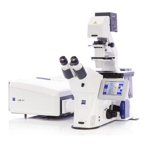
- Page 1 Training Guide for Carl Zeiss LSM 880 with AiryScan FAST ZEN 2.3 Optical Imaging & Vital Microscopy Core Baylor College of Medicine (2018)
- Page 2 Power ON Routine Turn ON ‘Main Switch’ from the Turn ON both ‘Systems/PC’ and Turn ON HXP-120V epi-fluorescence remote control paddle. ‘Components’ switches. light source. By default, the ‘Lasers’ key located This light source is required for on the side of the remote paddle visualizing fluorescence via the should always be in the ‘ON’...
- Page 3 Power ON Routine Turn ON HP Z840 PC. Double click ZEN Black icon to start When software has started, you will software. be presented with a login screen. Wait for PC to boot into Windows OS and login to ‘oivm’ user account. Note: Be sure to use Zen Black Select ‘Start System’...
- Page 4 Getting Started with ZEN 2.3 ZEN 2.3 is separated into three distinct areas. Image Acquisition Tools Represented by a group of blue bars each containing a series of tools for sample observation, image acquisition, image processing and system maintenance. Image Display This area is where each newly captured image will appear.
- Page 5 Getting Started with ZEN 2.3 5 – LSM 880 Training Guide...
- Page 6 Powering ON Lasers Before we begin setting up the software for imaging, we first need to verify that our lasers are powered on. There is a considerable wait time for the Argon laser to warm up (5 minutes) so please complete these steps first if the system is being powered on from an off state.
- Page 7 Mounting Sample on the Microscope While the lasers are warming up, we can mount our specimen on the stage above the microscope objective. 1. Place sample on microscope stage above objective (roughly in the center of the field of view). 2.
- Page 8 Mounting Sample on the Microscope 4. Via the microscope eyepieces, visualize your sample and adjust the focus (Z) and stage position (X,Y) accordingly. 5. Once a suitable location is found, click ‘ALL CLOSED’ from shortcuts (3). 6. Select ‘Acquisition’ from main toolbar to begin imaging. 8 –...
- Page 9 Light Path Configuration The confocal portion of the LSM 880 is equipped with a 34-channel spectral detector plus transmitted light and has 5 lasers with wavelengths 405nm, 458nm, 488nm, 514nm, 561nm, 594nm, and 633nm. The Light Path configuration allows you to program precisely how your image acquisition will be executed.
- Page 10 In the following example, we will design a sequential acquisition of two fluorophores (Alexa 568 and Alexa 488). Zeiss uses ‘Tracks’ to group a series of settings specific to a single fluorophore. Using sequential imaging, you should have one track for each fluorophore. These tracks can be switched in one of two ways: 1.
- Page 11 Light Path Configuration In the following example, we will design a 2 fluorophore (Alexa 568 and Alexa 488) sequential acquisition using the line-wise track switch. 1. From the Acquisition toolbar, expand the blue dialog labeled ‘Imaging Setup’ and set ‘Switch track every’ to ‘Line’. 2.
- Page 12 Light Path Configuration 7. Choose detector for imaging. Note: PMT selection will be based on where your fluorophore(s) fall in the linear range of the emission spectrum. Meaning that Ch1 typically corresponds to the lowest wavelength while Ch2 corresponds to the longest wavelength fluorophore. In our example, we will be using a sequential scan with Alexa 568 and Alexa 488, so Ch1(or ChS1) will be used for the Alexa 488 signal and Ch2 will collect the Alexa 568.
- Page 13 Acquisition Setup Once our light path setup has been completed we can expand the scanning tools to begin collecting an image. From ‘Acquisition Parameter’ there are 2 blue tabs used for imaging, ‘Acquisition Mode’ and ‘Channels’. Acquisition Mode This dialog controls static image settings such as: Objective –...
- Page 14 Acquisition Setup The ‘Channels’ menu contains the three components used to dynamically control image quality. They are (1) Laser Power, (2) Detector Sensitivity, and (3) Pinhole or Confocal Aperture Diameter. For further discussion on these parameters and how they affect image quality please see ‘Understanding Image Quality’ starting on page 19. Channels Functions available in the Channels dialog: Lasers –...
- Page 15 Scanning an Image Once the laser(s) have been turned on and our light path has been designed, we can scan an image and begin adjusting our signal level. 1. From the ‘Channels’ dialog, set the ‘Pinhole’ to 1 AU for the Track with the longest wavelength (Track 1 in this example).
- Page 16 Fine Tuning Image Quality In order to find the optimal settings for a particular condition, you must first be able to identify the thresholds of the signal level in the image. From the ‘Dimensions’ tab of the Image Display toolbar located below the image being scanned, you will find a checkbox labeled ‘Range Indicator’.
- Page 17 Fine Tuning Image Quality To fine tune the image intensity to ideal levels for final image acquisition: 1. Select one Track at a time – begin by highlighting the first Track in your list. Note: Make sure to uncheck all other tracks during this process so you are only scanning one color at a time.
- Page 18 Fine Tuning Image Quality Ideally, you do not want any area in the final image to contain blue pixels with this LUT. For maximum contrast, have the brightest areas fall just below overexposure (red) and the background areas fall just above underexposure limit (blue). In a properly balanced image you should see no blue pixels with this LUT.
- Page 19 Understanding Image Quality The result of the final scan above may or may not produce acceptable image quality. Therefore, it is important to have an understanding of the three key factors that play a role in image quality. Pinhole (Confocal Aperture) Laser Intensity Detector Sensitivity The confocal aperture controls...
- Page 20 Understanding Image Quality Pinhole (Confocal Aperture) Ideally, the confocal aperture should be set to the size of the structure(s) you are trying to resolve. However, for example, some sub-cellular structures of interest may be beyond Abbe’s diffraction limit and therefore beyond the microscope’s capability to resolve. The confocal aperture has some practical limits that can be used to guide the usage of this setting.
- Page 21 Understanding Image Quality Laser Intensity The overall power of the laser will directly affect image quality but most importantly it will have the greatest impact on the health of your sample and fluorophore(s). Increasing laser power will yield more signal but it will also induce negative photo effects such as phototoxicity and photobleaching that can harm the sample.
- Page 22 Understanding Image Quality Detector Sensitivity The sensitivity of the PMT is a function of the high voltage gain applied to it. The gain setting (as discussed elsewhere in this manual) controls the sensitivity of the detector to photons of light emitted from the sample fluorescence.
- Page 23 Understanding Image Quality Depending on the quality of the signal level in the final optimized image, you may find that the image is somewhat noisy. To compensate for this, the system has averaging functions in the ‘Acquisition Mode’ tab (page 14) that can be used to clean up the image.
- Page 24 Collecting a Z-Stack To collect serial sections (Z) we need to first activate the Z-Stack tools in ZEN which are hidden by default. 1. Check ‘Z-Stack’ from the experiment options. This will activate the Z Stack dialog in the Multidimensional Acquisition settings. 2.
- Page 25 Collecting a Time Series In order to collect a time-lapse (T) we need to first activate the Time Series tools in ZEN which are hidden by default. 1. Check ‘Time Series’ from the experiment options. This will activate the Time Series dialog in the Multidimensional Acquisition settings. 2.
- Page 26 Collecting a Tile Scan To collect tiled images for fields of view larger than a single frame, we need to first activate the Tile Scan tools in ZEN which are hidden by default. 1. Check ‘Tile Scan’ from the experiment options. This will activate the Tile Scan dialog in the Multidimensional Acquisition settings.
-
Page 27: Saving Images
Saving Images Once your image collection is complete you can save your data to the local hard drive. Along the right-hand side of the ZEN software (Region 3, page 6) you will find the list of images currently opened in ZEN. 1. -
Page 28: Shutting Down The System
Shutting Down the System 1. From the ‘Lasers’ dialog, select each laser that has been powered on and turn them off. Note: For the Argon laser, please wait 5 minutes before powering off the system electronics. 2. Close ZEN 2.3 application. Note: When prompted turn off the lasers –... - Page 29 Using AiryScan The AiryScan detection system is designed to increase the resolution and overall image quality compared to traditional confocal microscopy. The AiryScan is a single detector system – so compared to the confocal – it can only perform line switches for a maximum of 2 colors.
- Page 30 Using AiryScan 8. Select the appropriate emission filter for the fluorophore you wish to image. Note: The emission filters on the AiryScan are dual bandpass filters. These are configured with common combinations to limit the filter wheel from changing between tracks which can slow the system down. When choosing this filter, try to choose the best filter that matches two of your fluorophores.
- Page 31 Using AiryScan Once our light path has been designed, we can set up our baseline settings for the raw AiryScan data. In contrast to typical confocal imaging where you fill the dynamic range for optimal contrast; with AiryScan we want to set our sensitivity settings to fill 50% of the total available dynamic range.
- Page 32 Using AiryScan When we have finished balancing the available signal to fill 50% of the dynamic range, we can further prepare the system for scanning at the best possible resolution. 1. Go to Acquisition Mode and under Frame Size, click ‘Optimal’. Note: Using the Optimal feature is essential for sampling the field of view correctly for AiryScan.
- Page 33 Aligning AiryScan The initial alignment of the AiryScan must be checked each time you change your sample. Slight variances in sample prep, coverslip thickness and mounting media volume will influence the alignment so it is critical that this be checked for each new sample.
- Page 34 Aligning AiryScan 34 – LSM 880 Training Guide...
- Page 35 Aligning AiryScan 5. Allow scan to repeat until automatic alignment quality and status reads ‘Good’ OR until AiryScan detector view shows evenly illuminated array (as shown in example image). Note: Initially you may see the quality and status readout ‘Out of Range’ or ‘Bad’...
- Page 36 Processing AiryScan Data Once our RAW AiryScan data is collected – we must further process it to generate the final image. 1. Go to Processing tab and select ‘Airyscan Processing’ from method list. 2. Select previously scanned image as Input image. 3.
- Page 37 Using AiryScan FAST The AiryScan FAST detection system is designed for imaging with improved resolution at speeds that are significantly faster than traditional confocal – even with the base LSM 880. 1. From the Acquisition toolbar, expand the blue dialog labeled ‘Imaging Setup’. 2.
- Page 38 Using AiryScan FAST 8. Select the appropriate emission filter for the fluorophore you wish to image. Note: The emission filters on the AiryScan FAST are dual bandpass filters. These are configured with common combinations to limit the filter wheel from changing between tracks which can slow the system down. When choosing this filter, try to choose the best filter that matches two of your fluorophores.
- Page 39 Using AiryScan FAST Once our light path has been designed, we can set up our baseline settings for the raw AiryScan data. We start by deciding how we want to balance resolution with speed using the sampling frequency. 1. From the Acquisition toolbar, expand the blue dialog labeled ‘Acquisition Mode’.
- Page 40 Using AiryScan FAST In contrast to typical confocal imaging where you fill the dynamic range for optimal contrast; with AiryScan FAST we want to set our sensitivity settings to fill 50% of the total available dynamic range. 1. From the Acquisition toolbar, expand the blue ‘Channels’ dialog. 2.
- Page 41 Using AiryScan FAST 9. Snap Image. 10. Processing AiryScan FAST data – see page 36 for procedure. 41 – LSM 880 Training Guide...
Need help?
Do you have a question about the LSM 880 with AiryScan FAST and is the answer not in the manual?
Questions and answers