Cognex In-Sight 2000 Training Manual
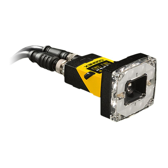
Vision sensor
Hide thumbs
Also See for In-Sight 2000:
- Installation manual (2 pages) ,
- Reference manual (57 pages) ,
- Manual (34 pages)
Table of Contents
Advertisement
Advertisement
Table of Contents

Related Manuals for Cognex In-Sight 2000


Summary of Contents for Cognex In-Sight 2000
- Page 1 Cognex In-Sight 2000 Training Provided by...
-
Page 3: Table Of Contents
Table of Contents Introduction: ..........1 Connecting to the IS2000 . -
Page 5: Introduction
Introduction: The In-Sight 2000 is a vision sensor, capable of providing a pass/fail output from the inspection of a part. It is easier to use than a full vision system but has capabilities beyond a basic photosensor or proximity sensor, or even an array of sensors. It uses the same software used for programming a Cognex In-Sight vision system, so you don’t need to learn a separate software to configure it. -
Page 6: Connecting To The Is2000
DHCP Server software on it (most computers don’t) then you need to assign the In-Sight 2000 and your computer static IP addresses. This section will show you how to do that. Launch In-Sight Explorer version 5.2.3 from the icon on your desk top if it is not already open. - Page 7 When this step is selected the pane just below it will appear as seen in Fig. 2. Any In-Sight system that is on the same subnet as the computer will appear here. If you have obtained an offline programming key, the name of your computer will appear in this pane followed by local emulator. This means that you can work with the software without being connected to an In-Sight vision system.
- Page 8 Fig. 3: Add Sensor/Device to Network The connected In-Sight 2000 should have been discovered and displayed in the list of devices. Click on the line that shows the unit to select it. From this dialog you can change the name of the unit if you desire.
- Page 9 Fig. 4: Add Sensor Message Box When the dialog closes you should now see your In-Sight 2000 listed in the pane showing In-Sight systems on your subnet (Fig. 2 on page 3). Click on it to select it and click the Connect button. You will see the software appearance change while attempting to connect to the In-Sight 2000 and after several seconds you will then see that it is connected.
-
Page 10: Set Up Image
Set Up Image Click on the Set Up Image application step button (Fig 5). When you do this the pane at the bottom will change to show the image acquisition settings. Fig 5: Application Steps - Set Up Image Fig 6: Image Acquisition Settings... - Page 11 The Delay control is disabled for this trigger type. The Manual trigger type allows the In-Sight 2000 to be triggered from In-Sight Explorer software. Both Delay and Interval are disabled for this type. Selecting Real Time Ethernet allows triggering...
- Page 12 Fig 9: Light and Exposure Settings The next section (Fig. 9) configures the intensity of the light and the exposure settings. First the exposure time can be set to a defined exposure time (Manual Exposure) or to a variable exposure time (Auto Exposure). The latter has two ways of calculating the exposure time and these are defined in the help files.
- Page 13 Fig. 10: Image Size The final section of this pane controls the size of the image that is captured (Fig. 10). The upper control in this section will set the number of rows that are captured in each image. This can be useful if the part does not move much in the field of view and cycle time must be reduced.
-
Page 14: Poker Chip Lab
Poker Chip Lab The first lab uses Cognex poker chips; each lab station should have a few of these chips. When developing an inspection you would follow the Application Steps from top to bottom to create a complete, fully functional inspection. - Page 15 In your system there are four tools that can be used for locating a part; in the other two models (lower cost and lower capability) of In-Sight 2000 only the Pattern tool is available. To the right of the list is a description of what the tool does and how to proceed adding it to your inspection.
- Page 16 Fig. 14: Locate Part - Pattern Tool The Model region appears pink, which signifies it is selected for editing. If the cursor is placed inside the rectangle it will appear as a white cross with arrowheads at each point. If you click and hold the left mouse button, the rectangle can be dragged to its desired location.
- Page 17 Fig. 15: Locate Part - Trained Model Placing the Model region close around the graphic on the chip allows defining edges to be trained while disregarding a significant amount of the background that could also contain significant variations. When choosing a pattern to use as a fixturing point you want something that would normally be present, is fairly unique and not too symmetrical, so that orientation of the found pattern is consistent and repeatable.
- Page 18 Fig. 16: Locate Part - Select Search Region Placing your cursor on the edge of the Search region and clicking the left mouse button will make it appear pink and the Model region will appear green (Fig. 16). At this point you could move and resize the Search region as you did with the Model region;...
- Page 19 Fig. 17: Locate Part - Accept Regions When the Model and Search regions have been set as desired, click the OK button in the Directions pane (Fig. 17) at the bottom of the window to accept the changes and finish adding the tool. When you click OK the tool will appear in the Results tab of the palette (Fig.
- Page 20 Fig. 20: Pattern Tool Settings - Name and Model Region On the right side of the Edit Tool pane are several entry fields and a control to retrain the Model should that be necessary. First you can assign a Name to the tool; while this is not required, as the software gives it a default name, it is a good practice to provide a descriptive name.
- Page 21 Fig. 21: Pattern Tool Settings - Angle and Acceptance On the left side of the Edit Tool pane (Fig. 21) are settings that relate to the manner in which the tool functions. In the upper left of this pane is an indicator that signifies if this tool passes or fails which is based on the tool settings and the runtime image.
-
Page 22: Inspect Part
For this lab leave the threshold at 50 and set the Rotation Tolerance to 180. Test your part location tool by placing the In-Sight 2000 into Repeating Trigger mode and moving and rotating the part within the field of view to assure that the part is found. If it is not properly located please ask for help. - Page 23 When this step is selected the Add Tool pane at the bottom of the window will appear showing the various tools available. The tools are grouped according to what they do and if you expand each group you would see the following (Fig. 23). The Presence/Absence Tools detect the presence of one object.
- Page 24 Fig. 25: Inspect Part - Pattern Regions The Model and Search regions can be moved and sized, as done with the pattern tool for locating the part, so that they appear similar to the image above (Fig. 25). Notice now that the search region is much smaller than was used for locating the part.
- Page 25 Fig. 26: Inspect Part - Pattern Settings At the right side of the Edit Tool pane (Fig. 26) we see the same controls that we saw in the same section of the pane for the part location tool but we also see an extra control, labeled Fixture. EasyBuilder automatically uses location information from the first part location tool added, to fixture other tools to the appropriate section of the part (this is why the search region can be kept small).
- Page 26 Before doing any testing you will add another tool; this time you will go back to the Add Tool pane and from the Absence/Presence Tools group you will select Pixel Count and click the Add button (Fig. 28). Fig. 28: Inspect Part - Pixel Count This time there will only be one region in the image.
- Page 27 Fig. 30: Pixel Count - Settings The right side of the settings pane for the pixel count tool has similar controls to the Pattern tool (without the image of the Model and the Model Region button). Consider naming this tool Chip Stacks.
-
Page 28: Inputs
For the purposes of the lab you have finished once you are satisfied with your results. In your process on the plant floor you would not be finished yet as you have not fully commissioned the system. The rest of this manual will serve as a reference for the rest of the application steps. Click on the next application step, Inputs (Fig. - Page 29 RAM so that it is the current inspection job. This requires that the job names stored in the In-Sight 2000 have a numerical prefix (0 to 31) so that a pulse train, of specific structure, can select the appropriate job. See the help files for the specific structure of the pulse train.
-
Page 30: Outputs
The next step is configuring the outputs. Click on the Outputs step (Fig. 33). Fig. 33: Application Steps - Outputs... - Page 31 When the Output application step is selected the output settings pane will appear at the bottom of the window. The In-Sight 2000 has four digital outputs and two LED’s on the body of the unit that can be configured. Each output can be given a name. Each output can be assigned a Signal Type of which there are multiple types too numerous to explain here;...
-
Page 32: Communications
Digital I/O is one way to control the In-Sight 2000 though it is not the only way. In-Sight systems can communicate over a number of industrial protocols including EtherNet/IP and ProfiNet. Control of the system and results from the system can be performed using industrial protocols so that no digital I/O is necessary. - Page 33 When the Communication step is selected the pane at the bottom will change (Fig. 37). This pane allows you to select and configure various communications paths. The EasyView selection allows configuration of the way data will appear on a VisionView panel if one is being used. If communications to a PLC/PAC or other industrial protocol gateway are to be configured click the Add Device button.
- Page 34 Fig. 39: Device Manufacturer Each of the controller manufacturers has protocols they support. Mitsubishi supports SLMP (a feature of CC-Link). Omron and Rockwell Automation both support EtherNet/IP and Siemens supports ProfiNet. Selecting Other offers the same choice of protocols listed above but the controller would come from some other manufacturer.
- Page 35 Fig. 41: Format I/O Data When the OK button is clicked a pane for setting the input and output data will appear with a tab for each of input data and output data (Fig. 41). Clicking the Add button at the lower left will open a dialog from which data can be selected (Fig.
- Page 36 In the Communication step you can also configure saving images from the system via FTP (File Transfer Protocol). From the first communications configuration pane (see Fig. 37 on page 30) select FTP. A new pane will appear in the bottom of the window with two tabs, Image and Settings. Click the Add button in the lower left corner of the Image tab to add an FTP Image connection (Fig.
- Page 37 Fig. 45: FTP Connection Settings On the Settings tab, two FTP connections can be defined (Fig. 45). These will set the path to the computer on which the FTP Server exists and provide access credentials for that computer. The FTP Settings button on the far right will open a dialog for defining the port and timeout settings along with allowing passive transfers over FTP.
-
Page 38: Filmstrip
Now that the job has been configured, I/O and communications have been set, just a few more steps that cover some essential information of how the inspection runs must be covered. The next application step is setting the Filmstrip. The Filmstrip is a feature that allows saving images from a system during troubleshooting or setup of the inspection. - Page 39 Fig. 47: Filmstrip Settings When the Filmstrip step is selected the pane at the bottom of the window changes (Fig. 47). The settings in this pane control which images are put into the queue (Pass/Fail/Pass and Fail), the size of the queue, the type of queue (Most Recent, First Only), the style of icon used to show which inspections pass and fail during runtime and a path where the images can be saved.
-
Page 40: Save Job
Now that you have tested your application, perhaps saved some test images, made any necessary changes to the job you are ready to deploy the system. Click on the Save Job application step (Fig. 50). Fig. 50: Application Steps - Save Job... - Page 41 Also in this pane you can set a Startup Job; if you have more than one job in your In-Sight 2000 this would specify the job that would be loaded when the system power is cycled. It is always a good idea to specify a Startup Job, even if you only have one job.
- Page 42 The final step is to run your job and inspect parts. Click the Run Job application step (Fig. 52). Fig. 52: Application Steps - Run Job...
- Page 43 Fig. 54: Run Job Results In the section with the controls you can place the In-Sight 2000 Online, clear the results counters, print the current results table, and set what is visible in the results table and image. You also see the current inspection rate and the time taken for the current inspection.
- Page 44 If the Options button is clicked a dialog opens that allows customization of the results table and the image (Fig. 55). Fig. 55: Results Display Options On the left side of the dialog are various check boxes that specify what is displayed in the results table.
-
Page 45: Logic Tool
In the inspection tools is a special tool that deserves its own explanation. Under the Math and Logic Tools group is one tool, Logic (Fig. 56). To insert the tool select it from the list and click the Add button. Fig. - Page 46 Expanding the list of the available tools exposes a pass and fail output from each (Fig. 58). Selecting an output will enable the Insert button; clicking the Insert button will insert the selected output into the expression field. Alternately you can double click an output to insert it. Fig.
- Page 47 Now that you understand how to use the software and have been guided through one lab it is time to try one on your own. If you have brought in parts to test you can use those to solve an application on your own.
Need help?
Do you have a question about the In-Sight 2000 and is the answer not in the manual?
Questions and answers