TA Instruments DHR Series Getting Started Manual
Small angle light-scattering (sals) accessory
Hide thumbs
Also See for DHR Series:
- Getting started manual (27 pages) ,
- Getting started manual (19 pages) ,
- Getting started manual (22 pages)

Related Manuals for TA Instruments DHR Series


Summary of Contents for TA Instruments DHR Series
- Page 1 DHR Series and AR Series Small Angle Light-Scattering (SALS) Accessory Getting Started Guide Revision G Issued November 2013...
- Page 2 TA Instruments may have patents, patent applications, trademarks, copyrights, or other intellectual prop- erty covering subject matter in this document. Except as expressly provided in written license agreement from TA Instruments, the furnishing of this document does not give you any license to these patents, trade- marks, copyrights, or other intellectual property.
-
Page 3: Introduction
Introduction Important: TA Instruments Manual Supplement Please click the TA Manual Supplement link to access the following important information supplemental to this Getting Started Guide: • TA Instruments Trademarks • TA Instruments Patents • Other Trademarks • TA Instruments End-User License Agreement •... -
Page 4: Notes, Cautions, And Warnings
Notes, Cautions, and Warnings This manual uses NOTES, CAUTIONS, and WARNINGS to emphasize important and critical instructions. In the body of the manual these may be found in the shaded box on the outside of the page. NOTE: A NOTE highlights important information about equipment or procedures. CAUTION: A CAUTION emphasizes a procedure that may damage equipment or cause loss of data if not followed correctly. -
Page 5: Electromagnetic Compatibility Standards
Electromagnetic Compatibility Standards For Australia and New Zealand AS/NZS CISPR11:2004 Limits and methods of measurement of electronic disturbance characteristics of industrial, scientific and medical (ISM) radio frequency equipment. For Canada ICES-001 Issue 4 June 2006 Interference-Causing Equipment Standard: Industrial, Scientific, and Medical Radio Frequency Generators. -
Page 6: Safety
120/240 volts AC are present in this system. WARNING: High voltages are present in this instrument. Maintenance and repair of internal parts must be performed only by TA Instruments or other qualified service personnel. AVERTISSEMENT: Présence de tensions élevées dans cet instrument. La maintenance et la réparation des pièces internes doivent être effectuées... - Page 7 Please heed the warning labels and take the necessary precautions when dealing with those parts of the instrument. This manual is intended to be used in conjunction with the DHR Getting Started Guide and the AR-G2/AR 2000ex/AR 1500ex Rheometer Getting Started Guide. For full details on the operation of the rheometer and safety information, please refer to that manual.
-
Page 8: Table Of Contents
Important: TA Instruments Manual Supplement ........ - Page 9 Chapter 4: Using the SALS Accessory .................... 32 Overview ..............32 Loading the Sample .
-
Page 10: Chapter 1: Introducing The Sals Accessory
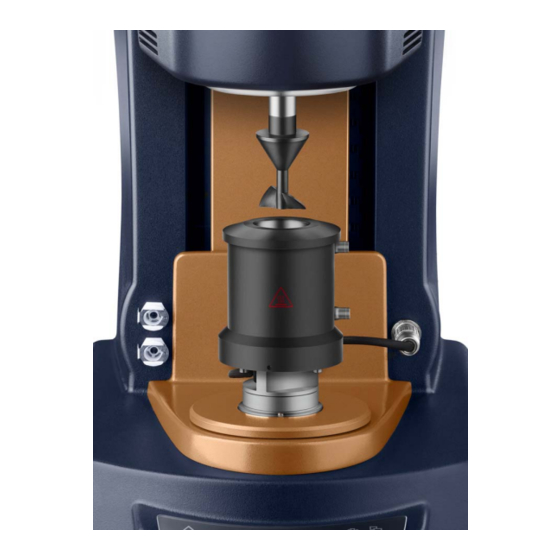
Figure 1 SALS Accessory. The TA Instruments SALS Accessory is a Smart Swap™ system designed for use with the DHR-3, DHR- 3, and AR-G2/AR2000ex Rheometers. A patented, Peltier temperature-controlled lower plate, with sap- phire window, allows the laser to be trained on the sample. The resultant scattered light is transmitted through the upper transparent quartz geometry and is observed by a lens and camera assembly. -
Page 11: The Direction Of Incident Light
In principle, the incident light can be in any direction relative to the shear direction, but it is usual to arrange it along one of the principle axes. In the TA Instruments system the shear gradient direction is used, so scattering occurs in the plane of the vorticity (neutral) direction - shear direction (see below). -
Page 12: Product Description
Product Description The laser used in the SALS Accessory is a Class II 0.95 mW diode laser, wavelength 635 nm, circular beam with diameter of 1.1 mm, beam divergence (typical) 0.7 mrad. The upper geometry is a 50 mm diameter x 2 mm thick optical quartz disk, refractive index 1.457 at 635 nm. -
Page 13: Adjusting The Plane Of Focus
Figure 5 Schematic of TA Instruments SALS optics. The position of the PCX lens is indicated by the inscribed scale. One rotation of the lens holder is equiva- lent to a travel distance of 1 mm. The zero position is assumed to be where the DCX and PCX lens are in contact. -
Page 14: Polarization
Polarization The diode laser used produces plane polarized light. In the TA Instruments system, the direction of polar- ization is aligned with the shear direction. An analyzer (i.e., a second polarizer) is placed in the path of the diffracted light. There are two positions for the analyzer, parallel or perpendicular to the direction of polar- ization of the incident beam. -
Page 15: Specifications
Specifications Table 1: SALS Accessory Specifications q Vector Range ~1.38µm to 6.11µm Scattering Angle ~6° to 26.8° Laser 635nm 0.95mW class 2 Peltier Temperature Controlled 5 to 95°C WARNING: The upper temperature limit is set by the optical adhesive that retains the sapphire window. -
Page 16: Chapter 2: Installing The Sals Accessory
Chapter 2: Installing the SALS Accessory Installing the SALS Accessory The steps needed to attach the SALS Accessory to the rheometer involve the following: Mounting the upper and lower fixtures Attaching the upper geometry Connecting camera and installing drivers Aligning the system Mounting the Upper and Lower Fixtures Follow these steps to mount the fixtures: Ensure that the rheometer is turned on. -
Page 17: Connecting The Camera And Installing The Drivers
Connecting the Camera and Installing the Drivers To get your camera up and running, follow these steps before plugging in the camera USB cable: Download the LuCam Software V6.0.3 or higher from the link below: http://www.lumenera.com/support/downloads/industrial-downloads.php Run the downloadable executable LuCamSoftware-v6.0.3.exe and follow the instructions given. Once installed, plug in the camera to a spare USB port and follow the instructions to install from the “recommended”... -
Page 18: Aligning The System
Aligning the System The laser in the base and the surface of the Peltier Plate are factory aligned and should not require any adjustment. A small amount of adjustment will be necessary to align the upper fixture whenever it is fitted. This is most easily achieved by using a sample with a known scatter pattern. - Page 19 Ensure the polarizer ring (analyzer) on the upper fixture is set to “in parallel.” This is when the ring is rotated fully up, as shown in the image below. Figure 9 Polarizer ring. Remove any neutral density filter from the drawer in the lower fixture. See Figure 10 below.
- Page 20 13 Adjust the body of the upper fixture in the swivel mount (see below, left) until you obtain a pattern of concentric rings similar to those shown in the below-right image. Figure 11 Swivel mount. NOTE: It may be necessary to adjust the camera settings such as exposure, brightness, and contrast by accessing the Camera properties on the camera setup screen (right-click on image).
-
Page 21: Chapter 3: Calibrating The Sals Accessory
Chapter 3: Calibrating the SALS Accessory Preparing the SALS Before starting an experiment you need to decide what you want to learn from the scattering data as this will impact greatly on the amount of calibration and data treatment required. The simplest use (level 1) might be to collect the scattering image during an experiment, and then look at anisotropy in the image to infer structure changes within the sample that match features in the rheological data. -
Page 22: Calibrating The Scattering Angle
Calibrating the Scattering Angle Calculation of the Scattering Angle The relationship between the scattering angle and the pixel position on the sensor can, in principle, be cal- culated directly from the characteristics of the optical system, but variables such as the lens and sensor positions are not known sufficiently precisely to make this a reliable way of determining that relationship. -
Page 23: Using The Laven Program
The Laven program main window is shown below. Some of the information that needs to be entered is given on the Certificate of Analysis supplied with the microparticles. The other entries are either standard values or are specific to the TA Instruments SALS system. Figure 13 Laven program main window. - Page 24 Polarization. Select as appropriate. Either perpendicular or parallel options can be used with TA Instruments SALS system. For the remaining two text boxes, select Mie and Intensity v. scattering angle.
-
Page 25: Preparing And Loading The Calibration Sample
Preparing and Loading the Calibration Sample Follow steps 1 to 12 of the alignment procedure, lock the camera exposure, and then capture the image. To improve the data quality, it is best to record several images at this point, for later averaging. An oscillatory time sweep at the minimum stress in continuous controlled stress mode is suitable for this task. - Page 26 Enter the desired values and click OK. The averaged image should resemble that shown below. A similar process can be used to obtain a background image for water. Figure 16 Averaged Mie scattering image in ImageJ. Once you have both averaged images, the background is subtracted using the Image Calculator window (shown below) selected from the Process menu.
- Page 27 Choose Plugins>Radial profile angle. The window shown below displays. Figure 18 Radial Profile Angle window from ImageJ. Input the radius over which the integration is to be performed, in pixels. To take full advantage of the camera chip, this should be set to 512. The integration angle is on both sides of the starting angle, so the full angle is twice that entered.
- Page 28 10 Click Calculate Radial Profile, and an image similar to the one below displays. The plot is intensity against distance from the center point, in pixels. The intensity is adjusted to account for the increase in the number of pixels with increasing radius, but further corrections need to be made for the sensor properties and solid angle.
-
Page 29: Calculating The Optics Correction Factor
Calculating the Optics Correction Factor The two system calibration factors are determined using a worked example in Excel. This section shows a worked example using Microsoft Excel, Laven data and Intensity vs. Radius (pixels) date from ImageJ. Open the .txt file created by the Laven program in Excel. See the figure below. Figure 20 Excel spreadsheet displaying Laven data. - Page 30 Add the data below into the cells indicated, copying the formulae down to line 385. Radius Intensity Angle Correction corr shift [pixels] Factor =(180/ =(L2*J$2)/P2 =(COS(M2*PI()/ PI())*ATAN(K2*G$5) 180)) =(180/ =(L2*J$2)/P2 =(COS(m2*PI()/ PI())*ATAN(K2*G$5) 180)) Also add the optics factor at G5. This value, together with the y shift, is approximate and will be modified later.
- Page 31 Paste the data from ImageJ into columns K and L. Figure 22 Data pasted. Create a xy overlay graph of D vs. A and N vs. M. Scale the y axis to 5000 maximum. Adjust the y shift so that the first peaks of each curve have the same maximum. Adjust the Optics Factor so that the first peaks of each curve overlap.
-
Page 32: Chapter 4: Using The Sals Accessory
Chapter 4: Using the SALS Accessory Overview Once the SALS accessory has been properly installed, aligned, and calibrated (if needed), follow the direc- tions in this chapter to load your samples, set the focal positions, lock the exposure, and select the desired image format for your results. -
Page 33: Setting The Focal Position
Setting the Focal Position It is not essential to use a geometry gap of 1000 microns, but it is important that the focal position be within the sample. The table below shows the approximate depth of the focal point within the sample, pre- dicted for a sample of refractive index 1.333 (i.e., equal to that of water), for the adjustable front lens posi- tions taken from the scale. -
Page 34: Index
Index cautions 4 ImageJ using 25 instrument symbols 6 license agreement 3 loading the sample 32 locking exposure 33 notes 4 patents 3 Regulatory Compliance 4 safety 6 instrument symbols 6 Safety Standards 4 SALS aligning system 18 calibrating 22 installing 16 loading the sample 32 overview 10... - Page 35 25 product description 12 setting the focal position 33 specs 15 using 32 scattering theory 10 setting the focal position 33 TA Instruments offices 3 trademarks 3 warnings 4 DHR/AR Series SALS Accessory Getting Started Guide Page 35...
Need help?
Do you have a question about the DHR Series and is the answer not in the manual?
Questions and answers