Table of Contents
Advertisement
Quick Links
Advertisement
Table of Contents

Related Manuals for Harvard Bioscience Multi Channel Systems Smart Ephys CMOS-MEA5000


Summary of Contents for Harvard Bioscience Multi Channel Systems Smart Ephys CMOS-MEA5000
- Page 1 CMOS-MEA5000-System Manual...
- Page 2 Imprint Information in this document is subject to change without notice. No part of this document may be reproduced or transmitted without the express written permission of Multi Channel Systems MCS GmbH. While every precaution has been taken in the preparation of this document, the publisher and the author assume no responsibility for errors or omissions, or for damages resulting from the use of information contained in this document or from the use of programs and source code that may accompany it.
-
Page 3: Table Of Contents
Table of Content 1 Important Safety Advice ......................5 1.1 Guarantee and Liability ......................6 1.2 Operator's Obligations ......................6 2 Introduction ........................... 7 2.1 Welcome to the CMOS-MEA5000-System ................. 7 3 Hardware ............................8 3.1 Headstage ..........................8 3.2 Chip Orientation inside the Headstage………...…...……………………………………………….8 3.3 CMOS-MEA Chip ........................ - Page 4 10.2 Results View ........................113 10.2.1 Toolbar ........................113 10.2.2 Units List ........................115 10.2.3 Filters and Sorting ..................... 116 10.2.4 Chip Overview ......................117 10.2.5 Unit Comparison ...................... 118 10.2.6 Unit Details ....................... 119 10.3 Spike Sorter Settings ......................122 10.3.1 ROIs ..........................
-
Page 5: Important Safety Advice
1 Important Safety Advice Warning: Make sure to read the following advice prior to installation or use of the device and the software. If you do not fulfil all requirements stated below, this may lead to malfunctions or breakage of connected hardware, or even fatal injuries. Warning: Always obey the rules of local regulations and laws. -
Page 6: Guarantee And Liability
Requirements for the Installation Make sure that the device is not exposed to direct sunlight. Do not place anything on top of the device, and do not place it on top of another heat producing device, so that the air can circulate freely. Explanation of the Symbol used Caution / Warning DC, direct current... -
Page 7: Introduction
2 Introduction 2.1 Welcome to the CMOS-MEA5000-System Multi Channel Systems is proud to present the CMOS-MEA5000-System. Based on the complementary metal-oxide semiconductor technology, it opens up new possibilities in electrophysiological research. With more than 4000 recording sites, each of them sampled at up to 25 kHz, the chip allows extracellular recordings at a very high spatio-temporal resolution. -
Page 8: Hardware
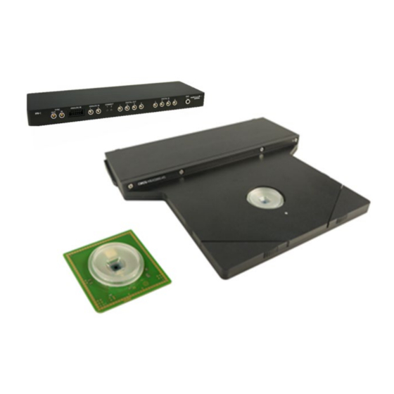
3 Hardware 3.1 Headstage There are three hardware components for the CMOS-MEA5000-System available, the headstage, the interface board and the data acquisition computer. If necessary you can use a temperature controller additionally. For setting up and connecting the CMOS-MEA5000-System, please read the next chapter "Hardware Setup"... -
Page 9: Cmos-Mea Chip
3.2 Chip Orientation inside the Headstage If you are stimulating with light or extra electrodes from outside the chip, or if the orientation of the tissue is important, please be aware that the line of vision is from the headstage side where the connector to the IFB is located. - Page 10 The CMOS-MEA chip has a 65 x 65 layout and is available with 16 μm or 32 μm interelectrode distance (center to center). The electrode diameter is always 8 μm. Between the recording electrodes, there is a grid of 32 x 32 bigger stimulation sites. Summarizing, you can record from 4225 electrodes and stimulate your sample at 1024 sites.
- Page 11 At the moment three types of culture chambers are available for CMOS-MEAs: One for cell cultures and two for acute slices. The chips for acute slices need an external Ag/AgCl electrode to ground the bath. This ground electrode is already integrated in the CMOS chip for cell cultures. CC Culture chamber for cell cultures with lid.
-
Page 12: Ifb-C Multiboot Interface Board
3.4 Interface Board IFB-C The multiboot interface board IFB-C facilitates operation of all MCS in vitro and in vivo headstages within the entire 2100 amplifier solution suite. This suite includes: MEA2100-HS, Multiwell-MEA-HS, CMOS- MEA-HS, MEA2100-Beta- Screen-HS, W2100-HS and ME2100-HS. The modular 2100 amplifier solution suite design makes it easy to modify your lab equipment generally with modest hardware upgrade investments. - Page 13 If access to more bits of the DIG IN / OUT channel is required, it is necessary to connect a Digital IN / OUT extension Di/o board with a 68-pin standard cable. This Di/o board is available as optional accessory. Ground If an additional ground connection is needed, you can connect this plug with an external ground using a standard common jack (4 mm).
- Page 14 Digital IN / OUT A Digital IN / OUT for 16 digital in- and output bits is available via Honda-PCS-XE68LFD connector. Please read chapter Digital IN / OUT Connector in the Appendix for more information about the pin layout of the connector. The Digital IN / OUT connection accepts or generates standard TTL signals. The Digital OUT delivers TTL pulses with 3.3 V or 5 V.
- Page 15 Data Acquisition Computer The software CMOS-MEA-Control was programmed specially for the CMOS-MEA5000-System. It facilitates a real-time activity overview on the complete chip with the ability to zoom in and various tools to analyze the data. Please read chapter "CMOS-MEA-Control" for information about the software. The data acquisition computer is provided by Multi Channel Systems MCS GmbH.
-
Page 16: Hardware Setup
4 Hardware Setup Please follow the instructions: Connect the CMOS-MEA5000 amplifier via iX-industrial cable, type B to the IFB-C interface board. Please use the plug in labelled with “1” on the back of the interface board. Connect the IFB-C via power unit to the power outlet. Connect the IFB-C via USB-C to the computer. -
Page 17: Installation Of The Software
5 Installation of the Software 5.1 System Requirements If you have purchased the CMOS-MEA5000-System with PC everything is preinstalled and tested. If you purchase a system without a PC please make sure that the computer meets our specifications relating processor, memory, hard disk, etc. Please contact Multi Channel Systems MCS GmbH or your local retailer. -
Page 18: Testing The Cmos-Mea5000-System
5.2 Testing the CMOS-MEA5000-System Functional Tests of the CMOS-MEA5000-System with the Test Model Probe Please read also the datasheet “Test-CMOS-MEA” in the Appendix. Insert the "Test Model Probe" in correct orientation and close the headstage. The round edge of the Test-CMOS-MEA or the CMOS-MEA chip has to be in the front on the left side when looking directly to the open amplifier. - Page 19 Test of the internal Stimulators The Test-CMOS-MEA probe is equipped with three additional connectors to test the internal stimulation, „STG1“, „STG2“ and „STG3“. The stimuli are color coded in the CMOS-MEA-Control software: Stimulus 1 is indicated in green color, Stimulus 2 is indicated in blue and Stimulus 3 in red color. For testing a stimulator, please connect the cable of the "ODD"...
- Page 20 CMOS-MEA Chip Please fill the CMOS-MEA chip with PBS and add an external reference electrode. CMOS sensors are light sensitive. To record a stable baseline the CMOS-MEA array must maintain under stable light conditions, which can easily be provided by covering the CMOS-MEA with the convenient dark chamber “CMOS- DC”.
-
Page 21: General Software Features
6 General Software Features The chapter "General Software Features" describes some of the CMOS-MEA-Control and CMOS-MEA- Tools software features on base of examples. Numeric Up-Down Box Adjust a value in the numeric up-down box either by clicking on the arrow buttons or by clicking into the window and moving the mouse wheel. - Page 22 Display Floating Design your own display with the floating feature. Decouple a dialog display of your choice and place it wherever you want. Dock the window again by clicking with the right mouse button on top of the window. Hide a window with the "Auto-Hide" option. Creating Regions of Interest ROIs Selecting ROIs manually by drawing rectangles is identical even in the "Activity"...
-
Page 23: Cmos-Mea-Control Software
7 CMOS-MEA-Control 7.1 Introduction The software for controlling the CMOS-MEA5000-System includes two parts, CMOS-MEA-Control for online recording, CMOS-MEA-Tools for offline analysis. The CMOS-MEA-Control software is explicit designed for online data recording with the CMOS- MEA5000-System. It facilitates a real-time activity overview on the complete chip with the ability to zoom into the raw data and various tools to visualize the activity. -
Page 24: Menu Bar
The default window of the main menu is divided in three parallel sections which are framed by the menu bar above: 1. Left: Control section to control the CMOS-MEA5000-System hardware, the data acquisition, the experimental procedure, the recording of data, the streaming of detected spikes and a section to monitor the system load. - Page 25 Click "Set Default Folder" to open the "Application Settings" dialog. Define the paths for the "Default Paths" for "Raw Data", "Template" and "Stimulation Files" in the "Application Settings" dialog. Important: Make sure that all paths go to the SSD drive otherwise no recording is possible! Click the check box “Save Sensor Calibration”...
- Page 26 Setup Click "Device" to change the connected device. If hardware is available, choose the "MCS Device". If no hardware is available, please use the "Simulator" or load a "Data File" to test the software without hardware attached. When replaying a data file, you have the advantage to see "real" data meanwhile the data of the "Simulator"...
- Page 27 Open the "Device Filter" dialog to change filter settings. Adjust the settings of the "High Pass" and "Low Pass" filter on hardware level during the software is running, but not recording. Choose "Bessel" or "Butterworth" filter "Family" in 1 or 2 "Order" from the drop-down menus.
- Page 28 If the software is not up to date, click the button "Visit Web site" and download the newest software version. The "Help" menu is for opening the online help "CMOS-MEA-Control Help" and to "Download Update", if necessary. Click the "About" option for software and firmware information. Please see technical specifications of the device and the version number of the CMOS-MEA-Control software.
-
Page 29: Control Section
7.4 Control Section The "Control Section" includes three sections, the "Data Source", the "Recorder" and the "Load" control. Data Source The "Data Source" window allows controlling the data source and the CMOS chip. The chip is an active device and has to be powered before you are able to start an experiment with the "Start" button. Click the "Settings"... - Page 30 Recorder Control the "Recorder" parameter settings in this window. Start and stop the recorder and see the types of data available. Press the "Settings" icon to change recorder settings. Please read chapter "Operating CMOS-MEA-Control" for detailed information about programming the recorder. Start and stop the recording manually with the "ON / OFF"...
- Page 31 Spike Server The "Spike Server" allows to stream detected spikes and events to other applications on the same computer or to another computer in the network. The client receives the data and can process it to the needs of the customer. We provide source code for such a client in C#, Matlab and Pythen. Load Monitor the current state of the capacity of the data acquisition computer via "Load"...
- Page 32 Sensor Current See the "Sensor Current" of the CMOS chip. The sensor current is measured as the sum of all current over all 4225 sensors. The total current should not be larger than about 300 mA, otherwise the chip get damaged.
-
Page 33: Data Display
7.5 Data Display 7.5.1 Activity Due to the high number of channels, it’s impossible to show raw data of 4225 channels simultaneously. Therefore, activity is visualized in time bins in a false color code. This allows the user to identify active areas and to focus on them in regions of interest. - Page 34 Creating Regions of Interest ROIs Please keep the left mouse button pressed to draw a rectangle in the "Activity" window to create a region of interest. A dashed line in blue indicates the borders of the ROI. The color of the rectangle turns to black and the number of the ROI appears in the upper right edge.
- Page 35 Upper Toolbar of the "Activity" Window Click the "Parameter Selection Icon" icon to decide which parameter mode of the sensor activity should be displayed: The maximal "MaxAmplitude" or the "MeanAmplitude or the "SpikeCount". In dependency of your choice, the toolbar beside changes. The selected parameter will be shown in the activity window as false color plot in time bins.
- Page 36 Lower Toolbar of the "Activity" Window If the mouse pointer is positioned on the map, the coordinates of the area the mouse is pointing at is shown at the left side of the toolbar below the plot window. Define the color of the "Activity Map" by clicking the second setting icon in the toolbar below.
-
Page 37: Sensor Array Tool
The color depicts the selected parameter in the "Activity" display. As seen in the image below, activity is shown as colored spots. 7.5.2 Sensor Array Tool The "Sensor Array Tool" integrates three functions which are related to the control of the CMOS-MEA chip. - Page 38 Calibration As mentioned above the condition of the sensor chip can be estimated by the conversion factors obtained during the system calibration. Each sensor's calibration value is represented by a color coded dot. The exact values depend on the sensor chip. The pattern of this values should be a kind of random noise pattern.
- Page 39 Sensor Selection The "Sensor Selection" module allows the user to select regions of interests manually or automatically. It is useful to reduce the amount of data transferred to the computer and to hard disk when the activity is restricted to one or several locations of the sensor array. Fetch the activity distribution obtained by the "Activity"...
- Page 40 Upper Toolbar of the "Sensor Array Tool" Window Please download your selection of regions of interest with the "Download the Selected Sensors to Data Acquisition" button to the computer. Use the "Fetch Spike Count from Spike Tool" button to import data from the "Spike Tool"...
- Page 41 The "Sensor Reset" tool raises the floating signals back to the operation point. This short period is visible in the raw data as a potential step. The exact time of the reset is recorded together with the raw data as channel data or as events.
- Page 42 Example: "Sensor Reset" with suppression The example above on the left shows a sensor reset with an interval of 1 ms, with 10 Hz filter and with suppression. The example above on the right shows a sensor reset with an interval of 1 ms, without filter and with suppression.
-
Page 43: Spike Tool
7.5.3 Spike Tool The "Spike Tool" is used for the online determination of spike parameters to allow an activity dependent recording. This is useful when active phases are embedded in long inactive phases. Using this feature just the interval around active phases are stored on disk. Spike Tool upper Toolbar Define the "Threshold"... - Page 44 Click the "Open Settings Dialog" button to open the "Spike Explorer Settings" dialog. Spike Detection Please define various parameter for the spike detection. The noise is used as a base to calculate the threshold of the spikes which should be detected. Noise Measure Section "Noise Measure"...
- Page 45 Detection Section "Detection" parameter: Define the "Threshold Type" from the drop-down box, "Positive", "Negative" or "Absolute". It is also possible to define this parameter in the tool bar of the "Spike Tool" display. Select the "Threshold" from 0 to 99 from the up-down box. Define the "Detection Dead Time" in ms. Spike Cutout Section "Spike Cutout"...
-
Page 46: Stimulation
Spike Tool Event Window See the spike rate in dependency of the time in the "Spike Tool Event" window and adjust the threshold to trigger events by moving the red bar with the mouse. When the spike rate crosses the threshold in positive direction, a specific positive “Spike Rate Threshold” event is created and dispatched. -
Page 47: Analog Channels
7.5.5 Analog Channels Eight analog "Analog Channels" are available to record additional analog signals. Start and stop the analog displays separately. Use the toolbar to customize the zoom factor and the timeframe for the data. Please read also chapter "General Display Features". 7.5.6 Digital Port Events Digital events can be generated on TTL pulses coming in on the "Dig In"... -
Page 48: Detailed View: Region Of Interest
7.5.7 Detailed View: Region of Interest Define one or more regions of interest in the "Activity" display on the left side of the main menu. If more than one ROI is available, please see the tabbed pages in the detailed view. Do not choose too much sensors for the detailed view, because displaying the single sensors needs very much computer performance. -
Page 49: Single Sensor View
7.5.8 Single Sensor View Select one of the electrodes of the ROI for a closer look. Start and stop the "Single Sensor View" separately to save computer performance or to have a closer look. Use the toolbar to customize the zoom factor and the timeframe for the data. Please read also chapter "General Display Features". -
Page 50: Operating Cmos-Mea-Control
8 Operating CMOS-MEA-Control Software If a device is not recognized automatically after starting the CMOS-MEA-Control Software, please click the "Settings" icon in the "Data Source" window for the "Set Device" dialog and select the connected CMOS device. This can happen at the first use on a specific data acquisition computer, or after upgrades. - Page 51 Clicking the chip icon opens additional to powering the chip the "Automatic System Calibration" dialog. The following important steps for calibration are performed automatically. Please see the protocol log file to monitor the process. 1. Set sensor operation point. 2. Wait until the signals stop drifting. 3.
- Page 52 Chip Power Window After powering the CMOS-MEA chip, you will find information about the voltage applied to the chip, displayed in the up-down boxes. The user is not allowed to change these voltage levels. Set Sensor Operating Point Window Please set the sensor operating point in mV. Standard values for the "Source-Drain" and the "Source- Gate"...
- Page 53 The offset for each single sensor should be approximate to zero. The voltage needed for this ADC offset is displayed in the "Input Offset" up-down box in mV. You can observe the process in the ROI display and in the single view. Minimize Floating Artefact Window Define the voltage in "Source-Bulk"...
- Page 54 Sensor Calibration Window The input voltage of each transistor correlated to the sensors are different. The "Sensor Calibration" function sets the input voltages to a common level. The stimulation of the bath is the first step, then measuring and evaluation. Bath Stimulation Window Independent from the stimulation of electrodes it is possible to stimulate the bath itself.
-
Page 55: Recording
8.1 Recording The CMOS chip includes 4225 recording electrodes and 1024 stimulation sites. The 16 μm interelectrode distance chip offers the highest resolution. With the high number of electrodes, you can record from a large surface (1 mm² @ 16 μm distance, 4 mm² @ 32 μm distance). Thereby, you can see the signals from every single cell and even the signal propagation along an axon, while still getting an overview on your complete sample. - Page 56 hand. The combination of different modes offers a lot of possibilities to record data focused on critical periods. Starting and Stopping the Recording "Manual". Please click the "On" / "Off" button on top of the "Recorder" dialog manually. Starting and Stopping the Recording via "Timer".
- Page 57 Starting and Stopping the Recording via "Event". Using an "Event" as start and stop trigger postulates to build this event before. An "Event" may be a digital TTL trigger coming from external or an internal TTL marker signal programed with a stimulation pattern.
- Page 58 The stimulation pattern appears like this, for example. The marker signal is the orange trace, shown in the lower display of the complete stimulus pattern. Please define a "Marker Port" for delivering the TTL signal.
- Page 59 Spike Rate triggered Recording The functionality of the “Spike Tool” and the “Recorder” allow an activity dependent recording. This is useful when active phases are embedded in long inactive phases, for example for epilepsy research. Using this feature just the interval around active phases are stored on disk. The “Recorder”...
- Page 60 To make the analysis more specific just select the sensors which show the behavior you are interested in. Restricting the analysis to a few sensors of a distinct temporal spike pattern you can reduce the noise originating from all other sensors with uncorrelated activity. The threshold (red line) can be moved by mouse.
-
Page 61: Stimulation
8.2 Stimulation Warning: Only positive voltages should be applied to the CMOS arrays. Negative voltages will damage the chip. Changing voltages will generate a current. Default pulse form is therefore a positive voltage ramp. Warning: Do not use voltages higher than 3.4 V, or you will damage the CMOS array. Stronger voltages will lead to a breakdown of the isolation layer. - Page 62 Tool Bar The tool bar in the "Stimulation" window is divided into three sections: A position indicator, controls for single stimulus patterns, and controls that affect all three stimulus patterns. The function of all icons is explained via tool tip, when you move the mouse over the icon. First section: The position indicator helps to navigate through the CMOS-MEA electrodes.
- Page 63 For displaying the "Activity Map" window, please use the "Display Activity Map" button. Third section: To clear all sites, click the "Clear all stimulus sites" icon. Start all stimulus patterns simultaneously via the "Start" icon in this section. To open the "Define Stimulus 2" dialog, click the "Select Stimulus 2" icon .
- Page 64 The "Define Stimulus" dialog is divided in an upper and a lower section. The upper part includes the "Primitives", that means, the icons for the provided stimulus patterns, such as flat line, ramp or sine waves. The last icon represents ASCII files generated by a different software, for example MC_Stimulus II, which can be imported into the CMOS-MEA-Control software.
- Page 65 Setting a Marker Signal Additionally it is possible to set a marker signal. Open the "Set Marker Signal" dialog by clicking the check box "Set Marker" in the window for parameter settings. Click the check box "Set Marker" and click "Repeat" if you want to repeat the marker signal at each cycle of the stimulation pattern.
- Page 66 Stimulus Pattern: Flat Line The first provided primitive is a flat line stimulus. To adjust the duration, please use the respective up-down boxes: Hour, minute, second, millisecond and microsecond. Define the value of the pattern in the "Amplitude (mV)" up-down box.
- Page 67 Stimulus Pattern: Sine Wave Warning: Negative voltages will damage the CMOS arrays. Sine waves must be shifted with an offset to positive range! Modulate the amplitude "PP Amp (mV)", the period "Period (μs), the shift "Shift" and the phase "Phase (') of the sine wave pattern via up-down boxes.
- Page 68 Stimulus Pattern: Ramp The equivalent of a biphasic current pulse is a triangular voltage ramp. About 9 stimulation pads (3x3) minimum are needed for an effective stimulation (valid for retina, no data yet for cell culture). In contrast to regular MEAs, neighboring recording sensors will usually NOT saturate during stimulation, so recording in very close proximity to the stimulation site is possible.
- Page 69 Stimulus Pattern: Biological Pulse via ASCII Import Warning: Negative voltages will damage the CMOS arrays. Sine waves must be shifted with an offset to positive range! Important: The resolution of the stimulator is 10 μs in time axis and 105 μV in voltage. The stimulus generator is not able to release pulses shorter than 10 μs or lower than 105 μV, therefore such pulses are skipped! If you like to use, for example, a biological signal as stimulus pulse or you want to create an arbitrary...
- Page 70 If the import file does not meet the requirements, an error message is shown.
- Page 71 Stimulus Pattern: Biological Pulse Example: Import of the following file as stimulation pattern: Note: Because the slope of the signal determines the strength of the induced current, please add ramps to the start and stop of the biological signal to avoid stimulation artefacts.
- Page 72 Stimulation Pattern: Loop Place any stimulus pattern between a "Loop" primitive and the patterns can be repeated as often as needed. Please select the number of looping "Cycles" from the up-down box. The "Loop" primitive is not movable in the sequence of the stimulus patterns. Drop it into the bin and start again to change the position of the "Loop"...
- Page 73 Tool Bar The settings in this tool bar influence the complete sequence of the stimulus patterns. Modulate the “Amplitude (%)” and the “Offset (mV)” of the complete pattern via up-down boxes. Clicking the "Loop" button enables you to infinitely repeat the defined stimulus pattern. Load a previous created stimulus pattern, save or delete the pattern.
-
Page 74: Cmos-Mea-Tools
9 CMOS-MEA-Tools Introduction The software for controlling the CMOS-MEA5000-System includes two parts, CMOS-MEA-Control for online recording and CMOS-MEA-Tools for offline analysis. With Multi Channel DataManager software you can export data to third party applications. 9.1 Main Window The default window of the start menu is divided in two main sections: The "Control Window" and the "Data Display or Settings Window". -
Page 75: Menu Bar
9.1.1 Menu Bar File Menu to import raw data for analysis: "Open Raw Data File" with the extension "*.cmcr" created with "CMOS-MEA-Control" software for analysis and to "Exit" the program. Menu to "Load Result File" with the extension "*.cmtr" for reanalysis and to save result files. Menu to "Exit“ the program. Following file formats are available for CMOS-MEA-Tools: •... - Page 76 Menu to open the "Labbook" dialog. Dialog with three tabs for general information about the experiment. Fill in data referring to your experiment in "Study" tab, "General" notes about the scientist and institution and tags and free text in "Tags and Notes" tab. The "Labbook Settings" will be stored in the "CMOS-MEA-Tools" result file "*.cmtr".
- Page 77 The option "Check for Update" provides fast access to MCS website. If the CMOS-MEA-Tools software is not up to date, click the button "Visit Website" and download of the newest software version or use the "Download" button to download the update directly. Click "About"...
-
Page 78: Toolbar
9.1.2 Toolbar Open Raw Data File Click "Open Raw Data File" in the "File" menu or click the "Open Raw Data" icon in the toolbar. The dialog "Select CMOS-MEA-Raw Data File" appears. Click "Open Raw Data File" to open the dialog "Select CMOS-MEA Raw Data File". Select the input path. - Page 79 Available files are listed in the upper part of the dialog. Select a data file from the list and find information about "File Name, Date, Duration, Events, Size, SW Version, Chip ID and Chip Info". A selected file is highlighted in blue and the entries of the lab book of the respective file are shown in the lower part of the dialog.
-
Page 80: Analysis
Batch Analysis This feature allows to analyze a number of files all at once, which is helpful in case of a huge amount of data files. To process many files in a single run you can use the “Batch Analysis” built-in feature of the CMOS-MEA- Tools. - Page 81 9.1.3 Analysis Recommended Workflow 1. Summary 2. Explore 3. Process File 4. Batch Analysis When loading a raw data file, the software will start in "Explore" mode. This allows to examine portions of the raw data in the "Raw Data Explorer". An overview over the temporal and spatial spiking activity in your data set can be gained with the "Summary Tool".
- Page 82 1. Summary The "Summary" tool provides a rough temporal and spatial overview of the activity in the file by analyzing the whole file with a simple spike detection method. It can be very useful to determine regions of interest for a more detailed analysis with the "Explore" mode. Press the button "Open Settings Dialog" to optimize the spike detector and the visualization settings.
- Page 83 Please use the "Process File" or "Batch Analysis" mode to run a full spike sorting analysis. 3. Process File After setting the analysis parameters, for example after optimizing them via the "Explore" mode, press "Process File" to analyze the complete file. For analysis, the data is loaded in short time segments and processed by all active analysis tools.
-
Page 84: Control Window
9.2 Control Window The "Control Section" on the left side of the display consists of three windows: The "Instrument Tree" of the available instruments above, the temporal "Activity Summary" window and the spatial distribution "Summary" window below. - Page 85 Toolbar Click the "Create Summary" icon or use menu “Analyze" for loading the data in the RAM. Now the raw data are available for calculation. Click the "Open Settings Dialog" and the following dialog appears. Adjust the settings for the analysis.
- Page 86 When clicking the "Explore Data Segments" button , all data selected in the current data segment of the "Activity Summary" window are analyzed. Or click "Process File" button to start analysis for the complete file. During analysis processes you can observe the progress indicated by the data flow, highlighted in pale blue.
- Page 87 Activity Summary Both windows display a summary of the detected spikes of the complete file. The diagram above shows the temporal overview, the map below shows the spatial overview. Explore Activity The temporal overview shows the number of detected spikes per bin added up from all channels for the complete time span of the file.
- Page 88 Events Click in the "Activity Summary" window the tabbed page "Events" to list all digital events from the stimulator, recorded in that file with the respective time stamp in the scale. The different stimulator events are color coded. Select one or more than one event which is then highlighted in green and use these events for navigation through the file in the "Explore Activity"...
-
Page 89: Data Display And Settings Window
Spatial Distribution The spatial overview shows the number of detected spikes per channel for the complete file color coded in the map. It is easy to observe the most active areas in the array. The numbers in brackets are the coordinates of the mouse in the spike distribution map. Adjust the "Range"... - Page 90 Filter Pipeline Create a filter pipeline in the "Filter" control window. Click onto the desired filter symbol and move it via drag and drop into the header queue. The selected filter is highlighted in blue and the respective settings parameter or descriptions are available in the window.
-
Page 91: Raw Data Explorer
9.3.2 Raw Data Explorer Load a raw data file and click "Explore" button in the tool bar of the main menu. Select the “Raw Data Explorer” tab in the “Data Display or Settings” window. The "Raw Data Explorer" tab displays spike activity: The "Overview" for all electrodes above and the "Single View"... - Page 92 Raw Data Explorer Tool Bar Define the "Frame" for the data sample with the up-down box. Click the "Step Backward" and the "Step Forward" buttons to replay the data step by step in each direction. For replaying the data continuously, click the "Start / Pause Movie"...
- Page 93 Single View After clicking the "Set Movie Range" button, two blue sliders appear in the "Single View" below. Move them with the mouse via drag and drop to define the time segment you want to analyze in the movie. The green bar indicates the actual position of the "Activity" display. Please see also chapter "General Software Features"...
- Page 94 Click the "Setting" button for the color map in the "Activity" window. Select the colors for the map from the drop-down menu. To "Invert" the colors activate the check box. Zoom Buttons in the "Detailed View" and "Single View" Windows Click the "Adjust to signal Min/Max"...
-
Page 95: Spike Explorer Window
9.3.3 Spike Explorer Window Select the “Spike Explorer” tab in the “Data Display or Settings” window. Use the "Spike Explorer" for the definition of the spike parameter and the visualization of the detected spikes. The "Spike Explorer" main window is divided in three sections, the spike activity in overview, and two windows for regions of interest ROIs. - Page 96 Spike Explorer Toolbar Click the "Process Data" icon for starting the analysis by processing the data loaded in the RAM. Click the "Export Data" button . Select whether to export the spikes "Complete" or "Selected" via drop down menu. Data can be exported in "HDF5" or "CSV" format. Click the "Spike Explorer Settings"...
- Page 97 Activity Peaks Detection Click the check box "Auto Extract while process File" in the “Spike Explorer Settings” dialog if you do not set the extraction parameter manually. Spike Activity Overview The coordinates in this tool bar give the "Sensor at Mouse Position", as usually. Click the "Remove Select Sensors"...
- Page 98 Define the "Range" from the up-down box. The range is the number of spikes added up per sensor. Click the "Setting" button to open the "Sensor Array View Settings" dialog for the color map in the "Spike Activity Overview" window. Select the colors for the map from the drop-down menu.
-
Page 99: Network Activity: Network Explorer Window
ROI: Temporal Distribution See the temporal distribution of the spikes in the lower "ROI" window. This example above shows very impressive the "on and off" reaction of retinal cells to light stimulation. 9.3.3. Spike Sorting Window Please read chapter “Spike Sorting Tool”. - Page 100 9.3.4 Network Explorer Window Select the “Network Explorer” tab in the “Data Display or Settings” window. With the "Network Activity" window it is possible to display the network structure of nervous systems. The “Network Analyzer” works with spikes either from the “Spike Detector” or from the “Spike Sorter”. Spike Triggered Averager For visualization of network activity, please see the "Network"...
- Page 101 Axon Path Tracking Algorithm The basic idea behind the “Axon Path Tracking” algorithm is to first identify a start and an end sensor for the axon and then to find a path between the two that finds a good tradeoff between being as short as possible, while staying on sensors that seem to be part of the axon.
- Page 102 The "Network Explorer" window is divided in five separate sections. See the overview windows above, the "Footprint” view on the left and the “Network” view of the averaged data on the right. Select from the "Unit List" or from the “Footprint” window one channel for the "Field Potential" view. See the histogram of "Conduction velocity"...
- Page 103 Network Explorer Settings: Averaging In "Pre Processing" please activate the check box "Apply Gaussian Filter" if needed. Define the "Kemel Sigma" value via up-down box. Define the minimum number of spikes in "Minimum Spikes" to calculate the averages. Choose the "Pre Spike" time and the "Post Spike" time in ms from the up-down boxes. Network Explorer Settings: Footprint Select the "Spike Threshold"...
- Page 104 Network Explorer Settings: Video Select the "Resolution" and the "Frame Rate" for the video from the drop down menus. Enable the "Include Timestamp" check box, if necessary. Unit List List of units with spikes and spike trains detected by the “Spike Explorer” tool on the sensor and in direct vicinity of the sensor.
- Page 105 Footprint Window This display shows averaged data in form of a false color map for one channel, defined in the region of interest. Define the “Spike Threshold” from the up-down boxes and select the display format from the drop down menu of the “Network View”. Footprint Window: Toolbar above Click the "Process Footprint"...
- Page 106 Select the display format of the "Network" from the drop down menu: "None" , "Soma" , "Axon" , "Network" Footprint Window: Toolbar below The toolbar below the "Footprint" window shows the X/Y coordinates of the cursor position in the display. Click the "Save Image"...
- Page 107 Network Window Network Window: Toolbar above Define the "Frame" for the data sample with the up-down box. Click the "Step Backward" and the "Step Forward" buttons to replay the data step by step in each direction. See each step, indicated by the green bar in the "Single View"...
- Page 108 Click the "Set ROI Cursor" button to open the "Set ROI Cursor 1" dialog. Adjust the "Position (X/Y) of the cursor and the size (H/W) of the region of interest. Define the "Color" of the cross hair and enable the check box "Show Cross Hair" if necessary. Select the "Threshold"...
-
Page 109: Spike Sorter Tool
10 Spike Sorter Tool The CMOS-MEA-Tools Spike Sorter interface can be used to identify neural units in the data recorded with the CMOS-MEA-5000-System and the CMOS-MEA-Control software. This chapter describes the spike sorting user interface in the CMOS-MEA-Tools software („User Interface" on page 109) and the format of the HDF5 files that store the spike sorting results („File Format"... -
Page 110: Chip Overview
The main feature of the Processing view (Figure 1) is the visualization of the division of the chip in multiple regions of interest (ROI, see chapter „Extract Regions of Interest" on page for more details). These regions are shown as colored patches in the Chip Overview. Clicking on one of the patches will show the outline of the ROI and open a log window detailing some basic information about the ROI and (if the spike sorter has analyzed the ROI) the analysis progress. - Page 111 Crosses drawn inside finished ROIs signify sensors where one or more units have been detected. After the analysis of a ROI has been finished, crosses are drawn at the location of each unit found in this ROI. If no units are found, no crosses are drawn. The crosses are drawn grey while the spike sorting process is ongoing because the units are not yet final.
-
Page 112: Rois In Progress
10.1.3 ROIs in Progress The ROIs in Progress view is only active if the spike sorting is in progress. It lists the ROIs that are currently being processed, both on the local PC as well as on any active Spike Sorter Clients (see Figure 6). Figure 6: ROIs in Progress For each ROI, it provides information about the index, the number of sensors in the ROI and its color in the chip overview. -
Page 113: Remote Sorting Clients
10.1.5 Remote Sorting Clients The Remote Sorting Clients view is active only while the spike sorting is in progress. If remote sorting has been enabled, it lists all the currently connected Spike Sorting Clients. For each client, it shows: • The hostname of the client. - Page 114 10.2.1 Toolbar Figure 10: Results View toolbar From left to right, the toolbar has the following buttons: • Rerun Sorting: Reruns the spike sorting on the whole file. • Rerun Redundancy Removal: Reruns the removing of unit duplicates. The units are highlighted in grey.
-
Page 115: Units List
10.2.2 Units List Figure 12: Unit List The Units list shows all detected units as a list and provides some basic information about each unit. For each unit, it shows the unit ID and its coordinates on the chip in the format (column, row). If one or more tags have been assigned to a unit, the tags are listed in grey below the unit location. -
Page 116: Filters And Sorting
10.2.3 Filters and Sorting Use the Filters and Sorting interface to adjust which units are shown in the Units list and on the Chip Overview, as well as their order. Filter Figure 14: Filter options The Filter controls, which units are visible in the Units list and on the Chip Overview. Per default, there are two filters available: •... -
Page 117: Chip Overview
10.2.4 Chip Overview Figure 16: Chip Overview with markers The Chip Overview shows for each unit a marker placed at the location of the unit on the chip. Per default, the area of the chip is shown in white. This can be changed by selecting a different overlay in the Overlay menu in the Chip Overview toolbar: •... -
Page 118: Unit Comparison
Unit STA Measure The Unit STA measure is computed as follows: For each unit: Extract the STAs for all sensors in the ROI of the unit based on the spike timestamps of the unit. Get the absolute maximum STA amplitude across all sensors in the ROI. For each sensor in the ROI, get its “contribution”... -
Page 119: Unit Details
10.2.6 Unit Details Figure 18: Unit details The Unit Details view is visible when only a single unit is selected. In addition to visualizing characteristics of the unit, it can be used to modify the spike detection threshold and assign tags to the unit. It is divided in the following views: Unit Information Displays basic information about the unit, such as its location, quality measures and tags. - Page 120 If the number of peaks is very high, it may take a few seconds before the Cutouts view is redrawn after a change to the detection threshold. Figure 20: Cutouts Peak Amplitude Histogram This view shows a histogram of the negative peak amplitudes detected in the source signal with a low- threshold peak detection.
- Page 121 Source Signal This view shows a stacked plot of (from top to bottom) the source signal of the unit, a raster plot of the spike timestamps and a histogram of the spike counts with a bin width of 100 ms. The y-axis of the source signal is given in Arbitrary Units, as the amplitude information is lost during the Independent Component Analysis.
-
Page 122: Spike Sorter Settings
10.3 Spike Sorter Settings This is a brief overview of the adjustable parameters in the CMOS-MEA-Tools Spike Sorter. Press the Settings button in the Processing view or the Results view to access the Settings Dialog. 10.3.1 ROIs Figure 23: ROI detection settings The ROI detection settings influence the detection of active sensors on the chip and the division of the chip into regions of interest (ROIs) with activity. -
Page 123: Computing
10.3.2 Computing Figure 24: Computing Settings The Computing settings contain settings to optimize the processing speed and the memory consumption of the sorting process. This includes Parallelization, for example how many ROIs are processed in parallel, Caching, for example if some memory-intensive analysis results should be temporarily written to disk instead of being kept in memory and Distributed Computing, for example whether other PCs in the network should participate in the sorting process. -
Page 124: Sorting
10.3.3 Sorting Figure 25: Sorting Settings The Sorting settings control the unmixing procedure, i.e. the extraction of unmixed source signals with ICA from the raw data. This includes as an important intermediary step a Principal Component Analysis (PCA) which is used to get an estimate for the number of neurons in the ROI (see the Lower and Upper Bound settings to influence this estimate) and the reduce the dimensionality of the data before running the ICA. -
Page 125: Peak Detection
10.3.4 Peak Detection Figure 26: Peak Detection Settings The Peak Detection settings influence the spike detection process in the source signals. This is a combination of a low-threshold initial peak detection, followed by a clustering procedure to automatically determine a threshold that separates the spikes corresponding to the strongest unit in the source signal from all other peaks. -
Page 126: Post-Processing
10.3.5 Post-Processing Figure 27: Post-Processing Settings The Post-Processing settings govern the rejection process for noisy or redundant sources. There are several criteria to distinguish source signals with biological activity from noise signals such as the signal shape and the number of peaks. In addition, because the same neuron might be present on different source signals and (due to the ROI overlap) on different ROIs, a redundancy analysis is run after finishing the processing of all ROIs. -
Page 127: Presets
10.3.6 Presets Figure 27: Presets Settings The Presets tab offers simplified access to the settings that influence the sensitivity of the ROI detection and the Spike Sorter. In the default state, it contains two sliders that switch between different presets for these settings. -
Page 128: Spike Sorting Client
10.4 Spike Sorting Client The CMOS-MEA Spike Sorting Client is a standalone software that can be used to distribute the spike sorting computations over several computers. The Spike Sorting Client runs on 64 Bit Windows 7 and later. There is also an experimental version which runs on 64-Bit Linux using Mono. See section „Distributed Spike Sorting"... -
Page 129: Spike Sorter Client On Linux
10.4.1 Spike Sorter Client on Linux Tested with Ubuntu 17.04 64-Bit: • Install mono and mono-vbnc: sudo apt-get install mono mono-vbnc • Extract the file CMOS-MEA-SpikeSorterClient_VERSION_Linux.tar.gz: tar -xvzf CMOS-MEA-SpikeSorterClient_VERSION_Linux.tar.gz • Start Spike Sorter Client: cd CMOS-MEA-SpikeSorterClient mono McsCMOSSpikeSorterClient.exe • As there is no direct equivalent for Windows Name Pipes in Linux, the TCP connection protocol is the default (see above). - Page 130 The results of the spike sorter are found in the top-level group “Spike Sorter”. This group contains the following datasets and sub-groups: • Projection Matrix: This is a dataset with dimensions Embedding x (number of units) x (number of sensors). It contains the information on how to project from raw data to the source signals of the extracted units.
-
Page 131: Tutorials
11 Tutorials This chapter gives an introduction to common use cases of spike sorting with CMOS-MEA. 11.1 Running a Spike Sorting Analysis We start with a data file recorded with the CMOS-MEA-Control software. The first step is to load this file via the “Open Raw Data File”... - Page 132 Figure 32: Explore mode after opening the raw data file Because its computation time can be quite long, the Spike Sorter is not functional in Explore mode. To run the spike sorting, the full file has to be processed in either Process File or Batch Analysis mode. For the purpose of this tutorial, we are going to use the Process File mode.
- Page 133 Figure 34: Setting a high-pass filter Have a look at the spike sorter settings that control the spike sorting algorithm. For this tutorial, we will leave them to their default setting and in many cases, this should be sufficient. Section „Spike Sorter Settings"...
- Page 134 Figure 37: Visualization of the ROI detection progress Figure 38: Visualization of the Spike Sorting progress Once the second phase has started, open the Processing tab in the Spike Sorting tab to get a visualization of the progress of the sorting progress. A detailed description of this view is given in section „Processing View"...
- Page 135 Press the overlay button in the toolbar to get a comparison with the spikes detected by the Spike Explorer. You may have to change the opacity via the slider to see them properly. Ideally, the colored ROIs should cover all active areas with detected spikes. Figure 39: Processing View with Overlay Depending on the length of the recording and the amount of activity on the chip, it can take several minutes to finish the spike sorting.
-
Page 136: Identifying Units From The Ui
11.2 Identifying Units from the UI When the spike sorting analysis is finished, or if you have loaded a results file with sorted units, the Results tab in the Spike Sorter view gives you a graphical overview of the units. You may use this view, for example, to inspect the sorting results, modify the spike detection thresholds and remove units of bad quality. - Page 137 Sorting by Separability (Descending) moves units to the top that are well separated from the background noise, while those that are hardly distinguishable from noise will be moved to the bottom of the list. Similar effects can be achieved by sorting by IsoIBg or IsoINN because these measures also capture the separation between spike amplitudes and background noise.
- Page 138 Figure 47: Moving the detection threshold to a more appropriate value Some units might actually be artifacts or noise. We can remove them by either clicking the delete button in the toolbar or by pressing x or the Delete key when the unit is selected in the list. This will mark the unit for deletion but not delete it outright.
- Page 139 You may have noticed that the Apply Changes button became active after the first unit was marked for deletion or a threshold line was moved. This is because these operations are not fully applied with all consequences directly: A unit is marked for deletion but not actually deleted, and moving the threshold updates the spike timestamps and the cutout assignment, but does not update all the quality measures and the chip overlays that are influenced by the spike timestamps.
- Page 140 Figure 50: Unit STA heat map with single peak Figure 51: Unit STA heat map with multiple peaks Looking at the Unit STA heat map, there might be units that seem to have multiple peaks in this heat map or where the contribution is spread over a large area (Figure 49). When the Unit STA overlay is active, the STA measure for the current unit will also be visible in the Unit Details view.
-
Page 141: Adjusting The Spike Sorter Sensitivity
11.3 Adjusting the Spike Sorter Sensitivity Let’s suppose we have run the spike sorting but the results are not satisfying: Maybe there are regions on the chip where the Spike Explorer reports activity, but the Spike Sorter has found no units. This indicates that we need to increase the sensitivity of the Sorter. - Page 142 Increasing Spike Sorter Sensitivity If all the interesting regions on the chip have been covered with ROIs by the ROI detection, but the Spike Sorter still does not find units in these regions, they have probably been rejected by its noise rejection procedures.
-
Page 143: Avoiding Noise Units
11.3.2 Avoiding Noise Units If a lot of the “Units” found by the Spike Sorter seem to consist only of noise, it can be time-consuming to remove them manually. Instead, it can be helpful to check whether the noise units can be separated from good units based on their quality measures (see section 5.3). -
Page 144: Memory Issues
11.4 Memory Issues For spike sorting, CMOS-MEA-Tools treats short and long recordings differently. The reason for this distinction is that the spike sorting runs fastest, if it can simply load the complete time range of each ROI into memory and process it. Due to the amount of data generated, however, this quickly becomes unfeasible when dealing with recordings of 1 minute or longer. -
Page 145: Distributed Spike Sorting
11.5 Distributed Spike Sorting Distributing the spike sorting computations over several PCs can be very helpful to speed up the processing. To do this, the CMOS-MEA-Tools software can act as a server that controls the processing and distributes sorting jobs to other PCs that run the CMOS-MEA Spike Sorting Client software. See on page for a short introduction on how to set up the CMOS-MEA Spike Sorting Clients. - Page 146 In principle, one needs to perform the following steps on the raw sensor data: Record it with the same filter settings as the original data. For each sensor, center its signal by subtracting the mean value of the signal. For each sensor, multiply its signal with the sensor conversion factor. Apply the same filter pipeline to the signal that was active when the original data was analyzed in CMOS-MEA-Tools.
-
Page 147: Spike Sorting Algorithm
11.6 Spike Sorting Algorithm Spike sorting of CMOS-MEA data is a challenging task. Due to the large amount of recording channels, spike sorting needs to be automated because manual intervention is not feasible. The spike sorting algorithm implemented in the CMOS-MEA-Tools software is based on the algorithm published in (Leibig, Wachtler, &... -
Page 148: Independent Component Analysis (Ica)
11.6.2 Independent Component Analysis (ICA) Given a signal X which is a linear mixture of unknown underlying sources S (X=AS where A is the mixing matrix), ICA can retrieve the source signals under several restrictions: There need to be at least as many sensors as sources. Due to the high spatial resolution of the CMOS-MEA chips, this should not be a problem. -
Page 149: Main Processing Steps
11.7 Main Processing Steps The unsupervised CMOS-MEA spike sorting algorithm has the following main steps when analyzing a data file: Divide the chip in smaller regions of up to 100 – 200 sensors that show a sufficient amount of neural activity. -
Page 150: Extract Regions Of Interest
11.7.1 Extract Regions of Interest A Region of Interest (ROI) is defined in the context of Spike Sorting as a spatially connected set of sensors that exhibit at least a minimum level of neuronal activity. The activity level of a sensor is determined using low SNR sensitive event detection as described in (Lambacher, et al., 2011). -
Page 151: Extract Units From A Region Of Interest
11.8 Extract Units from a Region of Interest Units are extracted from a ROI by unmixing the raw data of the sensors in the ROI into source signals, then classifying these source signals into noise sources or preliminary neuronal sources. The neuronal sources are processed further to detect spike timestamps and assess the quality of the unmixing. - Page 152 The FastICA algorithm is an iterative process that attempts to improve the unmixing step by step until a stable solution with statistically independent sources is found. The algorithm has converged when the change in the solution (i.e. the unmixing matrix) from one step to the next is lower than a predefined threshold (default: 10-4).
- Page 153 Assessing Unit Quality and Location If a unit has passed the noise checks, several quality measures are computed for this unit (See section „Unit Quality Measures" on page for more details on the individual measures): • • Skewness • Kurtosis •...
-
Page 154: Remove Redundant Units
11.8.1 Remove Redundant Units After the processing is finished in all ROIs, the set of extracted units is checked for redundant units. Due to overlaps between ROIs and the data embedding step, there may be several very similar units in this set that all relate to the same underlying neuronal source. -
Page 155: Unit Quality Measures
11.9 Unit Quality Measures Several measures are provided that assess different characteristics of units. Well-sorted units are expected to… • …be non-Gaussian in the shape of their source signal. Spikes will introduce asymmetries and outliers to the sample distribution, whereas pure noise sources are very symmetrical. •... -
Page 156: Rstd
11.9.5 RSTD Normalizing the AmplitudeSD by the mean spike amplitude results in the amplitude RSTD (also known as the Coefficient of Variation). As for the AmplitudeSD, higher RSTD values are expected for units with multiple contributing neurons compared to those with only a single one. 11.9.6 Separability Separability measures the separation of the spike amplitude distribution from the distribution of the amplitudes of the other peaks in the source signal. -
Page 157: References
12 References Hyvärinen, A. (1999). Fast and robust fixed-point algorithms for independent component analysis. IEEE Transactions on Neural Networks, 10(3), pp. 626-34. Lambacher, A., Vitzthum, V., Zeitler, R., Eickenscheidt, M., Eversmann, B., Thewes, R., & Fromherz, P. (2011). Identifying firing mammalian neurons in networks with high-resolution multi-transistory array (MTA). -
Page 158: Support And Troubleshooting
13 Support and Troubleshooting The CMOS-MEA-Tools is a software under development, so bugs may occur more frequently than usual. Also, new software versions are released in short intervals. The software development team of Multi Channel Systems MCS GmbH is very grateful for all reported bugs. Due to the modular nature of the software, it is impossible to test all possible configurations for each new release, and any customer feedback is much appreciated to find all problems. -
Page 159: Technical Support
13.2 Technical Support Please read the "Troubleshooting" part of the user manual or help first. Most problems are caused by minor handling errors. Contact your local retailer immediately if the cause of the trouble remains unclear. Please understand that information on your hardware and software configuration is necessary to analyze and finally solve the problem you encounter. -
Page 160: Technical Specifications
14 Technical Specifications General Characteristics Operating temperature 10 °C to 50 °C Storage temperature 0 °C to 50 °C Relative humidity 10 % to 85 %, non-condensing Headstage Dimensions (W x D x H) 256 mm x 230 mm x 25 mm Weight 1407 g Integrated Amplifier... - Page 161 Software Software Operating System Strongly recommended: MCS specified PC Microsoft Windows ® Windows 10 and 8.1 (64 Bit) with NTFS, English and German versions supported Data acquisition: CMOS-MEA-Control Version 2.1.0 and higher Data analysis: CMOS-MEA-Tools Version 2.1.0 and higher Data export: Multi Channel DataManager Version 1.10.3 and higher 20 Ω...
-
Page 162: Cmos-Mea Chip
14.1 CMOS-MEA Chip Handling of the CMOS-MEA Chip Please take care for the orientation of the chip. Important: CMOS-MEAs are not symmetrical! Please take care for the correct orientation of the chip. The round edge of the CMOS-MEA has to be in the front on the left side when looking directly to the open CMOS-MEA headstage. -
Page 163: Test-Cmos-Mea
14.2 Test-CMOS-MEA The provided test model probe simulates a CMOS-MEA chip with a resistor of 100 kΩ and a 10 p capacitor between ground and each row of the 65 x 65 electrodes in the grid. It can be used for testing the noise level of a CMOS-MEA5000-System, for the calibration of the system and for testing the internal stimulation. - Page 164 Troubleshooting with the Test-CMOS-MEA Chip CMOS-MEA sensors are multiplexed in rows, each row corresponds to one contact pad on the chip and one gold contact pin in the lid of the amplifier. If pins or pads are dirty or defective, there is no contact and a whole row of sensors won‘t record data, resulting in a white row in the „Sensor Array Tool“, „Activity“...
-
Page 165: Ifb-Control Software
14.3 IFB-Control Software Software to control the MCS multiboot devices: Select the connected device and the headstages in the “MCS Multiboot Devices” window from the drop down menu. Toggle between 5 V to 3.3 V in “Digital I/O Voltage”. Switch between system firmware available on the multiboot interface board IFB-C in “Available multiboot images”... -
Page 166: Contact Information
15 Contact Information Local retailer Please see the list of official MCS distributors on the MCS web site. Mailing list If you have subscribed to the newsletter, you will be automatically informed about new software releases, upcoming events, and other news on the product line. You can subscribe to the newsletter on the contact form of the MCS web site. -
Page 167: Index
16 Index Introduction, 10 Analog Channels, 19 Analog Channels 1 and 2, 19 MCS-IFB-C Multiboot, 17 Audio OUT, 19 Operating, 65 CC Culture chamber, 16 Operator's Obligations, 8 CMOS, 14, 34, 88, 196 Control, 41 culture chamber, 16 Power IN, 18 Power LED, 18 Data Acquisition Computer, 20 Digital IN / OUT, 17, 18...
Need help?
Do you have a question about the Multi Channel Systems Smart Ephys CMOS-MEA5000 and is the answer not in the manual?
Questions and answers