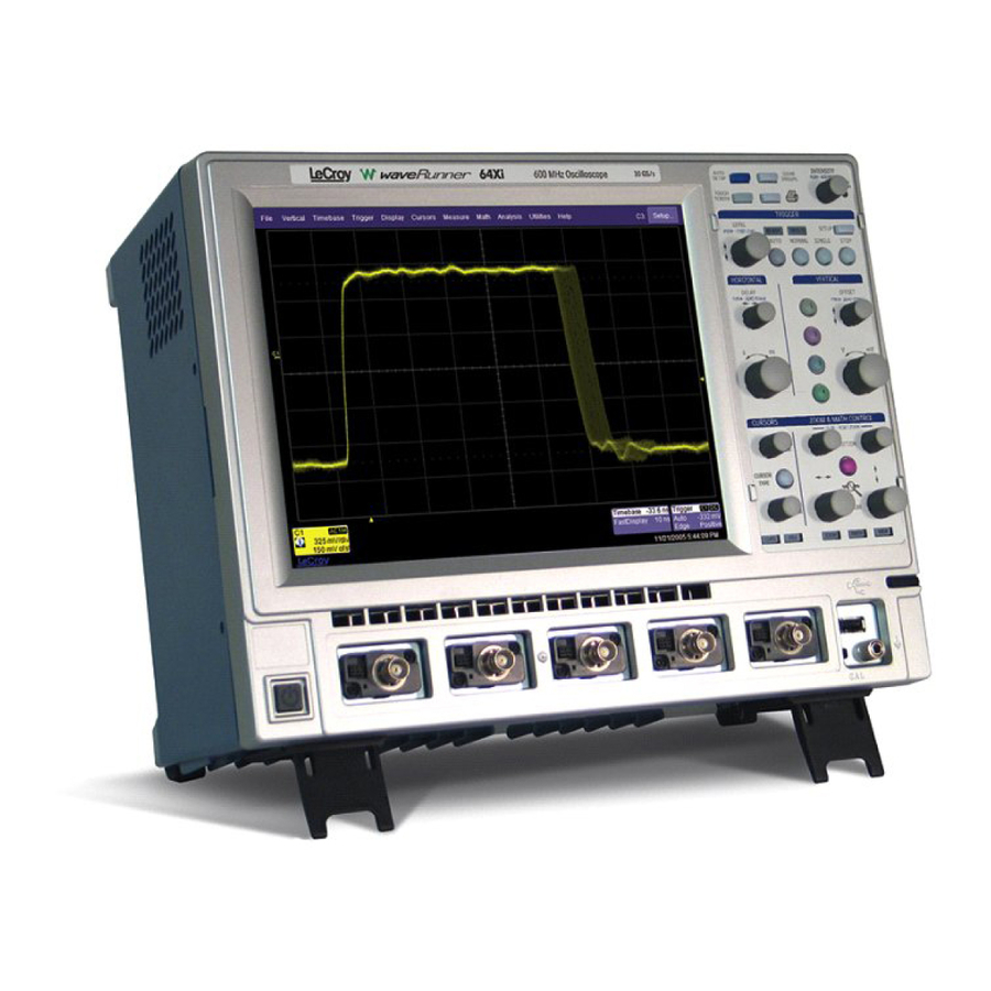
Page 1 ® UNNER I SERIES SCILLOSCOPES Operator’s Manual 2008 EBRUARY ...
Page 2 © 2008 by LeCroy Corporation. All rights reserved. LeCroy, ActiveDSO, JitterTrack, WavePro, WaveMaster, WaveSurfer, WaveLink, WaveExpert, and Waverunner are registered trademarks of LeCroy Corporation. Other product or brand names are trademarks or requested trademarks of their respective holders. Information in this publication supersedes all earlier versions.
Page 3: Table Of Contents
Warranty and Service ................................ 2 1 Environmental Characteristics ............................ 2 1 Certifications .................................. 2 1 CE Declaration of Conformity ............................ 2 1 Warranty .................................. 22 Windows License Agreement .......................... 23 End‐User License Agreement For LeCroy® X‐Stream Software ................ 23 ........................... 2 8 AFETY EQUIREMENTS Safety Symbols and Terms .............................. 2 8 Operating Environment ............................ 28 Cooling Requirements .............................. 29 AC Power Source .............................. 30 Power and Ground Connections .......................... 30 ...
Page 4 UNNER ERIES Trigger Controls .................................. 3 2 Horizontal Controls ................................ 3 2 Vertical Controls ................................. 3 3 Zoom Controls .................................. 3 3 Special Features Controls .............................. 3 3 General Control Buttons .............................. 3 4 ‐ .................. 35 SCREEN OOLBARS CONS AND IALOG ...
Page 5 ’ PERATOR ANUAL .................... 5 3 ERTICAL ETTINGS AND HANNEL ONTROLS Adjusting Sensitivity and Position .......................... 53 Sensitivity Adjustment ............................... 5 3 Adjusting the Waveform's Position ......................... 54 Coupling ................................... 54 Overload Protection ................................ 5 4 Coupling Setup ................................... 5 4 Probe Attenuation .............................. 54 Probe Attenuation Setup .............................. 5 4 Bandwidth Limit ............................... 55 Bandwidth Limiting Setup .............................. 5 5 Averaging ................................. 55 ...
Page 6 UNNER ERIES Runt Trigger .................................. 7 1 Slew Rate Trigger ................................ 7 1 .......................... 71 ISPLAY ORMATS Sequence Mode Display .............................. 7 2 Persistence Setup .............................. 72 Saturation Level ................................. 7 3 3‐Dimensional Persistence .............................. 7 3 Show Last Trace ............................... 75 Persistence Time .............................. 75 Persistence Setup .............................. 75 Screen Saver ................................ 75 Moving Traces from Grid to Grid .......................... 76 Moving a Channel or Math Trace ............................ 7 6 Zooming Waveforms ...
Page 7 ’ PERATOR ANUAL ............................ 8 7 ISTOGRAMS Creating and Viewing a Histogram ........................... 87 Single Parameter Histogram Setup ............................ 8 7 Viewing Thumbnail Histograms ............................ 8 8 Persistence Histogram ............................... 8 8 Persistence Trace Range .............................. 8 9 Persistence Sigma ................................ 8 9 Histogram Parameters ............................. 90 Histogram Theory of Operation .......................... 96 DSO Process .................................. ...
Page 8 UNNER ERIES .......................... 126 AVEFORM Introduction to Math Traces and Functions ...................... 126 Math Made Easy .............................. 126 To Set Up a Math Function ............................... 1 26 Resampling To Deskew ............................ 127 To Resample .................................. 1 27 Rescaling and Assigning Units .......................... 127 Rescaling Setup ................................ 1 29 Averaging Waveforms ............................ 129 Summed vs. Continuous Averaging .......................... 1 29 Continuous Averaging Setup ............................ 1 31 ...
Page 9 ’ PERATOR ANUAL Level Markers ................................... 1 48 Scan Overlay View .............................. 149 Scan Histogram View ............................. 150 Zoom View ................................ 151 WaveScan Search Modes ............................ 153 Edge Mode .................................. 1 53 Non‐monotonic Mode .............................. 1 54 Runt Mode .................................. 1 55 Measurement Mode ................................ 1 57 Scan Filters .................................. 1 58 WaveScan Filtering.............................. 159 ...
Page 10 UNNER ERIES Calling Excel Directly from the Instrument ........................ 1 74 Selecting a Math Function Call .......................... 174 Selecting a Parameter Function Call ........................ 174 The Excel Control Dialog ............................ 174 Entering a File Name .............................. 175 Organizing Excel sheets ............................ 175 Setting the Vertical Scale ............................ 176 Trace Descriptors .............................. 176 Multiple Inputs and Outputs .......................... 176 Examples ................................ 177 Simple Excel Example 1 .............................. 1 77 Simple Excel Example 2 .............................. 1 79 Exponential Decay Time Constant Excel Parameter (Excel Example 1) ................ 1 81 Gated Parameter Using Excel (Excel Example 2) ...................... 1 82 ...
Page 11 ’ PERATOR ANUAL Calling MATLAB from the Instrument ........................ 208 Calling MATLAB ................................ 2 08 How to Select a Waveform Function Call ...................... 209 The MATLAB Waveform Control Panel ........................ 209 MATLAB Waveform Function Editor ‐ Example ..................... 210 MATLAB Example Waveform Plot .......................... 211 How to Select a MATLAB Parameter Call ....................... 212 The MATLAB Parameter Control Panel ........................ 212 The MATLAB Parameter Editor .......................... 213 MATLAB Example Parameter Panel ........................ 213 Further Examples of MATLAB Waveform Functions .................... 214 Creating Your Own MATLAB Function ........................ 215 DSO ............................ 2 16 USTOM Custom DSO ................................ 216 Introduction – What is CustomDSO? .......................... 2 16 ...
Page 12: Introduction
Help. Returning a Product for Service or Repair If you need to return a LeCroy product, identify it by its model and serial numbers. Describe the defect or failure, and give us your name and telephone number.
Page 13: Technical Support
Within the warranty period, transportation charges to the factory will be your responsibility. Products under warranty will be returned to you with transport prepaid by LeCroy. Outside the warranty period, you will have to provide us with a purchase order number before the work can be done. You will be billed for parts and labor related to the repair work, as well as for shipping.
Page 14 UNNER ERIES • Bandwidth @ 1 Mohms (-3 dB) - typical: WaveRunner 44Xi 10 mV/div to 10 V/div 400 MHz WaveRunner 64Xi 10 mV/div to 10 V/div 500 MHz WaveRunner 62Xi 10 mV/div to 10 V/div 500 MHz 5 mV/div to 10 V/div 500 MHz WaveRunner 104MXi and WaveRunner 104Xi...
Page 15: Horizontal System
’ PERATOR ANUAL • DC Gain Accuracy: ±1.0% of full scale (typical): ±1.5% >/= 10 mV/div ±2.5% 5 mV/div ±3.5% 2 mV/div • Offset Range: ±100 µV @ 2.0 to 10 mV/div ±200 µV @ 10.1 to 20 mV/div ±500 µV @ 20.1 to 50 mV/div ±1 mV @ 51 mV to 100 mV/div ±2 mV @ 102 to 200 mV/div 50 ohms...
Page 16: Acquisition System
UNNER ERIES • Trigger & Interpolator Jitter: </= 3 ps rms (typical) • Channel-to-Channel Deskew Range: ±9 x time/div setting • Interpolator Resolution: 1.2 ps • External Sample Clock (2-channel operation only; Ch 2 only in WaveRunner 62Xi): DC to 600 MHz; 50 ohm (limited BW in 1 Mohm), BNC input, limited to 2 Ch operation (1 Ch in 62Xi), minimum rise time and amplitude requirements apply at low frequencies.
Page 17: Triggering System
’ PERATOR ANUAL • Interpolation: Linear, (sinx)/x Triggering System • Modes: Normal, Auto, Single, and Stop • Sources: Any input channel, External, Ext/10, or line; slope and level are unique to each source (except line) • Coupling Mode: GND, DC 50 ohms, DC 1 Mohms, AC 1 Mohms •...
Page 18: Automatic Setup
UNNER ERIES upper level and a lower level. Automatic Setup • Autosetup: Automatically sets timebase, trigger, and sensitivity to display a wide range of repetitive signals. • Vertical Find Scale: Automatically sets the vertical sensitivity and offset for the selected channels to display a waveform with maximum dynamic range.
Page 19: Interface
’ PERATOR ANUAL Interface • Remote Control: Through Windows® Automation or LeCroy remote command set • GPIB Port (optional): Supports IEEE-488.2 • Ethernet Port: 10/100Base-T Ethernet interface (RJ-45 connector) • USB Ports: 5 USB ports (one at front of oscilloscope) support Windows compatible devices.
Page 20: Measure Tools (Standard)
UNNER ERIES Measure Tools (standard) Display any 8 parameters together with statistics, including their average, high, low, and standard deviations. Histicons provide a fast, dynamic view of parameters and wave shape characteristics. • • amplitude mean • • area median •...
Page 21: Warranty And Service
’ PERATOR ANUAL • Power Consumption: 340 watts (340 VA) max., WaveRunner 62Xi: 290 W (290 VA), depending on accessories installed (probes, PC port plug-ins, etc.); Standby State: 12 watts • Physical Dimensions (HWD): 260 mm x 340 mm x 152 mm (10.2 in. x 13.4 in. x 6.0 in.); height measurement excludes foot pads •...
Page 22: Warranty
The instrument is warranted for normal use and operation, within specifications, for a period of three years from shipment. LeCroy will either repair or, at our option, replace any product returned to one of our authorized service centers within this period. However, in order to do this we must first examine the product and find that the defect is due to workmanship or materials and not due to misuse, neglect, accident, or abnormal conditions or operation.
Page 23: Windows License Agreement
SOIENT REDIGÉS EN LANGUE ANGLAISE. 1. GRANT OF LICENSE. 1.1 License Grant. Subject to the terms and conditions of this EULA and payment of all applicable fees, LeCroy grants to you a nonexclusive, nontransferable license (the “License”) to: (a) operate the Software Product as provided or installed, in object code form, for your own internal business purposes, (i) for use in or with an instrument provided or manufactured by LeCroy (an “Instrument”), (ii) for testing your software product(s) (to be...
Page 24 Software Product and to such acts as are necessary to achieve the Permitted Objective; (C) the information to be gained thereby has not already been made readily available to you or has not been provided by LeCroy within a reasonable time after a written request by you to LeCroy to provide such information; (D) the information gained is not used for any purpose other than the Permitted Objective and is not disclosed to any other person except as may be necessary to achieve the Permitted Objective;...
Page 25 Any Update or other supplemental software code provided to you pursuant to the Support Services will be considered part of the Software Product and will be subject to the terms and conditions of this EULA. LeCroy may use any technical information you provide to LeCroy during LeCroy’s provision of Support Services, for LeCroy’s business purposes, including for product support and development.
Page 26 BXA nor any other U.S. federal agency has suspended, revoked or denied your export privileges. It is your responsibility to comply with the latest United States export regulations, and you will defend and indemnify LeCroy from and against any damages, fines, penalties, assessments, liabilities, costs and expenses (including...
Page 27 8.5 Assignment. This EULA and the rights and obligations hereunder, may not be assigned, in whole or in part by you, except to a successor to the whole of your business, without the prior written consent of LeCroy. In the case...
Page 28: Safety Requirements
UNNER ERIES SAFETY REQUIREMENTS This section contains information and warnings that must be observed to keep the instrument operating in a correct and safe condition. You are required to follow generally accepted safety procedures in addition to the safety precautions specified in this section. Safety Symbols and Terms Where the following symbols or terms appear on the instrument’s front or rear panels, or in this manual, they alert you to important safety considerations.
Page 29: Cooling Requirements
’ PERATOR ANUAL Note: Direct sunlight, radiators, and other heat sources should be taken into account when assessing the ambient temperature. The design of the instrument has been verified to conform to EN 61010-1 safety standard per the following limits: CAUTION •...
Page 30: Ac Power Source
UNNER ERIES AC Power Source The instrument operates from a single-phase, 100 to 240 Note: The instrument automatically adapts itself (+/-10%) AC power source at 50/60 Hz (+/-5%), or to the AC line input within the following ranges: single-phase 100 to 120 V (+/-10%) AC power source at 400 Hz (+/-5%).
Page 31: Calibration
’ PERATOR ANUAL Always use the On/Standby switch to place the DSO in Standby state so that it executes a proper shutdown process (including a Windows shutdown) to preserve settings before powering itself off. This can be accomplished by pressing and holding in the On/Standby switch for approximately 5 seconds. Note: To power off, place the DSO in Standby state, then disconnect the power cord.
Page 32: Front Panel Controls
FRONT PANEL CONTROLS Front Panel Buttons and Knobs The control buttons of the WaveRunner Xi Series front panel are logically grouped into analog and special function areas. Analog functions are included in the Horizontal, Trigger, and Vertical groups of control buttons and knobs.
Page 33: Vertical Controls
’ PERATOR ANUAL Vertical Controls • - Adjusts the vertical offset of a channel. FFSET • - Adjusts the Volts/Division setting (vertical gain) of the channel selected. OLTS • HANNEL UTTONS - If the channel is already ON, the channel button makes the channel active.
Page 34: General Control Buttons
UNNER ERIES • DJUST OARSE - This dual-function knob controls the placement of the bottom or right cursor. When the knob is in Cursor mode, the CURS lamp is lit. When you click in any field in any dialog, the knob automatically switches from cursor placement mode to adjustment mode, and the ADJ lamp lights.
Page 35: On-Screen Toolbars, Icons, And Dialog Boxes
’ PERATOR ANUAL ON-SCREEN TOOLBARS, ICONS, AND DIALOG BOXES Menu Bar Buttons The menu bar buttons at the top of the oscilloscope's display are designed for quick setup of common functions. At the right end of the menu bar is a quick setup button that, when touched, opens the setup dialog associated with the trace or parameter named beside it.
Page 36: Grid Area
UNNER ERIES Grid Area The grid area contains several indicators to help you understand triggering. Indicators are coded to the channel colors (yellow here for channel 1). Trigger Delay - This indicator is located along the bottom edge of the grid. Trigger delay allows you to see the signal prior to the trigger time.
Page 37: Trace Descriptors
’ PERATOR ANUAL Trace Descriptors Vertical and horizontal trace descriptor labels are displayed below the grid. They provide a summary of your channel, timebase, and trigger settings. To make adjustments to these settings, touch the respective label to display the setup dialog for that function. Channel trace labels show the vertical settings for the trace, as well as cursor information if cursors are in use.
Page 38: Dialog Boxes
UNNER ERIES Dialog Boxes The dialog area occupies the bottom one-third of the screen. To expand the signal display area, you can minimize each dialog box by touching the Close tab at the right of the dialog box. Alternate Access Methods The instrument often gives you more than one way to access dialogs and menus.
Page 39: Trace Annotation
’ PERATOR ANUAL Trace Annotation The instrument gives you the ability to add an identifying label, bearing your own text, to a waveform display: For each waveform, you can create multiple labels and turn them all on or all off. Also, you can position them on the waveform by dragging or by specifying an exact horizontal position.
Page 40 UNNER ERIES • You may place a label anywhere you want on the waveform. Labels are numbered sequentially according to the order in which they are added, and not according to their placement on the waveform. WRXi-OM-E Rev B...
Page 41: To Turn On A Channel Trace Label
’ PERATOR ANUAL • If you want to change the label's text, touch inside the Label Text field. A pop-up keyboard appears for you to enter your text. Touch O.K. on the keyboard when you are done. Your edited text will automatically appear in the label on the waveform.
Page 42: Hardware Connections
1. In the menu bar, touch Utilities. 2. In the dialog area, touch Status. Adding a New Option To add a software option you will need a code to enable the option. Call LeCroy Customer Support to place an order and receive the code. Restoring Software Restarting the Application Upon initial power-up, the oscilloscope will load the instrument application software automatically.
Page 43: Monitor Hookup
’ PERATOR ANUAL Monitor Hookup 1. Connect the external monitor to the VGA port on the side of the instrument (item 4). 2. Plug in the monitor's power cord, and apply power to the monitor. Video Setup After boot-up, configure the monitors as follows: Note: A mouse is required for dual monitor use.
Page 44: Default Settings
3. Then touch the on-screen Recall Default button. Adding a New Option To add a software option you need a key code to enable the option. Call LeCroy Customer Support to place an order and receive the code. Add the software option by doing the following: 1.
Page 45: Restoring Software
CONNECTING TO A SIGNAL ProBus Interface LeCroy's ProBus probe system provides a complete measurement solution from probe tip to oscilloscope display. ProBus allows you to control transparent gain and offset directly from your front panel. It is particularly useful for voltage, differential, and current active probes.
Page 46: Auxiliary Output Setup
LeCroy as optional accessories. The PP008 is designed for use with 600 MHz and lower LeCroy WaveRunner Xi series oscilloscopes. Refer to the PP008 Instruction Manual. LeCroy also offers a variety of passive and active probes for use with your WaveRunner Xi Series oscilloscope.
Page 47 ’ PERATOR ANUAL Probes WRXi-OM-E Rev B...
Page 48: Probe Compensation
UNNER ERIES Probe Compensation Passive probes must be compensated to flatten overshoot. This is accomplished by means of a trimmer at the connector end of the probe. 1. Attach the connector end of your PP008 probe to any channel. 2. Connect the probe end to the CAL output connector at the front of the oscilloscope. 3.
Page 49: Selecting A Sampling Mode
’ PERATOR ANUAL Selecting a Sampling Mode 1. In the menu bar, touch Timebase, then Horizontal Setup... in the drop-down menu. 2. In the Horizontal dialog, touch a Sample Mode button. 3. If you chose Sequence Mode, touch the Smart Memory tab, then touch inside the Num Segments field and enter a value using the pop-up numeric keypad.
Page 50: Sequence Mode Setup
UNNER ERIES Each individual segment can be zoomed or used as input to math functions. The instrument uses the sequence timebase setting to determine the capture duration of each segment: 10 x time/div. Along with this setting, the oscilloscope uses the desired number of segments, maximum segment length, and total available memory to determine the actual number of samples or segments, and time or points.
Page 51: Sequence Display Modes
’ PERATOR ANUAL Sequence Display Modes The instrument gives you a choice of five ways to display your segments: DJACENT ATERFALL CASCADED OSAIC TILED VERLAY ERSPECTIVE The number of segments you choose to display (80 maximum) can be less than the total number of segments in the waveform.
Page 52: Displaying Individual Segments
UNNER ERIES Displaying Individual Segments 1. Touch Math in the menu bar, then Math Setup... in the drop-down menu. 2. Touch a function tab (F1 to Fx The number of math traces available depends on the software options loaded on your oscilloscope. See specifications.). 3.
Page 53: Roll Mode
’ PERATOR ANUAL Roll Mode • Roll mode can be selected when the timebase mode is real time, time per division is > 200 ms/div, and the sampling rate is < 200 kS/s. • Roll mode is not selected automatically when the above criteria are met. You must select Roll mode manually from the Timebase dialog each time you want to invoke it.
Page 54: Adjusting The Waveform's Position
2. Touch inside the Coupling field and select a coupling mode from the pop-up menu. Probe Attenuation Probe Attenuation Setup LeCroy's ProBus system automatically senses probes and sets their attenuation for you. However, to set the attenuation manually: 1. In the menu bar, touch Vertical, then select a channel from the drop-down menu.
Page 55: Bandwidth Limit
’ PERATOR ANUAL Bandwidth Limit Reducing the bandwidth also reduces the signal and system noise, and prevents high frequency aliasing. Bandwidth Limiting Setup To set bandwidth limiting: 1. In the menu bar, touch Vertical, then select a channel from the drop-down menu. 2.
Page 56: Variable Gain
UNNER ERIES Variable Gain Variable Gain lets you change the granularity with which the gain is incremented. For example, when Variable Gain is disabled, the gain will increase or decrease in preset increments of 10 or 100 mV each time you touch the Up/Down buttons.
Page 57: Combining Channels
’ PERATOR ANUAL Refer to Acquisition Modes in the specifications for maximum sample rates. Combining Channels 1. In the menu bar, touch Timebase, then Horizontal Setup... in the drop-down menu. 2. Under “Active Channels,” touch 4, 2, or Auto. The maximum sample rate is shown alongside each button. Autosetup When channels are turned on, Autosetup operates only on those turned-on channels.
Page 58 UNNER ERIES State The State trigger is a level-qualified trigger which requires that the qualifying signal remain above or below a specified voltage level for a trigger to occur. For Sate trigger, you specify the time or number of events after the signal has gone above or below the voltage level when you want the trigger to occur.
Page 59: Determining Trigger Level, Slope, Source, And Coupling
’ PERATOR ANUAL Determining Trigger Level, Slope, Source, and Coupling 1. Level defines the source voltage at which the trigger circuit will generate an event: a change in the input signal that satisfies the trigger conditions. The selected trigger level is associated with the chosen trigger source.
Page 60: Level
UNNER ERIES Level Level defines the source voltage at which the trigger circuit will generate an event (a change in the input signal that satisfies the trigger conditions). The selected trigger level is associated with the chosen trigger source. Note that the trigger level is specified in volts and normally remains unchanged when the vertical gain or offset is modified.
Page 61: Hold Off By Events
’ PERATOR ANUAL Hold Off by Events Select a positive or negative slope and a number of events. An event is the number of times the trigger condition is met after the last trigger. A trigger is generated when the condition is met after this number, counted from the last trigger.
Page 62: Edge Trigger Setup
UNNER ERIES Alternatively, in the Trigger dialog, you can touch inside the Level field and type in a value, using the pop-up numeric keypad. To quickly set a level of zero volts, touch the Zero Level button directly below the Coupling field.
Page 63: Width Trigger
’ PERATOR ANUAL 9. Choose Positive, Negative, or Window slope. Window slope sets a threshold above and below the trigger level beyond which the signal must pass to generate a trigger. The slope can be either positive or negative. Width Trigger IDTH RIGGER ORKS...
Page 64: Qualified Trigger
UNNER ERIES Qualified Trigger UALIFIED RIGGERS Use a signals transition above or below a given level (its validation) as an enabling (qualifying) condition for a second signal that is the trigger source. These are Qualified triggers. For Edge Qualified triggers (the default) the transition is sufficient and no additional requirement is placed on the first signal.
Page 65: Pattern (Logic) Trigger
’ PERATOR ANUAL UALIFIED RIGGER ETUP 1. Touch the Trigger descriptor label. 2. Touch the Qualified trigger button. 3. Under "Arm trigger on Event 'A'" select Edge as the condition on which to arm the trigger. The Edge condition will automatically be selected under "Then trigger on Event 'B'" also. 4.
Page 66: Tv Trigger
UNNER ERIES 4. If applicable, touch the Pattern tab. For each input you want to include in the logic pattern, touch inside the State field and select a logic state: Low or High. Select Don't Care for all other inputs. 5.
Page 67: Smart Triggers
’ PERATOR ANUAL USTOM RIGGER ETUP 1. Touch the Custom button to select Custom mode. 2. Touch inside # of Lines, and enter a value up to 1500, using the pop-up keypad. 3. Touch inside Hz and select 50 or 60 Hz from the pop-up menu. 4.
Page 68: Interval Trigger
UNNER ERIES LITCH RIGGER ETUP 1. Touch the Trigger descriptor label. 2. If applicable, touch the Smart trigger button, then the Glitch trigger button. 3. Touch inside the trigger Source field and select a source on which to trigger. 4. Touch inside the Level data entry field and enter a value using the pop-up keypad. 5.
Page 69 ’ PERATOR ANUAL Interval Trigger that triggers when the interval width is larger than the set interval. The broken upward-pointing arrow indicates a potential trigger, while the bold one shows where the actual trigger occurs on the positive edge after the selected interval. •...
Page 70: Dropout Trigger
UNNER ERIES NTERVAL RIGGER ETUP 1. Touch the Trigger descriptor label. 2. If applicable, touch the Smart trigger button, then the Interval trigger button. 3. Touch inside the Trigger Source field and select a source on which to trigger. 4. If available, touch inside the Coupling field and select a coupling mode. 5.
Page 71: Runt Trigger
’ PERATOR ANUAL Runt Trigger The Runt trigger is programmed to occur when a pulse crosses a first threshold line and fails to cross a second threshold line before recrossing the first. You can select both voltage thresholds within a time range of 100 ps to 20 s.
Page 72: Sequence Mode Display
UNNER ERIES 3. Touch inside the Grid Intensity field and enter a value from 0 to 100 using the pop-up keypad. 4. Touch the Grid on Top checkbox if you want to superimpose the grid over the waveform. Depending on the grid intensity, some of your waveform may be hidden from view when the grid is placed on top.
Page 73: Saturation Level
’ PERATOR ANUAL Saturation Level The Persistence display is generated by repeated sampling of the amplitudes of events over time, and the accumulation of the sampled data into "3-dimensional" display maps. These maps create an analog-style display. User-definable persistence duration can be used to view how the maps evolve proportionally over time. Statistical integrity is preserved because the duration (decay) is proportional to the persistence population for each amplitude or time combination in the data.
Page 74 UNNER ERIES Here is an example of a 3-dimensional view of a square wave using the solid view of color-graded persistence. Saturation is set at 50%, with red areas indicating highest intensity. The X-axis has been rotated 60%; the Y-axis has been rotated 15%. Here is a monochrome (analog) view of the same waveform.
Page 75: Show Last Trace
’ PERATOR ANUAL Show Last Trace For most applications, you may not want to show the last trace because it will be superimposed on top of your persistence display. In those cases turn off Show Last Trace by touching the checkbox. However, if you are doing mask testing and want to see where the last trace is falling, turn Show Last Trace on.
Page 76: Moving Traces From Grid To Grid
UNNER ERIES Moving Traces from Grid to Grid You can move traces from grid to grid at the touch of a button. Moving a Channel or Math Trace 1. Touch the descriptor label for the waveform that you want to move. 8.
Page 77: Zooming A Single Channel
’ PERATOR ANUAL When you zoom a waveform, an approximation of the zoomed area will appear in a thumbnail icon in the Vertical Adjust dialog: Zooming a Single Channel 1. In the menu bar, touch Vertical; then touch a channel number in the drop-down menu. Alternatively, you can just touch the channel trace label for a displayed channel.
Page 78: Quickly Zooming Multiple Waveforms
UNNER ERIES 3. To set precise horizontal or vertical zoom factors, touch inside the appropriate S CALE field and enter a time-per-div value, using the pop-up numeric keypad. Turn the front panel zoom P OSITION knobs to adjust the vertical and horizontal position of the zoom. Turn the front panel Z knobs to control the boundaries of the zoom.
Page 79: Xy Display
’ PERATOR ANUAL 6. Use the Auto-Scroll buttons at the right of the Multi-Zoom dialog to control the zoomed section of your waveforms: URNING ULTI 1. In the menu bar, touch Math, then Math Setup... in the drop-down menu. 2. Touch the Multi-Zoom On checkbox to turn off Multi-zoom: XY Display Use XY displays to measure the phase shift between otherwise identical signals.
Page 80: Saving Oscilloscope Settings
UNNER ERIES Saving Oscilloscope Settings 1. In the menu bar, touch File; then touch Save Setup... in the drop-down menu. Or, press the Save/Recall front panel button, then touch the Save Setup tab. 2. To Save To File, touch inside the Save Instrument Settings field and use the pop-up keyboard to enter the path to the destination folder.
Page 81: Saving And Recalling Waveforms
’ PERATOR ANUAL Saving and Recalling Waveforms Saving Waveforms 1. In the menu bar, touch File; then touch Save Waveform... in the drop-down menu. 2. In the Save Waveform dialog, touch the Save To button. 3. Touch inside the Source field and select a source from the pop-up menu. The source can be any trace; for example, a channel (C1-C4), math function (F1-F4), or a waveform stored in memory (M1-M4).
Page 82: Recalling Waveforms
UNNER ERIES You can also enable Auto Save from this dialog by touching one of the Auto Save buttons : Wrap (old files overwritten) or Fill (no files overwritten). CAUTION If you select Fill, you can quickly use up all disk space on your hard disk. Recalling Waveforms 1.
Page 83: Deleting All Files In A Folder
’ PERATOR ANUAL Deleting All Files in a Folder 1. Touch File in the menu bar, then Disk Utilities... in the drop-down menu. 2. Touch the Delete button in the Disk Utilities dialog. 3. Touch inside the Current folder field and use the pop-up keyboard to enter the path to the folder that contains the file you want to delete.
Page 84: Adding Printers And Drivers
UNNER ERIES Adding Printers and Drivers Note: If you want to add a printer driver, the driver must first be loaded on the oscilloscope. 1. In the menu bar, touch File, then Print Setup... in the drop-down menu. The Utilities Hardcopy dialog opens. 2.
Page 85: Windows Setups
Please follow these recommendations: • Do not load any version of Windows not provided by LeCroy. If you load any Windows 2000 service packs from Microsoft, please be advised that LeCroy cannot guarantee trouble-free operation afterwards.
Page 86: Windows Repair Disk
ERIES Windows Repair Disk Before you install any hardware or software on your instrument, LeCroy strongly recommends that you create an Emergency Repair Disk. During a system rebuild, the repair process relies on information that is saved in the systemroot\repair folder. You must not change or delete this folder.
Page 87: Histograms
’ PERATOR ANUAL 4. Touch inside the Source1 field and select an input waveform from the pop-up menu. 5. Touch inside the Measure field and select a parameter from the pop-up menu. 6. Touch the Track button at the bottom of the dialog; then, from the Math selection for Track menu, select a math function location (F1 to Fx The number of math traces available depends on the software options loaded on your oscilloscope.
Page 88: Viewing Thumbnail Histograms
UNNER ERIES 9. In the dialog to the right, touch the Histogram tab. 10. Under "Buffer," touch inside the #Values field and enter a value. 11. Under "Scaling," touch inside the #Bins field and enter a value from 20 to 2000. 12.
Page 89: Persistence Trace Range
’ PERATOR ANUAL ERSISTENCE ISTOGRAM ETUP 1. In the menu bar, touch Math, then Math Setup. 2. Touch one of function tabs F1 through Fx The number of math traces available depends on the software options loaded on your oscilloscope. See specifications.. 3.
Page 90: Histogram Parameters
UNNER ERIES Histogram Parameters fwhm Full Width at Half Maximum Definition: Determines the width of the largest area peak, measured between bins on either side of the highest bin in the peak that have a population of half the highest's population. If several peaks have an area equal to the maximum population, the leftmost peak is used in the computation.
Page 91 ’ PERATOR ANUAL hist ampl Histogram Amplitude Definition: The difference in value of the two most populated peaks in a histogram. This parameter is useful for waveforms with two primary parameter values, such as TTL voltages, where hampl would indicate the difference between the binary `1' and `0' voltage values. Description: The values at the center (line dividing the population of peak in half) of the two highest peaks are determined (see pks parameter description:).
Page 92 UNNER ERIES hist maxp Histogram Maximum Population Definition: The count (vertical value) of the highest population bin in a histogram. Description: Each bin between the parameter cursors is examined for its count. The highest count is returned as maxp. Example: Here, maxp is 14. hist mode ...
Page 93 ’ PERATOR ANUAL hist rms Histogram Root Mean Square Definition: The rms value of the values in a histogram. Description: The center value of each populated bin is squared and multiplied by the population (height) of the bin. All results are summed and the total is divided by the population of all the bins. The square root of the result is returned as hrms.
Page 94 UNNER ERIES pctl Percentile Definition: Computes the horizontal data value that separates the data in a histogram such that the population on the left is a specified percentage `xx' of the total population. When the threshold is set to 50%, pctl is the same as hmedian. Description: The total population of the histogram is determined.
Page 95 ’ PERATOR ANUAL Example: Here the two peaks have been identified. The peak with the highest population is peak #1. totp Total Population Definition: Calculates the total population of a histogram between the parameter cursors. Description: The count for all populated bins between the parameter cursors is summed. Example: The total population of this histogram is 9.
Page 96: Histogram Theory Of Operation
UNNER ERIES Histogram Theory of Operation An understanding of statistical variations in parameter values is needed for many waveform parameter measurements. Knowledge of the average, minimum, maximum, and standard deviation of the parameter may often be enough, but in many cases you may need a more detailed understanding of the distribution of a parameter's values.
Page 97: Parameter Buffer
’ PERATOR ANUAL Some of these are pre-defined but can be changed. Once they are defined, the oscilloscope is ready to make the histogram. The sequence for acquiring histogram data is as follows: 1. Trigger 2. Waveform acquisition 3. Parameter calculations 4.
Page 98: Histogram Peaks
UNNER ERIES Histogram parameters are provided to enable these measurements. Available through selecting Statistics from the Category menu, they are calculated for the selected section between the parameter cursors: • fwhm - full width (of largest peak) at half the maximum bin •...
Page 99: Binning And Measurement Accuracy
’ PERATOR ANUAL However, signal noise and the use of a high number of bins relative to the number of parameter values acquired, can give a jagged and spiky histogram, making meaningful peaks hard to distinguish. The oscilloscope analyzes histogram data to identify peaks from background noise and histogram definition artifacts such as small gaps, which are due to very narrow bins.
Page 100: Cursors Setup
UNNER ERIES Cursors Setup Quick Display At any time, you can change the display of cursor types (or turn them off) without invoking the Cursors Setup dialog as follows: 1. In the menu bar, touch Cursors, then Off, Abs Horizontal, Rel Horizontal, Abs Vertical, or Rel Vertical. 2.
Page 101: Status Symbols
’ PERATOR ANUAL Status Symbols Below each parameter appears a symbol that indicates the status of the parameter, as follows: A green check mark means that the oscilloscope is returning a valid value. A crossed-out pulse means that the oscilloscope is unable to determine top and base; however, the measurement could still be valid.
Page 102: Statistics
UNNER ERIES 4. Select Measure Parameter in error (P1) Out Result 5. Read the status information in line StatusDescription. Statistics By touching the Statistics On checkbox in the Measure, you can display statistics for standard vertical or horizontal parameters, or for custom parameters. The statistics that are displayed are as follows: value (last) mean min.
Page 103: Standard Vertical Parameters
’ PERATOR ANUAL Standard Vertical Parameters These are the default Standard Vertical Parameters: Vertical mean sdev max. min. ampl pkpk base Standard Horizontal Parameters These are the default Standard Horizontal Parameters: Horizontal freq period width rise fall delay duty npoints My Measure You can choose to customize up to eight parameters by touching My Measure.
Page 104: Parameter Script Parameter Math
UNNER ERIES Parameter Script Parameter Math In addition to the arithmetic operations, the Parameter Math feature allows you to use VBScript or JavaScript to write your own script for one or two measurements and produce a result that suits your needs. Code entry is done in the Script Editor window directly on the instrument.
Page 105: Parameter Math Setup
’ PERATOR ANUAL The inputs to Param Script can also be math (F1-Fx) or memory (M1-Mx) traces. The inputs to P Script can be the results of any parameter measurement, not necessarily Param Script. Parameter Math Setup 1. Touch Measure in the menu bar, then Measure Setup... in the drop-down menu. 2.
Page 106: Measure Gate
UNNER ERIES Measure Gate Using Measure Gate, you can narrow the span of the waveform on which to perform parameter measurements, allowing you to focus on the area of greatest interest. You have the option of dragging the gate posts horizontally along the waveform, or specifying a position down to hundredths of a division.
Page 107: Help Markers
’ PERATOR ANUAL 3. Touch inside the Start field and enter a value, using the pop-up numeric keypad. Or, you can simply touch the leftmost grid line and drag the gate post to the right. 4. Touch inside the Stop field and enter a value, using the pop-up numeric keypad. Or, you can simply touch the rightmost grid line and drag the gate post to the left.
Page 108: Setting Up Help Markers
UNNER ERIES Setting Up Help Markers 1. In the menu bar, touch Measure Setup... 2. Select a Measure Mode: Std Vertical, Std Horizontal, or My Measure. 3. Touch the Show All button to display Help Markers for every parameter being measured on the displayed waveform (C2 in the examples above).
Page 109: From A Vertical Setup Dialog
’ PERATOR ANUAL From a Vertical Setup Dialog 1. In the Cx Vertical Adjust dialog, touch the Measure button 2. Select a parameter from the pop-up menu. (The Actions for trace source defaults to the channel or trace whose dialog is open. If a parameter, it goes into the next "available" parameter, or the last one if all are used.) 3.
Page 110: Determining Time Parameters
UNNER ERIES ETERMINING ISE AND IMES Once top and base are estimated, calculation of the rise and fall times is easily done (see Figure 1). The 90% and 10% threshold levels are automatically determined by the DDA-5005, using the amplitude (ampl) parameter. Threshold levels for rise or fall time can also be selected using absolute or relative settings (r@level, f@level).
Page 111: Determining Differential Time Measurements
’ PERATOR ANUAL Determining Differential Time Measurements The DDA-5005 enables accurate differential time measurements between two traces: for example, propagation, setup and hold delays (see Figure 3). Parameters such as Delta c2d± require the transition polarity of the clock and data signals to be specified. Figure 3 Moreover, a hysteresis range may be specified to ignore any spurious transition that does not exceed the boundaries of the hysteresis interval.
Page 112 UNNER ERIES Parameter Description Definition Notes Base Lower of two most probable states Value of most On signals not having two major (higher is top). Measures lower level in probable lower state levels (triangle or saw-tooth two-level signals. Differs from min in waves, for example), returns same that noise, overshoot, undershoot, and value as min.
Page 113 ’ PERATOR ANUAL Parameter Description Definition Notes Delta delay delay: Computes time between Time between midpoint Standard parameter. 50% level of two sources. transition of two sources Dperiod@level Adjacent cycle deviation (cycle-to- Reference levels and edge- cycle jitter) of each cycle in a transition polarity can be waveform selected.
Page 114 UNNER ERIES Parameter Description Definition Notes Edge@level Number of edges in waveform. Reference levels and edge- transition polarity can be selected. Hysteresis argument used to discriminate levels from noise in data. Available with JTA2 and XMAP options. Excel Performs measurements in Excel Available with XMAP option.
Page 115 ’ PERATOR ANUAL Parameter Description Definition Notes Frequency Frequency: Period of cyclic 1/period Standard parameter. signal measured as time between every other pair of 50% crossings. Starting with first transition after left cursor, the period is measured for each transition pair. Values then averaged and reciprocal used to give frequency.
Page 116 UNNER ERIES Parameter Description Definition Notes Hist median Value of the "X" axis of a Available with DDM2, JTA2, histogram that divides the and XMAP options. population into two equal Standard in DDA-5005A. halves. Hist minimum Value of the lowest (left-most) Available with DDM2, JTA2, populated bin in a histogram.
Page 117 ’ PERATOR ANUAL Parameter Description Definition Notes Local bsep Local baseline separation, Hysteresis argument used to between rising and falling discriminate levels from noise slopes. in data. Available with DDM2 option. Standard in DDA-5005A. Local max Maximum value of a local Hysteresis argument used to feature.
Page 118 UNNER ERIES Local tmax Time of the maximum value of Hysteresis argument used to a local feature. discriminate levels from noise in data. Available with DDM2 option. Standard in DDA-5005A. Local tmin Time of the minimum value of a Hysteresis argument used to local feature.
Page 119 ’ PERATOR ANUAL Parameter Description Definition Notes Maximum Measures highest point in Highest value in waveform Gives similar result when waveform. Unlike top, does not between cursors applied to time domain assume waveform has two waveform or histogram of data levels.
Page 120 UNNER ERIES Parameter Description Definition Notes N-cycle jitter Peak-to-peak jitter between Compares the expected time Available in SDA analyzers. edges spaced n UI apart. to the actual time of leading edges n bits apart. NLTS Provides a measurement of the Available with DDM2 option.
Page 121 ’ PERATOR ANUAL Parameter Description Definition Notes Period Period of a cyclic signal Where: Mr is the number of measured as time between leading edges found, Mf the every other pair of 50% number of trailing edges crossings. Starting with first transition after left cursor, found, the time when...
Page 122 UNNER ERIES Parameter Description Definition Notes Range Calculates range (max min) of Available with DDM2, JTA2, a histogram. and XMAP options. Standard in DDA-5005A. Resolution Ratio of taa for a high and low taa (HF)/mean taa (LF)*100 Hysteresis argument used to frequency waveform discriminate levels from noise in data.
Page 123 ’ PERATOR ANUAL Parameter Description Definition Notes Root Mean Square of data Gives similar result when between the cursors - about applied to time domain same as sdev for a zero-mean waveform or histogram of data waveform. of same waveform. But with histograms, result may include contributions from more than one acquisition.
Page 124 UNNER ERIES Parameter Description Definition Notes Average peak-to-trough Hysteresis argument used to amplitude for all local features. discriminate levels from noise in data. Available with DDM2 option. Standard in DDA-5005A. TAA- Average local baseline-to- Hysteresis argument used to trough amplitude for all local discriminate levels from noise features.
Page 125 ’ PERATOR ANUAL Parameter Description Definition Notes Higher of two most probable Value of most probable Gives similar result when states, the lower being base; it higher state applied to time domain is characteristic of rectangular waveform or histogram of data waveforms and represents the of same waveform.
Page 126: Introduction To Math Traces And Functions
UNNER ERIES WAVEFORM MATH Introduction to Math Traces and Functions With the instrument’s math tools you can perform mathematical functions on a waveform displayed on any channel, or recalled from any of the four reference memories M1 to M4. You can also set up traces F1 to Fx The number of math functions that can be performed at the same time depends on the software options loaded on your oscilloscope.
Page 127: Resampling To Deskew
’ PERATOR ANUAL Histogram of the values of a parameter Track of the values of a parameter Trend of the values of a parameter Resampling To Deskew Deskew whenever you need to compensate for different lengths of cables, probes, or anything else that might cause timing mismatches between signals.
Page 128 UNNER ERIES Hertz Joule Degree Kelvin Degree Celsius Degree Fahrenheit Liter Meter Foot Inch YARD yard MILE mile Newton Pascal Percent POISE Poise parts per million Radian Degree (of arc) Minute (of arc) SAMPLE sample SWEEP sweeps Second (of arc) Second Siemens Tesla...
Page 129: Rescaling Setup
’ PERATOR ANUAL You can also enter combinations of the previous units following the SI rules: • for the quotient of two units, the character / should be used • for the product of two units, the character . should be used •...
Page 130 UNNER ERIES UMMED VERAGING Summed Averaging is the repeated addition, with equal weight, of successive source waveform records. If a stable trigger is available, the resulting average has a random noise component lower than that of a single-shot record. Whenever the maximum number of sweeps is reached, the averaging process stops. An even larger number of records can be accumulated simply by changing the number in the dialog.
Page 131: Continuous Averaging Setup
’ PERATOR ANUAL Continuous Averaging Setup 1. In the menu bar, touch Math, then Math Setup... in the drop-down menu. 2. Select a function tab from F1 through Fx The number of math traces available depends on the software options loaded on your oscilloscope. See Specifications.. 3.
Page 132 UNNER ERIES With low-pass filters, the actual SNR increase obtained in any particular situation depends on the power spectral density of the noise on the signal. The improvement in SNR corresponds to the improvement in resolution if the noise in the signal is white - evenly distributed across the frequency spectrum.
Page 133 ’ PERATOR ANUAL The following examples illustrate how you might use the instrument's enhanced resolution function. In low-pass filtering: The spectrum of a square signal before (left top) and after (left bottom) enhanced resolution processing. The result clearly illustrates how the filter rejects high-frequency components from the signal. The higher the bit enhancement, the lower the resulting bandwidth.
Page 134: Enhanced Resolution (Eres) Setup
UNNER ERIES Enhanced Resolution (ERES) Setup 1. In the menu bar, touch Math, then Math Setup... in the drop-down menu. 2. Touch a function tab F1 through Fx The number of math traces available depends on the software options loaded on your oscilloscope. See Specifications.. 3.
Page 135: Waveform Sparser Setup
’ PERATOR ANUAL Waveform Sparser Setup 1. In the menu bar, touch Math, then Math setup... in the drop-down menu. 2. Touch the tab for the function (F1 to Fx The number of math traces available depends on the software options loaded on your oscilloscope.
Page 136: Power (Density) Spectrum
This variation in spectrum magnitude is the picket fence effect. The corresponding attenuation loss is referred to as scallop loss. LeCroy oscilloscopes automatically correct for the scallop effect, ensuring that the magnitude of the spectra lines correspond to their true values in the time domain.
Page 137: Improving Dynamic Range
The SNR increase is conditioned by the cut-off frequency of the ERES low-pass filter and the noise shape (frequency distribution). LeCroy digital oscilloscopes employ FIR digital filters so that a constant phase shift is maintained. The phase information is therefore not distorted by the filtering action.
Page 138: Fft Algorithms
UNNER ERIES An effective way to reduce these effects is to maximize the acquisition record length. Record length directly conditions the effective sampling rate of the oscilloscope and therefore determines the frequency resolution and span at which spectral analysis can be carried out. FFT Algorithms A summary of the algorithms used in the oscilloscope's FFT computation is given here in a few steps: The data are multiplied by the selected window function.
Page 139: Fft Glossary
’ PERATOR ANUAL where M = 0.316 V (that is, 0 dBm is defined as a sine wave of 0.316 V peak or 0.224 V rms, giving 1.0 mW into 50 ohms). The dBm Power Spectrum is the same as dBm Magnitude, as suggested in the above formula. dBm Power Density: where ENBW is the equivalent noise bandwidth of the filter corresponding to the selected window, and Delta f is the current frequency resolution (bin width).
Page 140 UNNER ERIES For a real source waveform (imaginary part equals 0), there are only N/2 independent harmonic components. An FFT corresponds to analyzing the input signal with a bank of N/2 filters, all having the same shape and width, and centered at N/2 discrete frequencies. Each filter collects the signal energy that falls into the immediate neighborhood of its center frequency.
Page 141: Fft Setup
’ PERATOR ANUAL Power Density Spectrum The power density spectrum (V /Hz) is the power spectrum divided by the equivalent noise bandwidth of the filter, in hertz. The power density spectrum is displayed on the dBm scale, with 0 dBm corresponding to (V /Hz).
Page 142: Analysis
UNNER ERIES 7. Choose whether to Truncate or Zero-fill the trace display. 8. Touch the Suppress DC checkbox if you want to make the DC bin go to zero. Otherwise, leave it unchecked. 9. Touch inside the Output type field, and make a selection from the pop-up menu. 10.
Page 143: Mask Tests
’ PERATOR ANUAL In Dual Parameter Compare mode, your X-Stream oscilloscope gives you the option to compare to each other parameter results measured on two different waveforms. You can set your test to be true if Any waveform or All waveforms fit the criterion stipulated by the comparison condition.
Page 144: Setting Up Pass/Fail Testing
UNNER ERIES Setting Up Pass/Fail Testing Initial Setup 1. Touch Analysis in the menu bar, then Pass/Fail Setup... in the drop-down menu. 2. Touch the Actions tab. 3. Touch the Enable Actions checkbox. This will cause the actions that you will select to occur upon your waveform's passing or failing a test.
Page 145: Comparing Dual Parameters
’ PERATOR ANUAL 6. Touch inside the Condition field in the ParamCompare mini-dialog and select a math operator from the pop- up menu: 7. Touch inside the Limit field and enter a value, using the pop-up numeric keypad. This value takes the dimensions of the parameter that you are testing.
Page 146: Mask Testing
UNNER ERIES 7. Touch inside the Condition field in the ParamCompare mini-dialog and select a math operator from the pop- up menu: 8. Touch inside the Limit field and enter a value, using the pop-up numeric keypad. This value takes the dimension of the parameter that you are testing.
Page 147: Wavescan
’ PERATOR ANUAL WAVESCAN Introduction to WaveScan WaveScan enables you to search for unusual events in a single capture, or to scan for an event in many acquisitions over a long period of time. You can select from more than 20 search modes (frequency, rise time, runt, duty cycle, etc.), apply a search condition (slope, level, threshold, hysteresis), and begin scanning in a post- acquisition environment.
Page 148: Search Modes
UNNER ERIES Search Modes Search modes are used to locate anomalies during acquisition. • Edge - for detecting the occurrence of edges; selectable slope and level • Non-monotonic - for detecting threshold re-crosses; selectable slope, hysteresis, and level • Runt - for detecting pulses that fail to cross a threshold; selectable polarity and thresholds •...
Page 149: Scan Overlay View
’ PERATOR ANUAL Scan Overlay View This display mode shows all edges in an acquisition overlaid one on top of the other. By default, monochromatic persistence is turned on for the scan overlays, but you have the option to disable it. Saturation and persistence time controls are also available.
Page 150: Scan Histogram View
UNNER ERIES Scan Histogram View By enabling ScanHisto, a histogram corresponding to your search criteria is superimposed on the overlay trace. In the example below, the Rise 10-90% parameter measurement has been applied, but only edges slower than 1.2 ns with a delta of 50 ps are accumulated in the histogram. Another feature of WaveScan is that you can select a single bin of the histogram for analysis by touching or clicking it.
Page 151: Zoom View
’ PERATOR ANUAL Zoom View An individual edge can be zoomed by selecting it from the table of found events at the left of the screen. You can also scroll through the table using the Prev/Next scroll buttons in the Search dialog, or select an event by touching inside the Idx field and entering an index number, using the pop-up keypad.
Page 152 UNNER ERIES When the Idx field is active, or when an edge is selected in the table, you can use the front panel A DJUST knob to advance through the table contents, one line at a time. When the table contents are too numerous to fit in a single table display, a scroll bar will appear. By touching the scroll bar to highlight it, you can use the Adjust knob to quickly scroll through the table.
Page 153: Wavescan Search Modes
’ PERATOR ANUAL WaveScan Search Modes Edge Mode This search mode locates all edges in an acquisition and presents them time-stamped in a table. You can select positive, negative, or both edges. When the acquisition is stopped, scan filters contained in Measurements mode can be applied to the edges to find specific characteristics.
Page 154: Non-Monotonic Mode
UNNER ERIES Non-monotonic Mode The Non-monotonic search mode looks for edges that cross a threshold more than once between high and low levels. All events that meet the criteria of slope, hysteresis, and level are presented in a table and highlighted in the source trace.
Page 155: Runt Mode
’ PERATOR ANUAL Runt Mode This search mode looks for pulses that fail to transit a given region. You can search for positive-going or negative- going runts, or both. An adjustable hysteresis band is provided to eliminate noise. In the case of negative-going runt pulses, the value displayed in the table is the difference (delta) of the high level of the signal and the runt amplitude, i.e., where the runt bottoms out.
Page 156 UNNER ERIES In the case of positive-going runt pulses, the value displayed in the table is the absolute value of the amplitude of the runt pulse: WRXi-OM-E Rev B...
Page 157: Measurement Mode
’ PERATOR ANUAL Measurement Mode This search and scan mode lets you apply filters to your acquisitions to highlight only the features of interest. Post-acquisition, you can apply other filters to the acquisition, or make different parameter measurements on it. For example, in this acquisition a Rise time (10-90%) parameter measurement is applied to fast edges during acquisition.
Page 158: Scan Filters
UNNER ERIES Scan Filters But, now we want to look at fall times greater than 3 ns; fifteen falling edges from the same acquisition pass this new filter: You can also decide how anomalous the features located should be by using the Filter Wizard to select the average value as the limit, to search for rarest events, or to apply statistical criteria.
Page 159: Wavescan Filtering
’ PERATOR ANUAL WaveScan Filtering Filter Wizard You can decide how anomalous the features searched or scanned for should be by using the average value as the limit, by searching for rarest events, or by applying statistical criteria: ±1, 3, or 5 sigma. In the example below, there were several slow edges in a repetitive waveform.
Page 160: Utilities
UNNER ERIES UTILITIES Status The status read-only dialog displays system information including serial number, firmware version, and installed software and hardware options. Accessing the Status Dialog • In the menu bar, touch Utilities. • Touch the Status tab. Remote communication The Remote dialog is where you can select a network communication protocol, establish network connections, and configure the Remote Control Assistant log.
Page 161: Configuring The Remote Control Assistant Event Log
’ PERATOR ANUAL Configuring the Remote Control Assistant Event Log 1. In the menu bar touch Utilities, then Utilities Setup... in the drop-down menu. 2. Touch the Remote tab. 3. Touch inside the Log Mode field. 4. Select Off, Errors Only, or Full Dialog from the pop-up menu. 5.
Page 162: File
UNNER ERIES File Choose File if you want to output the screen image to storage media such as floppy drive or hard drive. When outputting to floppy disk, be sure to use a preformatted disk. RINTING 1. In the menu bar touch Utilities, then Utilities Setup... in the drop-down menu. 2.
Page 163: Manually Setting The Date And Time
Use this dialog to add or remove software options. For information about software options, contact your local LeCroy Sales and Service office, or visit our Web site at http://www.lecroy.com/options. Options that you purchase, such as JTA2, add performance to you instrument. This added performance is seen in the new math functions or parameters that you can choose from when doing Measure or Math setups.
Page 164: Preferences
UNNER ERIES Preferences Audible Feedback You can elect to have audible confirmation each time you touch a screen or front panel control. • In the menu bar touch Utilities; then touch Preferences in the drop-down menu. • Touch the Audible Feedback Enable checkbox so that the oscilloscope emits a beep with each touch of the screen or front panel control.
Page 165: Trigger Counter
’ PERATOR ANUAL Trigger Counter Checking the Reset trigger counter before starting a new acquisition checkbox clears the trigger counter each time the oscilloscope issues an arm acquisition command. This applies when you have set a trigger Holdoff condition in the Trigger dialog in either time or events: The default condition of this control is off (unchecked).
Page 166: Acquisition Status
In addition to these dialogs, summaries are also provided for XY setups, memory (M1-M4) setups, and time stamps for sequence mode sampling. Service This button provides access to service dialogs, which are for the sole use of LeCroy service personnel. A security code is required to gain access. Show Windows Desktop...
Page 167: Customization
’ PERATOR ANUAL CUSTOMIZATION Customizing Your Instrument The instrument provides powerful capability to add your own parameters, functions, display algorithms, or other routines to the oscilloscope user interface without having to leave the instrument application environment. You can customize the instrument to your needs by using the power of programs such as Excel™, Mathcad™, and MATLAB™, or by scripting in VBS.
Page 168: Solutions
UNNER ERIES • You can view the final result on the instrument display, and use all of the instrument's tools to understand the result. • You can do additional processing on the result by applying either standard instrument parameters, functions, etc.
Page 169 ’ PERATOR ANUAL XAMPLE Here is the VBScript that produced the "golden sine" (F2 above): Frequency = 3000000.0 ' Frequency of real data SampleTime = InResult.HorizontalPerStep Omega = 2.0 * 3.1416 * Frequency * SampleTime Amplitude = 0.15 ' Amplitude of real data For K = 0 To LastPoint newDataArray(K) = Amplitude * Sin(Omega * K) Next...
Page 170 (C2). However, that clock was a factor of 10 slower than the clock embedded in the data signal (C3). By using a VBScript to create a clock waveform of the appropriate frequency (waveform F1), the customer was able to display and measure data-clock skew using a LeCroy instrument function and parameter.
Page 171: What Is Excel
XAMPLE UMMARY The examples above illustrate only the capability to use VBScript and MATLAB. The instrument with the LeCroy XMAP software option allows you to use Excel, Mathcad, MATLAB, and VBScript in this manner. Of course, you will need to load Excel, Mathcad, or MATLAB in the oscilloscope (VBScript does not require any additional software) to take advantage of the capability.
Page 172: What Is Vbs
UNNER ERIES What is VBS? VBS is a programming language, but you don’t write it in a special environment such as C++ or Visual Basic; you write it within your own application. In the instrument, a few clicks or button pushes will get you into an editing panel where you can write what you want.
Page 173: What Can You Do With A Customized Instrument
’ PERATOR ANUAL These examples are purely illustrative, but you can easily imagine that with a VBScript you can add value to the oscilloscope in a very short time. This gives you an instrument that does exactly what you want, time after time, by using your stored setups and scripts.
Page 174: Calling Excel From Your Instrument
Excel calculation. • To use this capability, you must have the LeCroy XMAP software option and Excel loaded in your instrument. Select Minimize from the instrument's File menu to access the Excel program directly.
Page 175: Entering A File Name
’ PERATOR ANUAL Entering a File Name If you uncheck the New Sheet checkbox, you can enter the file name of an existing file. • The Create Demo Sheet button opens a default Excel spreadsheet. • The Add Chart button adds charts of your waveforms on the spreadsheet. You can go into Excel and create as many charts as you want.
Page 176: Setting The Vertical Scale
UNNER ERIES Setting the Vertical Scale The vertical scale of the output waveform from Excel may be set in three ways: Automatic For each acquisition, the instrument fits the waveform into the grid. For one acquisition, click Find Scale; the instrument fits the current waveform into the grid. All Manual subsequent acquisitions will use this scale until you make a change.
Page 177: Examples
’ PERATOR ANUAL Examples Simple Excel Example 1 In this example we use Excel to invert or negate a waveform. The first figure shows a part of the screen. The upper trace is the original signal. The lower is the result from Excel. •...
Page 178 UNNER ERIES In the following figure, the panel has been pasted onto the Excel sheet for comparison: To get the output values in column C, we set C2 = - A2 and copy this formula down the column. This is the only action needed in Excel, and can be seen in the next figure: WRXi-OM-E Rev B...
Page 179: Simple Excel Example 2
’ PERATOR ANUAL Simple Excel Example 2 In this example we use Excel to invert or negate a waveform. The first figure shows a part of the instrument screen. The upper trace (C1) is the original signal. The lower trace (F1) is the result calculated in Excel and displayed on the screen.
Page 180 UNNER ERIES Now, create your formula for each data point in column A (in this case, our formula for cell C2 is –A2, copied for the entire column), as shown here: 4. Retrigger the oscilloscope (if it is not currently triggering) 5.
Page 181: Exponential Decay Time Constant Excel Parameter (Excel Example 1)
’ PERATOR ANUAL Exponential Decay Time Constant Excel Parameter (Excel Example 1) This example calculates the time constant of an exponentially falling pulse, such as the light output of a phosphor. The first figure shows a typical pulse, including pseudo-random noise, generated by a VBScript. (1 –...
Page 182: Gated Parameter Using Excel (Excel Example 2)
UNNER ERIES Gated Parameter Using Excel (Excel Example 2) This example calculates a parameter of a waveform, in a region of interest defined by the leading edges of two pulses in a separate waveform. This figure shows the instrument screen: The traces were made using VBS scripts in functions F1 and F2, based on pseudo-random numbers to provide noise and varying pulse widths.
Page 183: How Does This Work
’ PERATOR ANUAL How Does this Work? The amplitude of the signal is about 0.3 volts, and the screen height is 0.4 volts, as derived from cells F7 and Fx. A threshold value for amplitude was calculated by placing 0.5 * (Fy – Fx) in cell A4. Remember that in the instrument the sources were defined to be A10 and B10.
Page 184: Multiple Traces On One Grid (Excel Example 4)
UNNER ERIES This example used the CORREL (Array1, Array2) function of Excel, as follows: Multiple Traces on One Grid (Excel Example 4) This example shows how you can place multiple traces in one picture, with only two operations in an Excel sheet. Depicted below is an example from an Excel spreadsheet.
Page 185 ’ PERATOR ANUAL The required Excel formula is shown as follows: In fact, the simple expression B374 + 0.02 comprises several components. The original instrument trace is in column B, and the plot is required to start at cell B134. The traces repeat at intervals of 250 cells. Let us call this interval R.
Page 186: Using A Surface Plot (Excel Example 5)
UNNER ERIES Using a Surface Plot (Excel Example 5) Writing VB Scripts VBScripting is one of the custom features of your instrument. Others include the ability to work with programs such as Excel, Mathcad and MATLAB. Types of Scripts in VBS The instrument's VBS provides two types of script.
Page 187: Loading And Saving Vbscripts
’ PERATOR ANUAL Loading and Saving VBScripts From the editing panel you can save your script and you can load a previous one. Should you forget to save a script, please note that when you save your setup, it has your current scripts embedded in it. Therefore it is a good idea to save your setup frequently.
Page 188 UNNER ERIES endData = InResult.Samples LastPoint = endData - 1 ' because the last point is invisible. ReDim newArray(InResult.Samples) ' to store the results unscaledData = InResult.DataArray(True) ' InResult.DataArray(False) provides ' integer data from -32768 to 32767. ' InResult.DataArray(True) provides real data ' in the same unit as the vertical scale of the trace.
Page 189 ’ PERATOR ANUAL You can also start with True and convert to False, but in this case overflows will cause an error message. Anything after a single quotation mark on a line will not be used by the instrument. This feature is intended for comments, for example ' This is a comment.
Page 190: The Default Parameter Function Script: Explanatory Notes
UNNER ERIES The default parameter function script: explanatory notes The default parameter script is similar to the default waveform script, but there are subtle differences. First, the size of the data array is the same as the nominal value: you cannot use or see the extra two points. So "500 points"...
Page 191: Scripting With Vbscript
’ PERATOR ANUAL Scripting with VBScript EPARATORS The two separators in VBS are the colon : and the single quotation mark . Using the colon, you can place two or more statements on a line, for example: XMin = 0.0 : XMax = 800.0 : YMin = 0.0 : YMax = 600.0 There is also an implied separator whenever a new line is begun.
Page 192: Arithmetic Operators
UNNER ERIES MaxRMS = FullScale / RootTwo ..If RMS < MaxRMS Then ..But to keep your scripts fast, leave definitions like this outside your loops. General usage Note that white space has no effect, so you can introduce spaces for clarity, except of course within variable names, function names and other keywords.
Page 193: Results Of Calculations
’ PERATOR ANUAL Results of Calculations Sometimes you may see a statement like this: A = A * A * (Cos (A) + Sin (A) ) The program takes the quantity represented by A and performs all of the following operations, using that original value: •...
Page 194: Vbs Controls
UNNER ERIES These results are from file Brackets.Xls. You can make a copy of that file in order to experiment with different combinations of brackets. VBS Controls ... . Loop Loop Until .
Page 195 ’ PERATOR ANUAL The If statement is very often used with the following Boolean expressions: A > B A is greater than B A >= B A is greater than B or equal to B A = B A is equal to B A <...
Page 196: Summary Of If
UNNER ERIES End If Summary of If ..Then ..Else If Boolean Then AnyVBScriptingOnOneLine If Boolean Then AnyVBScriping End If If Boolean Then AnyVBScripting Else AnyOtherVBScripting End If If you write a list like this, all the Booleans will be evaluated, whether you want that or not: If A >...
Page 197: Summary Of Select Case
’ PERATOR ANUAL Case 7, 15, 31, 63, 127 : Z = Y + X Case Else : Z = 3 End Select Case N assumes that the value of N has already been set. Case Else is included to cover other cases, whether foreseen or not.
Page 198: While
UNNER ERIES Example file for these constructions: DoLoops.Xls While . . . Wend This is similar to Do While . . . Loop. You can write things like: While ( (A > 2) And (C < 92677663) ) AnyVBCalculation Wend For .
Page 199: Vbs Keywords And Functions
’ PERATOR ANUAL Next VBS keywords and functions The ones in italics do not apply to the instrument. Add two values or concatenate two strings. Subtract two values. Multiply two values. Divide two values. Divide two values to obtain an integer result Make absolute value.
Page 200: Other Vbs Words
UNNER ERIES Make a random real number in the range from 0.0 to 1.0 Rtrim Remove spaces from right hand end of a string. Make the sine of an angle expressed in radians. Make the square root of a positive number. Make a string from a numerical value.
Page 201: Hints And Tips For Vbscripting
’ PERATOR ANUAL Cint (A) calculates the integer value next below A, which can be any acceptable VBS number. Int (-7.4) = -8. Log (A) calculates the natural logarithm (to base e), of any acceptable VBS number greater than zero. A negative number or zero will create an error. To calculate Log (A), use Log (A) = Log(A) / Log(10)
Page 202: Errors
UNNER ERIES Note that in VBS, after you have corrected an error and clicked on "Apply," the error message may go on flashing for a few seconds, or a few acquisitions, before being erased. Look for the "Script OK" message. Be patient before assuming that you still have a bug.
Page 203: Error Handling
’ PERATOR ANUAL In the following figure is a type of error message that you may see if one of your calculations has tried to set a value outside the range -32768 to +32767. It takes extra time to guard against this, but unless you are sure that it will not happen, you need some kind of check.
Page 204: Speed Of Execution
UNNER ERIES You can, however, use one of the following: On Error Resume Next followed by some code that may make some attempt to deal with the problem, or at least to allow execution to continue. On Error GoTo 0 This cancels On Error Resume Next_ Speed of Execution To maximize the speed of execution of a script, the most important thing you can do is to minimize the number of...
Page 205: Scripting Ideas
’ PERATOR ANUAL Scripting Ideas What can we do in a VBS script that we cannot do with the normal instrument functions? Here are some possibilities. • Create a new function that acts on waveform values. • Create a new parameter. •...
Page 206: Horizontal Control Variables
UNNER ERIES Horizontal Control Variables InResult.HorizontalOffset Double Time shift of input waveform on grid in units of horizontal scale precision OutResult.HorizontalOffset Double Time shift of output waveform on grid in units of horizontal scale precision InResult.HorizontalPerStep Double Time between successive samples in the input waveform precision OutResult.HorizontalPerStep Double...
Page 207: Communicating With Excel From A Vbscript
’ PERATOR ANUAL [in, defaultvalue(0)] int startIndex, [in, defaultvalue(1)] int sparsingFactor, [out, retval] VARIANT *pArray); DataArray([in, defaultvalue(TRUE)] BOOL arrayValuesScaled, [in, defaultvalue(LEC_ALL_DATA)] int numSamples, [in, defaultvalue(0)] int startIndex, [in, defaultvalue(1)] int sparsingFactor, [in] VARIANT array); HorizontalUnits([out, retval] BSTR *pVal); HorizontalUnits([in] BSTR newVal); Samples([out, retval] int *pVal);...
Page 208: Calling Matlab From The Instrument
UNNER ERIES Set ExcelApp = GetObject(,"Excel.Application") ExcelApp.Visible = True ExcelColumnA = 2 'Column where the data will appear in Excel ExcelRow = 10 'Row where the data will start ExcelColumnB = 3 ' Column where the output data will appear in Excel For K = 0 To LastPoint ExcelApp.ActiveSheet.Cells("ExcelRow + K, ExcelColumnA ") = -USD(K) Next...
Page 209: How To Select A Waveform Function Call
’ PERATOR ANUAL How to Select a Waveform Function Call The MATLAB Waveform functions are selected from the Select Math Operator menu. Please note that once you have clicked on "MATLAB Wave" there will be a slight pause before MATLAB starts. Source 1 and Source 2 are the waveforms that MATLAB will use.
Page 210: Matlab Waveform Function Editor - Example
UNNER ERIES MATLAB Waveform Function Editor - Example By touching Edit Code, you can reach the MATLAB Editor where you will see the default waveform function. If you are familiar with MATLAB, you might prefer to launch MATLAB and create a MATLAB function that performs your task.
Page 211: Matlab Example Waveform Plot
’ PERATOR ANUAL This very simple example adds a rescaled copy of Channel 2 to a copy of Channel 1, and then rescales the result. MATLAB Example Waveform Plot If you touch the MATLAB Plot checkbox you will see a MATLAB plot like this one. WRXi-OM-E Rev B...
Page 212: How To Select A Matlab Parameter Call
UNNER ERIES How to Select a MATLAB Parameter Call Menu position for MATLAB parameter call in Select Measurement menu. The MATLAB Parameter Control Panel Once you have invoked a MATLAB parameter call, a mini-dialog to the right of the main dialog will appear: You can touch the MATLAB Plot checkbox if you want to see a plot in MATLAB as well as getting a result in the instrument.
Page 213: The Matlab Parameter Editor
’ PERATOR ANUAL The MATLAB Parameter Editor By touching Edit Code, you can reach the MATLAB Editor: This simple example shows the MATLAB function Standard Deviation acting on input channel 1, and the result would be shown in the MATLAB Response pane for an amplitude of 0.15 volt. You can load an existing MATLAB program, using the Load Code button, and you can save the current program, using the Save Code button.
Page 214: Further Examples Of Matlab Waveform Functions
UNNER ERIES The next example calculates the ratio of the number of data points that are above a given level to the number of points below the level, in this case one half of the amplitude. Further Examples of MATLAB Waveform Functions Negate the input signal.
Page 215: Creating Your Own Matlab Function
’ PERATOR ANUAL Create pulses at the zero crossings of the signal. Convolve two signals. Creating Your Own MATLAB Function The procedure is simple. Create a MATLAB function using any text editor, and save it as a MATLAB m-file by giving it a name of the form Filename.m.
Page 216: Customdso
UNNER ERIES CUSTOMDSO Custom DSO Introduction – What is CustomDSO? CustomDSO, in its Basic mode, allows you to create DSO setups that can be called by the touch of a single button. The recalled setups can themselves include calls to other setups. A very simple example would be a toggle between two setups.
Page 217: Editing A Customdso Setup File
In the example used here, three setup files were made, called CustomA.lss, CustomB.lss and CustomC.lss. Fragments from all three are shown below. 1160 Set CustomDSO = XStreamDSO.CustomDSO 1161 ‘ CustomDSO Setup A.lss 1162 CustomDSO.ActionScript1 = “c:\LeCroy\XStream\CustomDSO\A.lss” 1163 CustomDSO.ActionEnable1 = False 1164 CustomDSO.ActionScript1 = “c:\LeCroy\XStream\CustomDSO\B.lss” 1165 CustomDSO.ActionEnable1 = True 1166 CustomDSO.ActionScript1 =...
Page 218: Creating A Customdso Setup File
If you then touch Yes, the DSO will display a file like this: ' XStreamDSO ConfigurationVBScript ... ' Created by CustomDSO ... On Error Resume Next set dso = CreateObject("LeCroy.XStreamDSO.1") ' dso.Display.GridMode = "Dual" ' dso.Acquisition.C1.VerScale = 0.1 ' dso.Acquisition.Horizontal.HorScale = 1e-6 ' dso.Acquisition.TriggerMode = "Auto"...
Page 219: Customdso Plugin Mode
Create code for the buttons. A. Double click on the Single button. B. In the resulting code window, insert code to make the following subroutine: Private Sub SingleButton_Click() Dim app as Object Set app = CreateObject(“LeCroy.XStreamApplication”) app.Acquistion.TriggerMode = “Stopped” End Sub Double click on the Auto button.
Page 220: Properties Of The Control And Its Objects
UNNER ERIES Install the PlugIn in the instrument. A. Start the instrument. B. Select ActiveDSO in the Analysis Menu. C. Select PlugIns mode. D. Type “Project1.UserControl1” in the “COM ProgID of Plug-In” text box. E. Click the Install button under the text box. Now Click the new Auto and Single buttons to see their effects.
Page 221 ’ PERATOR ANUAL The Tabbed Control (arrow) is not in the basic tool box. To gain access to it, right click in the tool box at left (but not on an icon.) You will see this menu: Now select the Microsoft Tabbed Control as shown below, and click on Apply. The control will be added into the toolbox at the left of the screen, where you can double click on it as usual.
Page 222: Removing A Plugin
Note that arrays of objects can be constructed, allowing numerous objects to be accessed in simple loops. Private Sub Command1_Click() Dim wm As Object Set wm = CreateObject("LeCroy.XStreamApplication") Set acq = wm.Acquisition ' To save typing Set mat = wm.Math ' To save typing Dim t(16) As Object ‘...
Page 223 ’ PERATOR ANUAL Set t(9) = mat.F5 : Set t(10) = mat.F6 Set t(11) = mat.F7 : Set t(12) = mat.F8 Dim trace As Integer trace = 0: views = 0 ' Exchange the traces on the grids. trace = trace + 1 If t(trace).View = "True"...
Page 224 UNNER ERIES The next figure shows the Visual Basic Screen just after the Text Box text has been set to “0” in the Properties Window, thus defining the initial value. Here is the result after seven swaps. The counting method could be useful in any routine where numerous operations, such as triggers, have to be performed.
Page 225: Second Example Plugin - Log-Log Fft Plot
Private Sub Command1_Click() Draw a DSO trace on a logarithmic horizontal scale. Dim WM As Object Set WM = CreateObject("LeCroy.XStreamApplication") Dim Samples As Long Samples = WM.Math.F1.Out.Result.Samples Samples = Samples - 1 ' Make it a round number.
Page 226 UNNER ERIES LogSamples = Log(Samples) XScale = Samples / LogSamples Set the scale using DSO variables Dim Top, Bot As Single Top = WM.Math.F1.Out.Result.VerticalFrameStop Bot = WM.Math.F1.Out.Result.VerticalFrameStart Picture1.Scale (0, Top)-(Samples, Bot) Dim Wave Wave = WM.Math.F1.Out.Result.DataArray Dim Black, White, Blue, Red As Long Black = 0: White = &HFFFFFF Blue = &HFF4444: Red = &HFF Draw a theoretical curve for the peaks.
Page 227: Control Variables In Customdso
PERATOR ANUAL Control Variables in CustomDSO The simplest way to select variables for use in CustomDSO is to use LeCroy’s X-Stream Browser. LABNOTEBOOK Introduction to LabNotebook LeCroy's LabNotebook feature extends the documentation capabilities of your oscilloscope. It allows you to create an annotated notebook entry containing all displayed waveforms, the setup of the DSO, and user-supplied annotation.
Page 228: Creating A Notebook Entry
UNNER ERIES Creating a Notebook Entry 1. Touch File in the menu bar, then Create Notebook Entry in the drop-down menu: 2. A dialog box is displayed in which to enter a title and comments for the entry. By default, the entry is titled with the current date and time: 3.
Page 229 ’ PERATOR ANUAL These are the three default colors that you can select for shapes, lines, and text. To use additional colors, touch More. When you touch More, a Custom box opens with the default color yellow displayed. Touch the yellow button to open the full color palette: When you have chosen a custom color, touch Add to Custom Colors;...
Page 230: Recalling Notebook Entries
UNNER ERIES Recalling Notebook Entries After a notebook entry is made, you can recall it at any time. The recall includes waveforms and oscilloscope settings. • Select the notebook entry from the list box. • Touch the Flashback button. To exit Flashback, touch the Undo Flashback button in the top-right corner of the screen, or press the Auto trigger button.
Page 231: Locating A Notebook Entry
’ PERATOR ANUAL Locating a Notebook Entry A search filter is provided to help you locate the notebook entry you want to make a report of. You can search by date or keyword. 1. Touch the Filter button . A search dialog box opens. 2.
Page 232: Formatting The Report
UNNER ERIES Formatting the Report LeCroy provides a default report format (template); however, you can use your own format, including company logo. 1. Touch the Advanced tab. 2. Touch inside the Directory field and navigate to a folder to contain the reports.
Page 233: Saving Notebook Entries To A Folder
’ PERATOR ANUAL Saving Notebook Entries to a Folder You can save notebook entries to a folder other than the default. 1. Touch the tab bearing the name of the notebook entry. 2. Touch the Save Data to button . A navigation window opens, which provides the opportunity also to open Windows Explorer to navigate to the folder.

This manual is also suitable for:

Waverunner xi series Waverunner 44xi Waverunner 64xi Waverunner 62xi Waverunner 104mxi Waverunner 104xi ... Show all

LeCroy XI SERIES Operator's Manual

Introduction

Safety Requirements

Ave Unner Eries

Front Panel Controls

On-Screen Toolbars, Icons, and Dialog Boxes

Installation

Connecting to a Signal

Probes

Sampling Modes

VerticalSettingsAnd ChannelContro L S 

Timebase and Acquisition System

Triggering

Ave Unner Eries

Display Formats

Save and Recall

Printing and File Management

Ase -Tethernet Connection

Track Views

Histograms

Waveform Measurements

Waveform Math

Waverunner XI Series

Fft

Analysis

Quick Links

Need help?

Questions and answers

Related Manuals for LeCroy XI SERIES

Summary of Contents for LeCroy XI SERIES