Table of Contents
Advertisement
Quick Links
Advertisement
Table of Contents

Related Manuals for YOKOGAWA DL716


Summary of Contents for YOKOGAWA DL716
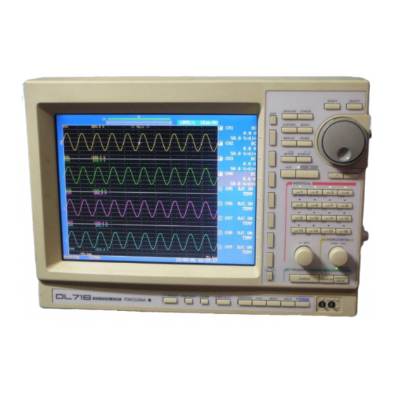
- Page 1 I-1102 Digital Scope IM 701830-01E 1st Edition...
- Page 2 Foreword Foreword Thank you for purchasing the YOKOGAWA DL716 Digital Scope. This User’s Manual contains useful information about the instrument’s functions and operating procedures as well as precautions that should be observed during use. To ensure proper use of the instrument, please read this manual thoroughly before operating it.
- Page 3 DL716 Main Body Check that the model name and suffix code given on the name plate of the rear panel match those on your order.
- Page 4 Checking the Contents of the Package Standard Accessories The following standard accessories are supplied with the instrument. Make sure that all items are present and undamaged. Power cord (one of the following power cords is supplied according to the instrument's suffix codes) Soft case UL/CSA standard VDE standard...
- Page 5 Checking the Contents of the Package Optional Accessories The following optional accessories are available. On receiving these optional accessories, make sure that all the items that you ordered have been supplied and that they are undamaged. If you have any questions regarding optional accessories, or if you wish to place an order, contact the dealer from whom you purchased the instrument.
-
Page 6: Safety Precautions
If this instrument is used in a manner not specified in this manual, the protection provided by this instrument may be impaired. Also, YOKOGAWA Electric Corporation assumes no liability for the customer's failure to comply with these requirements. - Page 7 To prevent an electric shock or fire, be sure to use the power cord supplied by YOKOGAWA. The main power plug must be plugged in an outlet with protective earth terminal. Do not invalidate protection by using an extension cord without protective earth.
- Page 8 How to Use this Manual Structure of the Manual This User’s Manual consists of 15 chapters, an Appendix and an Index as described below. Chapter Title Content Functions Introduces the unit’s features, functions, and operating principles. Please read this information to familiarize yourself with the unit’s capabilities.
- Page 9 How to Use This Manual Conventions Used in this Manual Unit k ....Denotes “1000”. Example: 100 kS/s K ....Denotes “1024”. Example: 640 KB (storage capacity of a floppy disk) Used Characters Alphanumerics enclosed in double quotation marks usually refer to characters and set values that appear on the screen and panel.
-
Page 10: Table Of Contents
Contents Foreword ............................... 1 Checking the Contents of the Package ..................2 Safety Precautions ............................5 How to Use this Manual ..........................7 Chapter 1 Functions Block Diagram ..........................1-1 Setting the Vertical and Horizontal Axes ..................1-2 Setting a Trigger ..........................1-7 Setting the Acquisition and Display Conditions ................ - Page 11 Contents Setting the Vertical Position of a Waveform ................... 5-5 Selecting Input Coupling ........................5-6 Selecting Probe Attenuation ......................5-7 Setting the Bandwidth ........................5-8 Zooming in Vertical Direction ....................... 5-10 Setting the Offset Voltage ......................5-11 5.10 Using the Linear Scaling Function ....................5-12 5.11 Inverting a Waveform ........................
- Page 12 Contents Setting the Waveform Labels ......................8-9 X-Y Waveform Display ......................... 8-10 Zooming the Waveform ......................... 8-12 8.10 Scrolling the Waveform (Replay) ....................8-15 Chapter 9 Waveform Analysis Measuring Waveforms using Cursors ....................9-1 Automatic Measurement of Waveform Parameters ................ 9-4 Setting Computing Range and Display Units, and Recomputing ...........
- Page 13 Contents 13.3 Setting the Screen Saver Function ....................13-4 13.4 Setting the Action on Trigger ......................13-5 13.5 Locking the Keys ..........................13-7 13.6 ON/OFF the Backlight ........................13-8 Chapter 14 Troubleshooting, Maintenance and Inspection 14.1 Breakdown Troubleshooting ......................14-1 14.2 Error Messages and Corrective Actions ..................
-
Page 14: Chapter 1 Functions
1.1 Block Diagram System Configuration HP-GL compatible plotter Centronics compatible Screen data printer External SCSI device Centronics Built-in printer interface Yokogawa's AG Series GP-IB/RS-232 SCSI Interface Waveform data interface Waveform data External clock input DL716 Video output Trigger out External trigger input... -
Page 15: Setting The Vertical And Horizontal Axes
1.2 Setting the Vertical and Horizontal Axes Time Axis ≡ Page 5-2. ≡ Setting the time axis When using the internal clock, set the time axis scale as a time duration per division of the grid. The setting range is 500 ns/div to 100 ks/div*. The time range in which waveform is displayed is “time axis setting x 10”, as the display range along the horizontal axis is 10 divisions. - Page 16 1.2 Setting the Vertical and Horizontal Axes Sample rate Changing the time axis causes a corresponding change in the sampling rate. Maximum sampling rate is 10MS. The waveform can only be displayed correctly at frequencies up to half the sample rate, due to Nyquist’s theorem*.
- Page 17 1.2 Setting the Vertical and Horizontal Axes Vertical Position (for Voltage/Logic Input Modules Only) ≡ Page 5-5. ≡ Since a total of eight input waveforms can be displayed, they may overlap each other, making observation difficult. In this case, the waveforms can be moved in the vertical direction so that can be observed more easily.
- Page 18 1.2 Setting the Vertical and Horizontal Axes Bandwidth Limit (For Voltage, Temperature, and Strain Modules) ≡ Page 5-8. ≡ The bandwidth limit of each module can be set individually. By setting a bandwidth limit, the noise component of the input signal can be deleted during waveform observation. Zooming in the Vertical Direction ≡...
- Page 19 1.2 Setting the Vertical and Horizontal Axes Temperature Measurement ≡ Page 5-16. ≡ Types of thermocouples The types of thermocouples available are as follows. K, E, J, T, L, U, N, R, S, B, W and A (KPvsAu7Fe) Temperature unit Can specify °C, °F or K.
-
Page 20: Setting A Trigger
1.3 Setting a Trigger Trigger Type ≡ Chapter 6. ≡ There are two principal trigger types which you can use with the instrument. Simple trigger Enhanced trigger Simple trigger → Pages 6-1 to 6-9. Triggers on the edge of a single signal (edge trigger). Enhanced trigger →... - Page 21 1.3 Setting a Trigger A Delay B trigger (Enhanced Trigger) → Page 6-12. A trigger is activated the 1st time condition B becomes true after condition A has become true and a preset time has elapsed. When pattern A : CH1 = L, CH2 = L, Enter, When pattern B : CH1 = H, CH2 =H, Enter, Delay = 2µs Trigger 2µs Pattern A is true Pattern B is true...
- Page 22 1.3 Setting a Trigger B>Time, B<Time, B Time out (Enhanced Trigger) → Page 6-17. A trigger is activated on the falling or rising edge of the pulse when the pulse width exceeds (or drops below) the preset time. In the case of a “Time out” trigger, a trigger is activated when the preset time elapses.
- Page 23 1.3 Setting a Trigger Trigger Mode ≡ Page 6-1. ≡ Conditions for updating displayed waveforms are set. The following two types of trigger mode are available. Auto-mode Displayed waveforms are updated each time a trigger is activated within a specified time (approximately 50 ms, referred to as the time-out period) and are updated automatically after each time-out period.
- Page 24 1.3 Setting a Trigger Trigger Hold-off ≡ Page 6-5. ≡ The trigger hold-off function temporarily stops detection of the next trigger once a trigger has been activated. For example, when observing a pulse train signal, such as a PCM code, display of the waveform can be synchronized with repetitive cycles;...
-
Page 25: Setting The Acquisition And Display Conditions
1.4 Setting the Acquisition and Display Conditions Record Length ≡ Page 7-1. ≡ Normally, the term record length refers to the number of data points acquired in the acquisition memory per channel. Display record length refers to the number of these data points that are actually displayed on the screen. - Page 26 1.4 Setting the Acquisition and Display Conditions Envelope mode In normal mode and averaging mode, the sample rate (the number of times data is acquired per second in the acquisition memory) drops if T/div is increased (refer to Appendix 1 “Relationship between the time axis setting, sample rate and record length”).
- Page 27 1.4 Setting the Acquisition and Display Conditions History Memory ≡ Page 7-6. ≡ The instrument automatically retains the last N waveforms recorded. The N value is equal to the maximum sequential-store acquisition count. The instrument retains all waveforms for the first N triggers;...
- Page 28 1.4 Setting the Acquisition and Display Conditions Display settings ≡ Chapter 8. ≡ Display format → page 8-1. • In order to make the observation of waveforms of multiple channels easy, you can split the screen to display the waveforms. The different ways to split the screen are as follows: Single (no split screen), Dual (2 screens) , Triad (3 screens) , Quad (4 screens), Hexa (6 screens), Octal (8 screens).
- Page 29 1.4 Setting the Acquisition and Display Conditions Display Interpolation ≡ Page 8-2. ≡ This feature selects the type of interpolation applied in areas where there are less than 500 sample points per 10 time-axis divisions. (These areas are referred to as interpolation areas.) Three settings are available.
- Page 30 1.4 Setting the Acquisition and Display Conditions X-Y Waveform Display ≡ Page 8-10. ≡ This feature plots the voltage values of one input waveform (on the X axis) against the voltage values of the others (on the Y axis, which have their display turned ON). The X-Y plot lets you view the relationship between the signal voltages.
- Page 31 1.4 Setting the Acquisition and Display Conditions Moving the display position of the waveform data ≡ Page 8-12 or 8-15. ≡ When the display record length is shorter than the set record length, some of the waveforms are not displayed on the screen. To display the waveforms that are not displayed on the screen, move the display position horizontally with “Main Position”...
-
Page 32: Analyzing The Waveform
1.5 Analyzing the Waveform Linear Scaling ≡ Page 5-12. ≡ It is possible to append a scaling constant A, an offset value B and a unit to the measurement value X of cursor or automated measurements. Linear scaling is useful, when applying a voltage divider ratio to the measurement values. - Page 33 1.5 Analyzing the Waveform Automated Measurements ≡ Page 9-4. ≡ Automatic measurement of waveform parameters This feature automatically measures selected waveform parameters, such as rise time and pulse width. You can select parameters separately for each channel, although you are limited to a total of 16 parameters for the entire system.
- Page 34 1.5 Analyzing the Waveform Power Spectrum Display ≡ Page 9-17. ≡ FFT (Fast Fourier Transform) computation can be performed on the input signal to display its power spectrum. This is useful when you want to check the frequency distribution of the input signal.
- Page 35 1.5 Analyzing the Waveform User Defined Computation ≡ Page 9-19. ≡ You can define a computing equation by combining the following operators. ABS(absolute value), SQR(square root), LOG(logarithm), EXP(exponent), BIN(binary computation), PWHH(pulse width), PWHL(pulse width), PWLH(pulse width), PWLL(pulse width), PWXX(pulse width), ATAN(arctangent), MEAN(moving average), DIF(differentiation), DDIF(2nd order differentiation), INTG(integral), IINTG(double integral), PH(phase), HLBT(Hilbert), P2(square), P3(cube), FILT1(digital filter), FILT2(digital filter), LS-(linear spectrum), RS-(rms value spectrum), PS-(power spectrum), PSD-(power spectrum...
-
Page 36: Other Useful Functions
1.6 Other Useful Functions Initialization ≡ Page 4-3. ≡ This function resets the key settings to the factory settings (default settings), and is useful when complex settings have been made and you want to cancel all of them at once. Auto Set-up ≡... - Page 37 You can save data in any of the following formats: HP-GL command format, Postscript, TIFF, and BMP. This means that you can easily insert the saved images into documents produced by conventional DTP software packages. Personal computer DL716 internal HDD External SCSI device Action on trigger ≡ Page 13-5. ≡...
-
Page 38: Chapter 2 Name And Use Of Each Part
Chapter 2 Name and Use of Each Part 2.1 Front Panel/Rear Panel • Front panel ESC key Menu keys (Page 2-4) Closes pop-up menu or soft key menu. Press a key to display the corresponding menu. Jog shuttle Changes the selected value or moves the cursor. The outer shuttles ring (outer ring) for fast setting increment. - Page 39 2.1 Front Panel/Rear Panel • Top View Built-in printer (Page 10-1) Handle Use the handle to lift and carry the unit. IM 701830-01E...
-
Page 40: Operation Keys/Jog Shuttle/Knobs
2.2 Operation Keys/Jog Shuttle/Knobs VERTICAL Group VERTICAL Keys CH1 to CH16 keys (Pages 5-1 to 5-17) 7 LOG/C1 8 LOG/C2 Displays the menu for setting the ON/OFF state, offset voltage, coupling, probe attenuation, preset, bandwidth limit, invert, linear scaling value for each channel. Also, it allows you to select the channel to operate with the V/div knob (for voltage modules only). - Page 41 2.2 Operation Keys/Jog Shuttle/Knobs Other Menus RESET SELECT MEASURE CURSOR HISTORY MATH REPLAY ZOOM ALL CH SETUP DISPLAY PROTECT SNAP SHOT CLEAR COPY MENU KEYBOARD FILE MISC HELP SHIFT STAET/STOP MEASURE key (Pages 9-4 to 9-8) Displays the menu for performing automatic measurement of waveform parameters. CURSOR key (Page 9-1) Displays the menu for cursor measurement.
- Page 42 2.2 Operation Keys/Jog Shuttle/Knobs CLEAR key (Page 4-7) Deletes the currently displayed waveform. COPY key (Chapter 10) Used for printing out hard copy of the screen data. If you press SHIFT + COPY , the screen displays a menu that you can use to print or save the screen image.
-
Page 43: Screens
2.3 Screens 1 V/div Displays the voltage axis sensitivity of the selected channel. 2 Acquisition mode Displayed when the acquisition mode is averaging, envelope, or box average. 3 Screen position bar Normal waveform Zooming waveform Zoom position Record length Record length Trigger position 500k 500k... -
Page 44: Chapter 3 Before Starting Observation And Measurement Of Waveforms
If you notice smoke or unusual odors coming from the instrument, immediately turn OFF the power and unplug the power cord. If such an irregularity occurs, contact your dealer or the nearest YOKOGAWA representative, as listed on the back cover of this manual. Power cord Nothing should be placed on the power cord;... -
Page 45: Installing
3.2 Installing Installation Conditions The instrument must be installed in a place where the following conditions are met. Flat horizontal location Set the instrument in the proper direction and in a level and stable place. If placed in an uneven or unstable place, printing quality decreases. - Page 46 3.2 Installing Installation Position Place the instrument in a horizontal position or with the rear panel facing down as shown in the figure below. When using the stand, pull it until it locks. When not in use, push the stand inwards to its original position.
-
Page 47: Connecting The Power Cord
3.3 Connecting the Power Cord Before Connecting the Power Make sure that you observe the following points before connecting the power. Failure to do so may cause electric shock or damage to the instrument. WARNING • Connect the power cord after confirming that the voltage of the power supply complies to the rated electric power voltage for the instrument. - Page 48 For details, refer to Section 4.2 “Initializing Settings” (page 4-3). If there is still no power even after the above points have been checked, contact your nearest YOKOGAWA representative as listed on the back cover of this manual.
-
Page 49: Setting The Date And Time
3.4 Setting the Date and Time Function Date (YY/MM/DD) The last two digits of the year are used to set the year (YY). Years 2000 to 2079 are represented by 00 to 79, and years 1980 to 1999 are represented by 80 to 99. -
Page 50: Installing The Input Module
3.5 Installing the Input Module WARNING • To prevent electric shock and damage to the instrument, make sure to turn OFF the power before installing or removing the input module. • Check that the input cable is not connected to the input terminals before installing or removing the input module. - Page 51 3.5 Installing the Input Module Installation procedure 1. Make sure the POWER switch is OFF. 2. Check the channel number indicated above the slots for installing the input modules on the right side of the instrument. Then, install the module along the guide. Holding the handles on the top and bottom of the input module, press hard until it clicks in place.
-
Page 52: Connecting A Probe
3.6 Connecting a Probe (For High-Speed Isolation/High-Speed Modules) Connecting a probe Connect the probe (or other input cables such as the BNC cable) to any of the input terminals of the High-Speed Isolation/High-Speed Module. WARNING • When connecting the item to be measured, make sure to turn OFF the power on the item. - Page 53 3.6 Connecting a Probe Points to Note when Connecting a Probe • When connecting a probe to the instrument for the first time, perform phase correction of the probe as described in Section 3.10 “Compensating the Probe (Phase Correction)” . Failure to do so may result in unstable gain across different frequencies, thereby preventing correct measurement.
-
Page 54: Connecting A Input Cable
3.7 Connecting a Input Cable (For High-Resolution, High Voltage, Isolation/High-Resolution, Isolation Modules) Connecting a measurement cable Connect the measurement cable to any of the input terminals of the High-Resolution, High- Voltage, Isolation/High-Resolution, Isolation Module. WARNING • When connecting the item to be measured, make sure to turn OFF the power on the item. -
Page 55: Connecting A Thermocouple
3.8 Connecting a Thermocouple (For Temperature Module) Connecting a thermocouple Connect the thermocouple strand directly to the input terminals of the temperature module. CAUTION • The temperature module is insulated from the main instrument. However, if a voltage exceeding the value indicated below is applied, it may cause damage to the input section. -
Page 56: Connecting A Logic Probe
• Each input terminal of the isolation logic probe is isolated from all other input terminals and the isolation logic probe is isolated from the DL716. • Make sure to turn off the instrument before connecting or disconnecting the 26-pin connector from the logic input connector. - Page 57 3.9 Connecting a Logic Probe Connecting the Logic Probe High-speed logic probe (700986) 1. Attach the accessory connecting lead (IC clip or alligator clip) to the logic probe, and lock the connector by clamping the lever inwards. To release the connecting lead from the logic probe, pull both levers outwards.
-
Page 58: Compensating The Probe (Phase Correction)
3.10 Compensating the Probe (Phase Correction) When making measurements using the probe on the High-Speed Isolation Module or High- Speed Module, make sure to phase correct the probe, first. CAUTION Never apply an external voltage to the COMP terminal, as damage to the instrument may result. -
Page 59: Connecting The Bridge Head
(For Strain Module) Connect a strain gauge bridge (bridge head) or strain gauge transducer and measure the strain. This section describes the procedures for connecting YOKOGAWA's bridge head (700932/ 700933) and precautions regarding the connection. For details on connecting other strain gauge bridges and strain gauge transducers, see the corresponding manuals. - Page 60 When using a bridge head with MIL Standard connector wiring The connector for the strain module is a NDIS connector*. Convert MIL to NDIS using YOKOGAWA's connector conversion cable 700935, then connect to the strain module. * A connector recommended by JSNDI (The Japanese Society for Non-destructive Inspection).
-
Page 61: Chapter 4 Common Operations
Chapter 4 Common Operations 4.1 Entering Values and Character Strings Entering a Value Direct entry using the special knob The following knobs can be used to enter values directly irrespective of the currently displayed menu. V/DIV and TIME/DIV knobs VERTICAL 7 LOG/C1 8 LOG/C2 µ... - Page 62 4.1 Entering Values and Character Strings Entering a Character String Date/time, file name and comment can be entered using the keyboard displayed on the screen. Operate the keyboard using the jog shuttle, SELECT key and arrow key to enter a character string as follows.
-
Page 63: Initializing Settings
4.2 Initializing Settings Function The initialization function allows you to reset parameter values which have been set using panel keys to the default (factory settings). This is very convenient when you have to cancel the previous settings or when you have to restart measurement from the beginning. Initialization Initialization means resetting parameters to their factory setting values. -
Page 64: The Auto Set-Up Function
4.3 The Auto Set-up Function Function The auto set-up function automatically sets each key setting, such as the V/div, T/div and trigger level, to the optimum value for the input signal. Center position after auto set-up : Sets the center position to “0 V”. Convenient when you want to see the relation between the ground level and the waveform. - Page 65 4.3 The Auto Set-up Function Settings made by auto set-up Waveform acquisition and display Acquisition mode Normal Acquisition count Infinite Record length 1 kword Accumulation mode Zoomed waveforms Traces set ON for display (realtime OFF) Vertical-axis settings V/div Set so that amplitude is between 2 divp-p and 7 divp-p (approximately) Offset voltage At Center 0 V...
-
Page 66: Starting And Stopping Acquisition
4.4 Starting and Stopping Acquisition Function The following three methods are available for starting and stopping acquisition. Using the START/STOP key : The data are continuously acquired and displayed according to the trigger mode setting (see section 6.1). Using the “Single Start” soft key : Pressing the soft key sets the trigger mode to normal (ACQ menu) mode. - Page 67 4.4 Starting and Stopping Acquisition Operating Procedure Using the START/STOP key Acquisition starts and stops alternately each time the START/STOP key is pressed. If the indicator on the START/STOP key is lit, acquisition is in progress. Using the “Single Start,” “Log Start” soft keys 1.
-
Page 68: The Snapshot And Clear Trace Functions
4.5 The Snapshot and Clear Trace Functions ≡ For a description of this function, refer to page 1-22. ≡ Function Snapshot This function retains the waveforms currently displayed on the screen. It also enables update of the display without stopping acquisition. Hence it is very useful when you want to compare waveforms. -
Page 69: Calibration
4.6 Calibration (For High-Speed Isolation/High-Speed/High-Resolution, High-Voltage, Isolation/High- Resolution, Isolation Modules) Function Calibration The following parameters can be calibrated. Perform calibration when highly accurate measurements are required. Ground level offset A/D converter gain Points for attention • Always allow the instrument to warm up for at least 30 minutes after the power is turned ON before starting calibration. -
Page 70: Using The Help Function
4.7 Using the Help Function Function Displaying a help window Pressing the HELP key displays the soft key menu which was in effect before the HELP key was pressed, or displays a help window which contains information related to jog shuttle menu settings. -
Page 71: Selecting The Time Base
4.8 Selecting the Time Base Function Selecting the time base Select the time base from the following choices. : Internal clock signal (TIME/DIV knob is effective) Ext : Clock signal input through the external clock input terminal (TIME/DIV knob is ineffective) When selecting “EXT”... - Page 72 4.8 Selecting the Time Base Precautions when sampling with an external clock signal • Clock signal must be set to continuous signal. You cannot use a burst signal. • You cannot set the acquisition mode to envelope mode or box average. •...
-
Page 73: Chapter 5 Vertical And Horizontal Axes
Chapter 5 Vertical and Horizontal Axes 5.1 Turning Channels ON/OFF Function The channels CH1 to CH8 can be displayed simultaneously. For channels which have their display is turned ON, the LED above the key lights. However, channels which do not have input modules installed cannot be turned ON. Note •... -
Page 74: Setting T/Div
5.2 Setting T/div ≡ For a description of this function, refer to page 1-2. ≡ Function The T/div setting is made by setting the time per division on the screen grid. T/div setting range Different types of modules can be installed simultaneously in this instrument. The available T/ div range is as follows. - Page 75 5.2 Setting T/div Display example When sampling a 10 kHz input signal at 5 MS/s CH3 : High-resolution, High-voltage, Isolation module CH7 : High-speed module Operating Procedure Turn the TIME/DIV knob to set the desired T/div. IM 701830-01E...
-
Page 76: Setting V/Div
5.3 Setting V/div (For High-Speed Isolation/High-Speed/High-Resolution, High-Voltage, Isolation/High- Resolution, Isolation Modules) ≡ For a description of this function, refer to page 1-3. ≡ Function The V/div (voltage axis sensitivity) setting is used to adjust the amplitude of the displayed waveform so that the waveform can be observed easily. The V/div setting is made by setting the voltage value per division on the screen grid. -
Page 77: Setting The Vertical Position Of A Waveform
5.4 Setting the Vertical Position of a Waveform (For High-Speed Isolation/High-Speed/High-Resolution, High-Voltage, Isolation/High- Resolution, Isolation/Logic Input Modules) ≡ For a description of this function, refer to page 1-4. ≡ Function Range of movement The vertical position can be moved in the range between ± 4 div from the center position in the waveform display frame. -
Page 78: Selecting Input Coupling
5.5 Selecting Input Coupling (For High-Speed Isolation/High-Speed/High-Resolution, High-Voltage, Isolation/High- Resolution, Isolation Modules) ≡ For a description of this function, refer to page 1-4. ≡ Function Input coupling The following three types of input coupling are available. : Acquires and displays only the AC content of the input signal. : Acquires and displays both the DC and the AC content of the input signal. -
Page 79: Selecting Probe Attenuation
Selecting Probe Attenuation ≡ For a description of this function, refer to page 1-4. ≡ For High-Speed Isolation/High-Speed Module, set the attenuation according to the probe being used. For High-Resolution, High-Voltage, Isolation/High-Resolution, Isolation Module, set the attenuation to 1:1. Function Probe attenuation for each channel can be selected from the following. -
Page 80: Setting The Bandwidth
5.7 Setting the Bandwidth (For High-Speed Isolation/High-Speed/High-Resolution, High-Voltage, Isolation/High- Resolution, Isolation/Temperature/Strain Modules) ≡ For a description of this function, refer to page 1-5. ≡ Function Bandwidth The following frequency bandwidth limit can be set on each input module. Each channel is set individually. - Page 81 5.7 Setting the Bandwidth Operating Procedure 1. Press one of the keys CH1 to CH16 to select the desired channel. 2. Press the “Bandwidth” soft key to change the band width setting. High-Resolution Isolation Module 3. Repeat the above steps as necessary to set the value on other channels. Note You can set the bandwidth separately for each channel.
-
Page 82: Zooming In Vertical Direction
5.8 Zooming in Vertical Direction (For High-Speed Isolation/High-Speed/High-Resolution, High-Voltage, Isolation/High- Resolution, Isolation/Logic Input Modules) ≡ For a description of this function, refer to page 1-5. ≡ Function The displayed waveform can be enlarged/reduced in vertical direction. It is useful when you wish to change the vertical axis setting after displaying waveforms using Single Start/Log Start (refer to page 4-6). -
Page 83: Setting The Offset Voltage
5.9 Setting the Offset Voltage (For High-Speed Isolation/High-Speed/High-Resolution, High-Voltage, Isolation/High- Resolution, Isolation Modules) ≡ For a description of this function, refer to page 1-5. ≡ Function The offset voltage can be set regardless of the input coupling setting. Offset voltage setting range The setting range varies depending on the input module as shown below. -
Page 84: Using The Linear Scaling Function
5.10 Using the Linear Scaling Function (For High-Speed Isolation/High-Speed/High-Resolution, High-Voltage, Isolation/High- Resolution, Isolation Modules, For strain modules, see section 5.16.) ≡ For a description of this function, refer to page 1-19. ≡ Function This function lets you apply linear scaling to the measurement values. If you set this feature ON, the screen displays the scaled results rather than the original measurements. - Page 85 5.10 Using the Linear Scaling Function Enabling/Disabling rounding of the upper and lower limits of the waveform display 1. Press the MISC key. 2. Press the “Next” soft key to display the “Next2/2” menu. Then, press the “Others” soft key. 3.
-
Page 86: Inverting A Waveform
5.11 Inverting a Waveform (For High-Speed Isolation/High-Speed/High-Resolution, High-Voltage, Isolation/High- Resolution, Isolation Modules) ≡ For a description of this function, refer to page 1-5. ≡ Function Relevant channels The input signals to channels CH1 to CH16 can be inverted independently of one another. Inversion is performed about the vertical position. -
Page 87: Setting The On/Off Of Channels And The V/Div With The All Channel Setting Menu
5.12 Setting the ON/OFF of Channels and the V/div with the All Channel Setting Menu Function The ON/OFF of each channel and the V/div setting are explained in pages 5-1 and 5-4 respectively. This section explains the procedure in displaying information on all the channels simultaneously and setting the ON/OFF and V/div settings for the individual channels. -
Page 88: Setting The Temperature Measurement
With the RJC turned off, if a voltage corresponding to a certain maximum temperature is applied at the input and the measured temperature is off as compared with the maximum temperature, the instrument may be damaged. Please contact your nearest YOKOGAWA dealer listed on the back cover of this manual. 5-16... - Page 89 5.13 Setting the Temperature Measurement Operating Procedure 1. Press one of the keys (channel key which has the Temperature Module installed) CH1 to CH16 to select the channel. Select the type of thermocouple 2. Press the “Type” soft key to select the desired type. Set the display range 3.
-
Page 90: Setting The Logic Probe
5.14 Setting the Logic Probe (For Logic Input Module and /N1 32-bit extended logic input) Function ON/OFF of bit display:Bit Display Allows you to select whether or not to display the waveform for each bit. Mapping the logic waveform: Bit Mapping OFF : The spaces for the bit waveforms that are turned OFF are maintained. -
Page 91: Setting The Strain Measurement
5.15 Setting the Strain Measurement (For Strain Module) Function Selecting the measurement range : Range Select the range according to the magnitude of the strain to be measured. 20000uSTR, 10000uSTR, 5000uSTR, 2000uSTR, 1000uSTR uSTR stands for 10 strain. For the measurement range, see section 15.24. Selecting the display range : Upper Scale/Lower Scale To make the viewing of the measured waveform easier, you can change the upper and lower limits of the display range according to the input. - Page 92 5.15 Setting the Strain Measurement Executing balancing : Balance The unbalanced portion of the bridge resistance is automatically corrected. The balancing takes a few seconds. Balance range : ±10000uSTR Precautions when making strain measurements • If there is no strain gauge bridge (bridge head) or strain gauge transducer connected to the channel you wish to balance, calibration fails.
- Page 93 5.15 Setting the Strain Measurement Execute balancing 8. Press the “Balance” soft key to display the channel selection menu. 9. Turn the jog shuttle to move the cursor to the channel that you wish to balance. 10. Press the SELECT key to turn it ON. 11.
-
Page 94: Using The Linear Scaling Function For The Strain
5.16 Using the Linear Scaling Function for the Strain (For Strain Module) Function Linear Scaling Selecting the linear scaling method : Linear Scaling • Select the linear scaling method from the following. • OFF No linear scaling is performed. • Ax+B The setting range and the initial setting of the scaling coefficient A and offset value B are the same as described in section 5.10 “Using the Linear Scaling Function.”... - Page 95 5.16 Using the Linear Scaling Function for the Strain Operating Procedure 1. Press one of the keys (channel key that has the strain module installed), CH1 to CH16 , to select the channel. 2. Press the “Next1/2” soft key. Select the linear scaling 3.
- Page 96 5.16 Using the Linear Scaling Function for the Strain When “P1–P2” is selected 4. Press the “P1:X/P1:Y” soft key and set the jog shuttle action to “P1:X.” “P1:X” is displayed in the “Get Measure” soft key. 5. Press the “Get Measure” soft key to read in the measured value into P1:X or set the value with the jog shuttle.
-
Page 97: Displaying The Setup Menu Over The Entire Screen (Full Screen Setup)
5.17 Displaying the Setup Menu over the Entire Screen (Full Screen Setup) Function You can display the setup menu of all channels over the entire screen and set the parameters. The setting parameters are the same as those of the channel key. Operating Procedure 1. -
Page 98: Chapter 6 Triggering
Chapter 6 Triggering 6.1 Setting the Trigger Mode ≡ For a description of this function, refer to page 1-10. ≡ Function Auto mode Auto mode is the one which is used normally. The display is updated in the following two cases. -
Page 99: Selecting A Channel For Setting Trigger Hysteresis And Trigger Level
6.2 Selecting a Channel for Setting Trigger Hysteresis and Trigger Level Function Selects the channel (trigger source) for setting parameters such as trigger hysteresis and trigger level. If you use a simple trigger, only the selected channel serves as the trigger source. If you use an enhanced trigger, the trigger source is generated using all channels selected within the “Set Pattern”... -
Page 100: Setting Trigger Hysteresis For Channels 1 To 16
6.3 Setting Trigger Hysteresis for Channels 1 to 16 (For High-Speed Isolation/High-Speed/High-Resolution, High-Voltage, Isolation/High- Resolution, Isolation/Temperature/Strain Modules) ≡ For a description of this function, refer to page 1-10. ≡ Function Setting the trigger hysteresis Allow the trigger level to have a width, so that the trigger does not get activated due to small fluctuations in the signal. -
Page 101: Setting The Trigger Level
6.4 Setting the Trigger Level (For High-Speed Isolation/High-Speed/High-Resolution, High-Voltage, Isolation/High- Resolution, Isolation/Temperature/Strain Modules) ≡ For a description of this function, refer to page 1-10. ≡ Function Trigger level setting range CH1 to CH16 : 8 divisions For voltage modules, the setting resolution is 0.1 div. If the voltage scale is 2 mV/div, for example, the setting resolution will be 0.2 mV. -
Page 102: Setting The Hold Off Time
6.5 Setting the Hold off Time ≡ For a description of this function, refer to page 1-11. ≡ Function This function prevents a trigger from being activated for a specified time, even if the trigger conditions are met during this time. This is useful when you want to activate a trigger after a certain repetitive period of time as illustrated in the example below. -
Page 103: Setting The Trigger Position
6.6 Setting the Trigger Position ≡ For a description of this function, refer to page 1-11. ≡ Function Trigger Position Specify which part of the acquired waveform in the acquisition memory to display on the screen by setting the trigger position. If the trigger delay is 0 s, the trigger position is equivalent to the trigger point. - Page 104 6.6 Setting the Trigger Position Operating Procedure 1. Press the POSITION/DELAY key. 2. Press the “ Position” soft key. 3. Turn the jog shuttle to set the trigger position. You can change the setting a digit using the arrow keys (located below the jog shuttle). You can reset the position to 50% by pressing the RESET key.
-
Page 105: Setting The Trigger Delay
6.7 Setting the Trigger Delay ≡ For a description of this function, refer to page 1-11. ≡ Function Although the display usually shows the waveform before and after the trigger point, using the delay function, it is possible to display the acquired waveform after a fixed time period elapses. Setting range for trigger delay 0 to 1 s (Resolution is 500 ns) Trigger position... -
Page 106: Setting The Edge Trigger (Simple)
6.8 Setting the Edge Trigger (SIMPLE) ≡ For a description of this function, refer to page 1-7. ≡ Function An edge trigger is generated when the trigger source crosses the trigger level in the specified direction. Setting the trigger mode Refer to Section 6.1. -
Page 107: Setting The A→B (N) Trigger (Enhanced)
6.9 Setting the A→B (n) Trigger (ENHANCED) ≡ For a description of this function, refer to page 1-7. ≡ Function This function activates a trigger the n’th time condition B becomes true after condition A has become true. Condition A, B settings •... - Page 108 6.9 Setting the A→B (n) Trigger (ENHANCED) Setting the condition A 4. Press the “ Set Pattern” soft key to display the A →B(n) trigger setting menu. 5. Turn the jog shuttle to move the cursor to the <Parallel A> “Condition.” 6.
-
Page 109: Setting The A Delay B Trigger (Enhanced)
6.10 Setting the A Delay B Trigger (ENHANCED) ≡ For a description of this function, refer to page 1-8. ≡ Function This function activates a trigger the 1st time condition B becomes true after condition A has become true and the preset time has elapsed. Condition A, B settings •... - Page 110 6.10 Setting the A Delay B Trigger (ENHANCED) Setting the condition A 4. Press the “ Set Pattern” soft key to display the A Delay B trigger setting menu. 5. Turn the jog shuttle to move the cursor to the <Parallel A> “ Condition”. 6.
-
Page 111: Setting The Edge On A Trigger (Enhanced)
6.11 Setting the Edge on A Trigger (ENHANCED) ≡ For a description of this function, refer to page 1-8. ≡ Function This function activates a trigger when an OR trigger (an edge trigger) occurs while condition A is true. Condition A, B settings •... - Page 112 6.11 Setting the Edge on A Trigger (ENHANCED) Setting condition A to true/false 4. Press the “ Set Pattern” soft key to display the Edge on A trigger setting menu. 5. Turn the jog shuttle to move the cursor to the <Parallel A> “ Condition.” 6.
-
Page 113: Setting The Or Trigger (Enhanced)
6.12 Setting the OR Trigger (ENHANCED) ≡ For a description of this function, refer to page 1-8. ≡ Function This function activates a trigger when either of the selected edge triggers occurs. For example, a trigger can be caused on either the rising edge of CH1 or CH2. Edge OR Select from the following. -
Page 114: Setting The B>Time, B
6.13 Setting the B>Time, B<Time or B Time Out Trigger (ENHANCED) ≡ For a description of this function, refer to page 1-9. ≡ Function B>Time : Trigger occurs when condition B goes false after holding true for the preset pulse width. - Page 115 6.13 Setting the B>Time, B<Time or B Time Out Trigger (ENHANCED) Operating Procedure Setting the trigger type 1. Press the ENHANCED key. 2. Press the “ Type” soft key to display the trigger type menu. 3. Keep pressing the “ Type” soft key to select “ B>Time,” “ B<Time,” or “ B Time Out.” Setting the channel status for condition B 4.
-
Page 116: Setting The Window Trigger (Enhanced)
6.14 Setting the Window Trigger (ENHANCED) ≡ For a description of this function, refer to page 1-9. ≡ Function Waveform for window trigger Select the waveform to set the window trigger from the following. CH1 to CH16 (except for Logic Input Module) Trigger condition You can set trigger conditions on all channels. - Page 117 6.14 Setting the Window Trigger (ENHANCED) Operating Procedure Set the trigger type 1. Press the ENHANCED key. 2. Press the “ Type” soft key to open the Trigger Type menu. 3. Press the “ Type” soft key as necessary to select Window. Set the trigger condition 4.
-
Page 118: Setting The Timer Trigger
6.15 Setting the Timer Trigger Function The trigger is activated at specified time intervals from the specified time. The following time intervals are selectable. Trigger position As in the normal trigger, you can set the trigger position to observe the phenomenon occurring around the specified time. -
Page 119: Chapter 7 Acquisition And Display
Chapter 7 Acquisition and Display 7.1 Setting the Record Length ≡ For a description of this function, refer to page 1-12. ≡ Function The record length sets the amount of data to be written into the acquisition memory. Maximum length depends upon the machine model. Available length settings are as follows. 16M/CH models (/M3) : 1 k, 10 k, 40 k, 100 k, 200 k, 400 k, 1 M, 2 M, 4 M, 8 M, 16 M, 32 M... -
Page 120: Acquisition Mode
7.2 Acquisition Mode ≡ For a description of this function, refer to page 1-12. ≡ Function You can select any of five acquisition modes, as follows. The default selection is Normal. Normal The instrument writes sample data into acquisition memory without performing special processing. - Page 121 7.2 Acquisition Mode Important information about the averaging mode • Averaging mode is useful when working with repetitive waveforms. • Correct averaging is not possible if the waveform has imperfect triggering, since synchronization will be poor and the displayed waveform will be distorted. When working with this type of signal, set the trigger mode to Normal, so that the waveform display is updated only when the trigger occurs.
-
Page 122: Sequential Store Mode
7.3 Sequential Store Mode ≡ For a description of this function, refer to page 1-13. ≡ Function Acquisition count Available numerical settings are as follows. If you set the value to Infinite, acquisition will continue until you switch it off with the START/ STOP key. -
Page 123: Box Average Mode
7.4 Box Average Mode (For High-Speed Isolation/High-Speed Modules) ≡ For a description of this function, refer to page 1-13. ≡ Function Under normal conditions, the instrument constantly samples the input signal at 10 MS/s, extracts values according to the T/div setting from the sampled data, and writes to the acquisition memory. -
Page 124: Using The History Memory
7.5 Using the History Memory ≡ For a description of this function, refer to page 1-14. ≡ Function The acquisition memory retains waveform records generated by the most recent triggers. The number of stored records is equivalent to the maximum number of records that can be obtained when using sequential-store mode. - Page 125 7.5 Using the History Memory Precautions to be taken when recalling data from the history memory • Acquisition will stop when the history memory menu is displayed. It is not possible to recall waveform data from the history memory while acquisition in progress. •...
- Page 126 7.5 Using the History Memory Operating Procedure Recalling data from the history memory 1. Press the HISTORY key. 2. Press the “ Selected Record No.” soft key. The “ Selected Record No.” can now be set using the jog shuttle. 3.
-
Page 127: Realtime Print To The Built-In Printer
7.6 Realtime Print to the Built-in Printer ≡ For a description of this function, refer to page 1-14. ≡ Function The waveform (screen image data) is continuously printed to the built-in printer like a recorder. Waveform to realtime print All of the original waveforms displayed on the screen are realtime printed. If only the X-Y waveform/zoom waveform is displayed (the original waveform is not displayed), then realtime printing cannot be performed. - Page 128 7.6 Realtime Print to the Buil-in Printer Stopping the realtime print If the waveform acquisition is stopped by pressing the START/STOP key, the print out is also stopped even if it is within the set record time. Points to note when realtime printing •...
-
Page 129: Realtime Record To The Internal Hard Disk (Optional)
7.7 Realtime Record to the Internal Hard Disk (Optional) ≡ For a description of this function, refer to page 1-14. ≡ Function The data can be realtime recorded to the internal hard disk (option). The internal hard disk contains the following drives: Realtime: This drive is used for realtime recording. - Page 130 7.7 Realtime Record to the Internal Hard Disk (Optional) Restore the realtime recorded data The previous realtime recorded data can be recalled to the real time record area by pressing the “ Restore HD” soft key. Note Please note that the operation is different on the DL708/DL708E. Saving and loading the realtime recorded waveform data See section 11.6 “Saving/Loading Waveform Data.”...
- Page 131 7.7 Realtime Record to the Internal Hard Disk (Optional) Operating Procedure 1. Press the ACQ key. Selecting the realtime record destination 2. Press the “ Realtime Out” soft key to select “ HD.” Setting the record time (when executing with the START/STOP key) 3.
-
Page 132: Chapter 8 Display
Chapter 8 Display 8.1 Changing the Display Format Function Main Format Single: 1 waveform window Quad : 4 waveform windows Dual : 2 waveform windows Hexa : 6 waveform windows Triad : 3 waveform windows Octal : 8 waveform windows Mapping Auto : Windows are arranged from top to bottom in order: CH1, CH2,..., Math1, Math2. -
Page 133: Setting The Interpolation Method
8.2 Setting the Interpolation Method ≡ For a description of this function, refer to page 1-16. ≡ Function Interpolate Any area along the time axis having less than 500 points per 10 divisions is recognized as an interpolation area. If you leave interpolation off, these points will appear as discrete dots (so that the display will show gaps between dots or vertical lines). - Page 134 8.2 Setting the Interpolation Method Operating Procedure Set the interpolation method 1. Press the DISPLAY key. 2. Keep pressing the “Interpolate” soft key to select the necessary method. Set the compression method (Only if Interpolate=OFF.) 3. Keep pressing the “Display Style” soft key to select the necessary method. IM 701830-01E...
-
Page 135: Changing The Graticule
8.3 Changing the Graticule Function The graticule type can be selected from the following 3 types. Grid( ) Frame( ) Cross( ) Operating Procedure 1. Press the DISPLAY key. 2. Press the “Graticule” soft key to select one of the three graticule types. IM 701830-01E... -
Page 136: Accumulated Waveform Display
8.4 Accumulated Waveform Display ≡ For a description of this function, refer to page 1-16. ≡ Function Normally the display is updated each time a trigger is activated. Therefore, it is difficult to observe instantaneous disturbance of a waveform. To solve this problem, the accumulation function has been provided. - Page 137 8.4 Accumulated Waveform Display Operating Procedure Selecting averaging mode 1. Press the DISPLAY key. 2. Press the “Accumulate” soft key to select “OFF”, “Persist” or “Color.” Proceed to step 3 if you have selected “Persist”, or to step 4 if you have selected “Color”. Setting the accumulative count (when “Persist”...
-
Page 138: Turning The Extra Window On/Off
8.5 Turning the Extra Window ON/OFF ≡ For a description of this function, refer to page 1-15. ≡ Function An extra window is provided to display information other than waveforms when waveforms obscure the information in the display area. The following three types of information can be displayed in the extra window. -
Page 139: Turning Display Of The Scaling Value And Trigger Mark On/Off
8.6 Turning Display of the Scaling Value and Trigger Mark ON/OFF ≡ For a description of this function, refer to pages 1-15. ≡ Function For each channel, you can select to display scale values at the top and bottom of the vertical axis. -
Page 140: Setting The Waveform Labels
8.7 Setting the Waveform Labels ≡ For a description of this function, refer to page 1-15. ≡ Function Label display ON/OFF (Trace Label) Use this parameter to select whether or not to include waveform labels (channel identification labels) on the display. Entering customized labels You can use the Define Label feature to enter customized labels for each channel. -
Page 141: X-Y Waveform Display
8.8 X-Y Waveform Display ≡ For a description of this function, refer to page 1-17. ≡ Function Assignment of X (horizontal) and Y (vertical) axes X axis : Any trace (CH1, ..., CH16, Math1, ..., Math8) Y axis : All other traces for which display is set ON. Display format (Mode) You can choose either of the following display formats. - Page 142 8.8 X-Y Waveform Display Operating Procedure 1. Press the SHIFT+DISPLAY key (X-Y). Set the display format 2. Press the “MODE” soft key as necessary to select the format: “OFF”, “T-Y & X-Y”, or “X- Y”. 3. Press the “X Trace” soft key to set the jog shuttle action to “X Trace.” Then turn the jog shuttle to select the X-axis waveform (CH1, ..., Math8).
-
Page 143: Zooming The Waveform
8.9 Zooming the Waveform ≡ For a description of this function, refer to page 1-17. ≡ Function The instrument can display up to two zoom windows for each of waveforms selected for display. You can set the zoom function on or off for each of the display waveforms. Note that zooming cannot function on areas with less than 11 display points. - Page 144 8.9 Zooming the Waveform Moving the range in which to perform automatic measurement of waveform parameters: Fit Measure Range Pressing the “Fit Measure Range...” soft key moves the range in which to perform the automatic measurement of waveform parameters to the ends of the Z1 or Z2 waveform display frame. Whether it moves to the ends of the Z1 frame or the Z2 frame depends upon how the zoom waveform is being displayed.
- Page 145 8.9 Zooming the Waveform Page Scroll (when using Main mode only) 12. Press the “Page Scroll Direction” soft key to select “<<” or “>>.” 13. The waveform display position moves by one screen, every time the “Page Scroll” soft key is pressed. 8-14 IM 701830-01E...
-
Page 146: Scrolling The Waveform (Replay)
8.10 Scrolling the Waveform (Replay) Function Auto Scroll Automatically scrolls the waveform until the “Auto Scroll Start/Stop” key is pressed. Page Scroll This function is the same as the page scroll function in the ZOOM menu. The waveform scrolls one page at a time. Scroll Using the Jog Shuttle Turning the jog shuttle scrolls the waveform. -
Page 147: Chapter 9 Waveform Analysis
Chapter 9 Waveform Analysis 9.1 Measuring Waveforms using Cursors ≡ For a description of this function, refer to page 1-19. ≡ Function Restrictions Cursor measurements cannot be used with the following waveform types. • Snapshot waveforms • Accumulated waveforms (except for most recent waveform) Cursor types and measurement values •... - Page 148 9.1 Measuring Waveforms using Cursors Marker jump to the original waveform display frame: Marker Jump Sometimes the marker cursor goes out of the waveform display frame when the waveform is being zoomed or when the display record length is shorter than the set record length. In such case, this allows the marker cursor to jump to the center of the waveform display frame.
- Page 149 9.1 Measuring Waveforms using Cursors Setting the reference width (only when the cursor type is set to “UserDefine”) Moving Cursors Ref1 and Ref2 7. Press the “Ref1/Ref2” soft key and set the jog shuttle action to “Ref1.” 8. Move Ref1 with the jog shuttle, and set the zero point. 9.
-
Page 150: Automatic Measurement Of Waveform Parameters
9.2 Automatic Measurement of Waveform Parameters ≡ For a description of this function, refer to page 1-19. ≡ Function You use this function to generate automatic measurements of waveform characteristics based on data in the acquisition memory. Restrictions Automatic measurement cannot be used with the following waveform types. •... - Page 151 9.2 Automatic Measurement of Waveform Parameters Measurement Range (Time Range) As the default, measurement starts at -4div from the display center and extends to +4div, but you can shorten the range. You make the setting by positioning two vertical lines: a dot-dash line for the start point, and a dashed line for the end point.
- Page 152 9.2 Automatic Measurement of Waveform Parameters • Other parameters Histo : Frequency distribution of voltage values Int1TY : Area under positive amplitude Int2TY : (Area under positive amplitude) – (area under negative amplitude) Int1XY : Summation of triangular area in X-Y waveform Ing2XY: Summation of trapezoidal area in X-Y waveform * For details about area calculations, refer to Appendix 3 (page App-4).
- Page 153 9.2 Automatic Measurement of Waveform Parameters Setting the measurement range 9. Press the “Time Range” soft key. 10. Turn the jog shuttle to set the desired measurement range. Setting the delay start point (for measurement of RDelay and FDelay) 11. Keep pressing the “Delay Ref” soft key to select the desired source of the delay start point from “Trig”...
- Page 154 9.2 Automatic Measurement of Waveform Parameters Setting the distal and proximate points (Unit) 12. Press the “Next” soft key to display the “Next 2/2” menu. 13. Press the “Dist/Prox Mode” soft key as necessary to select Unit. 14. Press the “Trace” soft key to select the trace target. 15.
-
Page 155: Setting Computing Range And Display Units, And Recomputing
9.3 Setting Computing Range and Display Units, and Recomputing Function Computing range (Start Point/End Point) • The instrument can execute automatic computation on up to 400 kW. When displaying a waveform of 400 kW or more, computation on all of the data cannot be performed at once. •... -
Page 156: Waveform Addition, Subtraction And Multiplication
9.4 Waveform Addition, Subtraction and Multiplication Function Use the following procedure to add, subtract, or multiply waveforms from two different channels. Channel allocation is as follows. Math1 : (Basic) CH1 and CH2; or CH1 and CH5 Math2 : (Basic) CH1 and CH3; or CH3 and CH7 Math1 and Math2 calculations can operate simultaneously. -
Page 157: Binary Computation
9.5 Binary Computation Function Use this function to convert the CH1, CH2, or Math1 waveform to a two-level digital signal (0 and 1 levels only). Conversion is made with respect to two specified threshold levels, as illustrated below. Upper Lower Note Binary computation is operative on every channel. - Page 158 9.5 Binary Computation Setting the threshold 6. Press the “Next” soft key to display the “Next 2/2” menu. 7. Press the “Threshold Trace” soft key to select the channel for which the threshold is to be set. 8. Press the “Threshold Up” soft key. The upper threshold level can now be set using the jog shuttle.
-
Page 159: Phase Shifted Addition, Subtraction And Multiplication
9.6 Phase Shifted Addition, Subtraction and Multiplication Function This function lets you shift the waveform from one channel (phase shift) and then add, subtract, or multiply the shifted waveform against the waveform on another channel. Channel allocations are as follows. Math1 (Phase) CH1 and CH2;... - Page 160 9.6 Phase Shifted Addition, Subtraction and Multiplication Setting the addition and subtraction type 4. Press the “Math1” or “Math2” soft key to display the Math1 menu. 5. Press the same soft key again to select the desired type. Setting the phase shift 6.
-
Page 161: Simultaneous Binary Computation And D/A Conversion Of All Channels
9.7 Simultaneous Binary Computation and D/A Conversion of All Channels Function Simultaneous binary computation on all channels Binary computation can be performed on all channels simultaneously. Binary computation cannot be performed on inputs from the following types of channels. The computed waveforms of these channels are not displayed. - Page 162 9.7 Simultaneous Binary Computation and D/A Conversion of All Channels Operating Procedure Selecting the computation mode 1. Press the MATH key. 2. Press the “Mode” soft key to display the math menu. 3. Keep pressing the “Mode” soft key until “Binary” is selected. Setting the simultaneous binary computation type 4.
-
Page 163: Displaying Power Spectrums
9.8 Displaying Power Spectrums ≡ For a description of this function, refer to page 1-21. ≡ Function This function displays the power spectrum of the waveform on CH1/2/5. Math1(Basic) : PS(C1), PS(C2) Math2(Basic) : PS(C5) If CH1/2/5 is set to logic input, however, the power spectrum is not displayed. Points Select 1000, 2000, or 10000. -
Page 164: Manual Scaling
9.9 Manual Scaling ≡ For a description of this function, refer to page 1-20. ≡ Function Normally, the computed waveform is displayed using auto scaling according to the results of the computation. Using manual scaling, you can set the upper and lower limit values of the computed waveform display to any desired value. -
Page 165: Executing User Defined Computation (Optional)
9.10 Executing User Defined Computation (Optional) =For a description of this function, refer to page 1-22.= Function The following operators can be combined to make computations. Available operators Operator Example Description +,-,X,/ C1+C2 Display the arithmetic operation of the specified waveform ABS(M1) Display the absolute value of the specified waveform SQR(C2) - Page 166 • Only two operators can be used in an equation for FILT1 and FILT2. Setting Range (Start Point/End Point) The DL716 can perform computation on up to 100 kW of data. However, when there are only two or less equations, the computation can be performed on up to 400 kW of data.
- Page 167 9.10 Executing User Defined Computation (Optional) The allowable range for the threshold level varies depending on the specified waveform as shown below. Channel waveform: 8 div within the display screen (setting resolution is 0.1 div) Math waveform: –1.0000E+30 to 1.0000E+30 For a description of the FFT, refer to points, FFT frequency band, and window in Section 9.8 “Displaying Power Spectrums.”...
- Page 168 9.10 Executing User Defined Computation (Optional) Setting the threshold level If “BIN” or pulse width computation is specified in the computing equation, set the threshold level with the jog shuttle. 7. Press the “Next” soft key to display the “Next 2/3” menu. 8.
- Page 169 9.10 Executing User Defined Computation (Optional) Setting the number of points for the FFT and the time window If “FFT” is specified in the computing equation, set the following settings. 7. Press the “Next” soft key to display the “Next 3/3” menu. 8.
-
Page 170: Chapter 10 Output Of Screen Data
10.1 Loading Paper Roll in Printer Printer Roll Chart Use only YOKOGAWA’s roll charts. When you are using the printer for the first time, use the roll chart supplied with the instrument. When your roll charts have run out, purchase more from your dealer or YOKOGAWA sales offices listed on the back cover of this manual. - Page 171 10.1 Loading Paper Roll in Printer Operating Procedure While pressing the lock release lever towards “OPEN” lift the handle on the left of the printer cover Lock release lever and open the cover. Handle Printer cover Move the release arm, located on the right near the front, to the “MAN FEED”...
-
Page 172: Feeding The Chart
10.2 Feeding the Chart Function The roll chart can be fed to check whether the chart has been loaded properly or to skip dirty sections. Points for attention The roll chart cannot be fed during acquisition. Operating Procedure 1. Press the SHIFT key. Functions marked in purple on the panel are now operative. -
Page 173: Outputting To Printer
10.3 Outputting to Printer Function Output type Following three output types are available for printing to the built-in printer. • Normal : The display screen is printed in normal size. Split Mode settings cannot be made. • Long : Enlarge the waveform displayed on the screen by a factor of 2 to 50 taking 10 div on the time axis to be one page and print (long copy) The following magnifying factors are available. - Page 174 10.3 Outputting to Printer Selecting the output type 5. Press the “type” soft key to display the output format menu. 6. Keep pressing the “type” soft key to select the desired output type from “Normal” to “Long*50” or “All.” Split print ON/OFF 7.
-
Page 175: Outputting To A Printer With A Centronics Interface
10.4 Outputting to a Printer with a Centronics Interface Function This instrument allows screen image data to be printed to an external printer using the Centronics interface. CAUTION • Use the Centronics printer connection cable (B9946YY) to connect the external printer and the instrument. - Page 176 10.4 Outputting to a Printer with a Centronics Interface Points for attention • No data can be output to the printer during acquisition. • When both pre-zoom waveform and zoomed waveform are displayed, only the pre-zoom waveform is applicable to long copy. •...
-
Page 177: Gp-Ib/Rs-232 Interface : Data Output And Format Selection
10.5 GP-IB/RS-232 Interface : Data Output and Format Selection Function Output data format Screen data can be output in the following formats to external equipment, such as a personal computer, via the GP-IB interface or the RS-232 interface. When the output data format is set to HP-GL, the maximum number of waveforms that can be output is 52. - Page 178 10.5 GP-IB/RS-232 Interface : Data Output and Format Selection SP0 (Append SP0) SP0 is an HP-GL command for setting the plotter’s pen. However, with some plotters, this command is sometimes assigned to another function. The SP0 command is sent at the end of data transmission if “Yes”...
- Page 179 10.5 GP-IB/RS-232 Interface : Data Output and Format Selection Connection Procedure Connecting the plotter 1. Turn OFF the power to both the instrument and the plotter. 2. Connect the plotter to the instrument using the GP-IB cable or the RS-232 cable. 3.
- Page 180 10.5 GP-IB/RS-232 Interface : Data Output and Format Selection Setting the paper size, plotting size, pen speed and pen assignment (for only HP- GL format) 7. Press the “Plotter Setup” soft key to display the plotter setting menu. 8. Turn the jog shuttle to move the cursor to “Paper Size.” 9.
-
Page 181: Outputting To Floppy Disk, Internal Hard Disk (Optional) Or External Scsi Device
10.6 Outputting to Floppy Disk, Internal Hard Disk (Optional) or External SCSI Device Function Output data format The data can be saved to the specified media in the following formats. The extension identifiers, which are attached automatically, and the file size (when half-tone is OFF) are shown below for your reference. - Page 182 10.6 Outputting to Floppy Disk, Internal Hard Disk (Optional) or External SCSI Device Selecting the output format and setting the half tone (except for HP-GL format) 5. Press the “Format” soft key to display the output format menu. 6. Keep pressing the “Format” soft key to select the desired output format: “HP-GL” to “BMP.”...
-
Page 183: Chapter 11 Saving/Loading The Data/Connecting To The Pc
Chapter 11 Saving/Loading the Data/Connecting to the PC 11.1 Floppy Disks Types of floppy Disk which can be used The following types of 3.5-inch floppy disks can be used. Floppy disks can also be formatted using this instrument. 2HD type : MS-DOS format, 1.2 MB or 1.44 MB 2DD type : MS-DOS format, 640 KB or 720 KB Inserting a Floppy Disk into the Drive Hold the floppy disk with the label facing up and the shuttered-side facing towards the drive,... -
Page 184: Internal Hard Disk (Optional)
11.2 Internal Hard Disk (Optional) CAUTION When using the instrument in an environment having vibration, turn OFF the power of the internal hard disk. Function The power of the internal hard disk can be turned ON/OFF on this instrument. The internal hard disk can be protected from the vibration by turning the power OFF. -
Page 185: Connecting A Scsi Device
Support for SCSI devices The instrument supports most but not all SCSI devices. If you need to know whether you can use a particular SCSI model, please consult your dealer or any of the Yokogawa affiliates listed at the back of this manual. -
Page 186: Formatting Disks
• Do not remove the disk or turn OFF the power while formatting is in progress (“Format...”). The media may be damaged. • If the DL716 cannot access the formatted media, reformat the media on the DL716. Since all data will be lost when you format the media, back up the data beforehand. - Page 187 11.4 Formatting Disks Precautions to be taken during formatting • If a floppy disk that contains data is formatted, all the data on the disk will be lost. • When a floppy disk is inserted into the drive, the “Access..” message will flash, indicating that processing is in progress.
- Page 188 11.4 Formatting Disks Selecting the formatting mode (only for external SCSI device) 6. Press the “Mode” soft key to select “Normal” or “Quick.” Selecting the format type (only for floppy disks) 6. Keep pressing the “Type” soft key until the desired format type is selected from “2DD 640K”...
-
Page 189: Selecting The Medium And Directory
11.5 Selecting the Medium and Directory Function Selecting the media You can save waveform and setting data to three storage locations: Floppy disk (FD) Internal hard disk (HD) External SCSI device (SCSI) * Internal hard disk and SCSI interface are options. * When selecting the external SCSI device, have the “External ID”... -
Page 190: Saving/Loading Waveform Data
11.6 Saving/Loading Waveform Data CAUTION • Never remove the disk or turn OFF the power while the drive is processing the insertion of the disk or while saving (“Access...”). The media may be damaged. Function Savable data • The currently displayed waveform on CH1 to CH16, Math1 to Math8. However, accumulated waveforms cannot be saved.) •... - Page 191 11.6 Saving/Loading Waveform Data Precautions to be taken when storing waveform data • Storing is not possible while acquisition is in progress. To enable storing, press the START/STOP key to stop acquisition. • Key operations, except for file key operations, can be performed even if storing is in progress. •...
- Page 192 11.6 Saving/Loading Waveform Data Operating Procedure Displaying the storage menu 1. Press the FILE key. 2. Keep pressing the “Function” soft key until “Save” is selected. Selecting waveform data, entering a file name and comment, and starting storing 3. Press the “Mode” soft key to display the storage source menu. 4.
-
Page 193: Saving/Loading Set-Up Data
11.7 Saving/Loading Set-up Data Function Saving the set-up data Except for the date/time, communication and SCSI ID number set-up data, the current set-up data, set with the panel keys, can be stored. Required memory capacity (in bytes) Approx. 28 K bytes File name and comment A file name must be provided, but it is not necessary to provide a comment. - Page 194 11.7 Saving/Loading Set-up Data 7. Move the cursor to “Filename” with the jog shuttle, and press SELECT key to display the keyboard screen. 8. Enter the file name using the procedure described on page 4-2. 9. In the same way, enter a “Comment” if necessary. 10.
-
Page 195: Saving Waveform Data In Ascii, Binary Or Ag Series Format
Waveform data is stored in 32-bit floating-point format. This is also useful when you want to analyze the waveform data using a personal computer. AG format Waveform data is stored in the format used by YOKOGAWA’s AG series Arbitrary Waveform Generator. Waveform data acquired by the instrument can be down-loaded to an AG series unit. - Page 196 11.8 Saving Waveform Data in ASCII, Binary or AG Series Format Operating Procedure Displaying the storage menu 1. Press the FILE key. 2. Keep pressing the “Function” soft key until “Save” is selected. Selecting the data format 3. Press the “Mode” soft key to display the saving source menu. 4.
-
Page 197: Deleting Files
11.9 Deleting Files Function A file saved on a floppy disk, a MO disk, or an external SCSI device can be deleted. Deletion disabled/enabled Deletion can be disabled or enabled for each file. A “*” will be displayed by files for which deletion is disabled. -
Page 198: Copying Files
11.10 Copying Files Function This function lets you copy your saved files from one location (floppy, Internal hard disk, or SCSI device) to another. Precautions to be taken when copying a file • Copying is not possible while acquisition is in progress. To enable copying, press the START/STOP key to stop acquisition. -
Page 199: Saving Automatic Measurement Results
You cannot save any results obtained before the most recent change in any of these settings. • Sample output ” DL716” ” CH1 Max,” ” CH1 Min,” ” CH1 Rms,” ” CH2 Rise” 0.500E+00, 0.000E+00, 0.199E+00, 0.02E-06 Old data 0.375E+00, 0.000E+00, 0.207E+00, 0.02E-06... -
Page 200: Changing The Scsi Ids
11.12 Changing the SCSI IDs Function SCSI IDs identify the devices connected to the SCSI bus. Each device on the bus must have a unique ID. Default IDs are as follows. SCSI ID (Own) SCSI ID (External : external SCSI device) : 5 SCSI ID (Internal : internal hard disk) * Internal hard disk and SCSI interface are options. -
Page 201: Connecting To A Pc
11.13 Connecting to a PC You can connect a PC to the instrument via the SCSI. Once the connection is established, you can use the PC to access the internal hard disk. Items Required to Connect • SCSI cable (half-pitch 50-pin, pin type) Use a commercially sold SCSI cable that is 3 m or less in length with a ferrite core on each end and a characteristic impedance of 90 to 132 Ω. - Page 202 PC will recognize them as two drives (such as D: and E:). The volume labels are “Realtime” and “User,” respectively. The “Realtime” drive is used as a working area for realtime recording within the DL716. Do not delete or add files on this drive.
- Page 203 11.13 Connecting to a PC File list You can view the file list (Filelist.vol) of the internal hard disk and floppy disk of this instrument, and SCSI device connected to this instrument, on a PC. Do not delete or alter the data in this file.
-
Page 204: Chapter 12 External Trigger Input/Output, Video Signal Output
: Within (1 µs + 1 sample period) Input circuit Diagram/ Timing Chart Minimum pulse width TRIG IN LCX14 100Ω Trigger delay time Internal trigger Note By using the trigger output function, two units of DL716 can be operated synchronously. No.2 No.1 TRIG TRIG IM 701830-01E 12-1... -
Page 205: Trigger Output (Trig Out)
12.2 Trigger Output (TRIG OUT) CAUTION Never apply an external voltage to the TRIG OUT terminal, otherwise damage to the instrument may result. TRIG OUT Terminal TRIG OUT A CMOS signal is output when a trigger is caused. The level is normally high, but goes low when a trigger is activated. -
Page 206: Video Signal Output (Video Out)
12.3 Video Signal Output (VIDEO OUT) CAUTION • Before connecting the monitor to the instrument, be sure to turn OFF the power to both monitor and instrument. • Never short-circuit the RGB VIDEO OUT terminal or apply an external voltage, otherwise damage to the instrument may result. -
Page 207: Chapter 13 Other Operations
Chapter 13 Other Operations 13.1 Setting the Screen Color Function A color can be set for each of the items listed below. The color is defined by its R (red), G (green) and B (blue) settings. Graphic items Back : Background Graticule : Scale Cursor... - Page 208 13.1 Setting the Screen Color Selecting graphic items (Only if “User” is selected) 6. Turn the jog shuttle to move the cursor to the desired item. 7. Press the SELECT key to display the color proportion menu. 8. Turn the jog shuttle to select a desired value from “0” to “7.” 9.
-
Page 209: Setting The Message Language, Click Sound And Brightness Of The Lcd
13.2 Setting the Message Language, Click Sound and Brightness of the LCD Function Message language selection When there is an error, a message will appear. You can display these messages in Japanese, in English, in French, in German, or in Italian. The code No. for each error message is the same whether messages are in English, in French, in German or in Italian. -
Page 210: Setting The Screen Saver Function
13.3 Setting the Screen Saver Function Function The instrument automatically switches to the screen saver display if no key input is received for the specified time. The screen will return to normal display when you press any key. Available time settings are as follows : OFF (never use screen saver), 10 min, 30 min, 1 h, 2 h, Operating Procedure 1. -
Page 211: Setting The Action On Trigger
13.4 Setting the Action on Trigger ≡ For a description of this function, refer to page 1-24. ≡ Function Action on Trigger mode ON : If the waveform acquisition is started with the START/STOP key, the specified action is executed when the trigger condition is satisfied with the normal mode trigger regardless of the trigger mode setting. - Page 212 13.4 Setting the Action on Trigger Operating Procedure 1. Press the MISC key. 2. Press the “Action on Trigger” soft key to display the Action on Trigger setting menu. 3. Press the “Mode” soft key to select “ON” or “OFF.” 4.
-
Page 213: Locking The Keys
13.5 Locking the Keys Function This function locks the operation keys so that the current DL716 condition is not changed accidentally. Operating Procedures 1. Press the PROTECT key. The “PROTECT” LED turns ON and the operation keys are locked. 2 . To release the key lock, press the PROTECT key again. -
Page 214: On/Off The Backlight
13.6 ON/OFF the Backlight Function The backlight of the LCD can be turned ON or OFF. You can prolong the lifetime of the backlight by turning it OFF when it is not needed. Operating Procedures 1. Press the MISC key. 2. -
Page 215: Chapter 14 Troubleshooting, Maintenance And Inspection
• If a message appears on the screen, refer to the following pages. • If maintenance service is required, or if the instrument still does not operate properly even if the proper corrective action has been taken, contact your nearest YOKOGAWA representatives, listed on the back cover of this manual. -
Page 216: Error Messages And Corrective Actions
English (refer to page 13-3). If the message indicates that maintenance service is required, contact your nearest YOKOGAWA representative listed on the back cover of this manual. In addition to the messages given below, there are also some other communications related error messages (0 to 500). - Page 217 14.2 Error Messages and Corrective Actions Code Error Description Corrective Action Reference Page Centronics printer is in use. – – Cannot detect Centronics printer. Turn ON the printer. – Check connectors. Press the START/STOP key to stop acquisition. 701, 702 Cannot be executed while running.
- Page 218 14.2 Error Messages and Corrective Actions Code Error Description Corrective Action Reference Page Cannot change settings during Auto Stop the auto scrolling. 8-15 Scroll (Replay) Mode. Stop the Auto Scroll (Replay) Mode. Illegal input value. Check the input value. – Cannot change settings at realtime printing Stop the realtime printing or realtime recording.
-
Page 219: Self-Diagnostic Test (Self Test)
This test is designed to check the optional built-in printer. The printer is functioning correctly if gray shading is printed properly. If it is not, contact your dealer or nearest YOKOGAWA representative as listed on the back cover of this manual. - Page 220 14.3 Self-Diagnostic Test (Self Test) Selecting the memory to be tested and executing memory test 6. Press the “Memory Test” soft key to display the memory item menu. 7. Keep pressing the “Memory Test” soft key to select “System” or “ACQ RAM.” 8.
-
Page 221: Checking The System Condition
14.4 Checking the System Condition Function Displaying the system condition Use this function to view the system status: ROM version, machine model, and installed options. The screen appearance is illustrated below. Displaying setup information Lists the various settings of horizontal and vertical axes, trigger, and acquisition mode of waveforms. -
Page 222: Warranties On Parts
The 3-year warranty applies only to the main unit and modules of this instrument (starting from the day of delivery) and doesn’t cover any other items nor expendable items (items which wear out). Contact your nearest Yokogawa sales representative for replacement parts. Addresses may be found on the back cover of this manual. Parts name... -
Page 223: Chapter 15 Specifications
Chapter 15 Specifications 15.1 Input Section Item Specifications Type Plug-in input Number of slots 16 (Various types of modules can exist simultaneously) Maximum record length Standard 1 MW × 4CH (200 kW × 16CH) 8 MW × 4CH (2 MW × 16CH) 32 MW ×... -
Page 224: Time Axis
15.3 Time Axis Item Specifications Time axis range 500 ns/div to 100 ks/div (1-2-5 steps) Time axis accuracy* ±0.005% External clock Connector type : BNC (EXT CLK IN) Frequency range : 100 kHz or less Input level : TTL (0 to 5 V) Minimum pulse width : 400 ns for High and Low Applicable module : 701852, 701853, 701860, 701870, 701880, extended logic input... - Page 225 15.5 Functions Vertical/horizontal axis setting functions Item Specifications Channel ON/OFF Independent ON/OFF for each channel (CH1 to CH16 and 32-bits extended logic input). Vertical-axis Expand/reduce Axis can be expanded or reduced. Input filter Can be independently set for each module Display inversion Invert the waveform display with respect to the vertical position.
-
Page 226: External Trigger Input/Output, Video Signal Output
15.6 External Trigger Input/Output, Video Signal Output Item Specifications External trigger input Connector type : BNC (TRIG IN) Input level : TTL (0 to 5 V) Minimum pulse width : 500 ns Logic : Rising edge, falling edge, rising/falling edge Trigger delay time : Within (1 µs + 1 sample period) Trigger output... -
Page 227: Scsi Interface
15.10 SCSI Interface Item Specifications Standard SCSI (Small Computer System Interface) ANSI X3.131-1986 Connector Half-pitch 50-pin (pin type) Connector pin assignments Unbalanced (single end), contains a active terminator 15.11 Built-in Printer Item Specifications Printing system Thermal line dot method Dot density 8 dots/mm Paper width 112 mm... -
Page 228: 32-Bits Extended Logic Input (Optional)
15.14 32-bits Extended Logic Input (Optional) Item Specifications No. of input points 32 (8-bits × 4) Connector type Harf pitch interface connector (half pitch 26-pin) × 4 Maximum record length Standard 200 kW × 32 bits 2 MW × 32 bits 8 MW ×... -
Page 229: General
* Because the fuses used by this instrument is inside the case, they cannot be exchanged by the user. If you believe the fuse inside the case is blown, please contact your nearest YOKOGAWA dealer listed on the back cover of this manual. -
Page 230: External Dimensions
15.17 External Dimensions Main body Dimensions: mm High-Resolution, High-Voltage, Isolation High-Speed Isolation /High-Resolution, High-Voltage, Isolation Module /High-Speed Module (701855/701856) (701852/701853) 24.5 24.5 Temperature Module (701860) Logic Input Module (701870) 24.5 24.5 Strain Module (701880) 24.5 15-8 IM 701830-01E... -
Page 231: High-Speed Isolation Module (701855)
15.18 High-speed Isolation Module (701855) Item Specifications Number of input channels Input coupling settings AC, DC, GND Maximum sample rate 10 MS/s Input format Isolated unbalanced Frequency characteristics* DC to 1 MHz (-3 dB point when sine wave of amplitude ± 3 div is input) Voltage-axis sensitivity setting 5 mV/div to 20 V/div (1-2-5 steps) when using 700929 : 50 mV/div to 200 V/div (1-2-5 steps) -
Page 232: High-Speed Module (701856)
15.19 High-speed Module (701856) Item Specifications Number of input channels Input coupling settings AC, DC, GND Maximum sample rate 10 MS/s Input format Non-isolated unbalanced Frequency characteristics* DC to 4 MHz (-3 dB point when sine wave of amplitude ± 3 div is input) Voltage-axis sensitivity setting 5 mV/div to 20 V/div (1-2-5 steps) Maximum input voltage... -
Page 233: High-Resolution, High-Voltage, Isolation Module (701852)
15.20 High-Resolution, High-Voltage, Isolation Module (701852) Item Specifications Number of input channels Input coupling settings AC, DC, GND Maximum sample rate 100 kS/s Input format Isolated unbalanced Frequency characteristics* 100 mV/div to 200 V/div : DC to 40 kHz (-3 dB point when sine wave 50 mV : DC to 30 kHz of amplitude ±... -
Page 234: High-Resolution, Isolation Module (701853)
15.21 High-Resolution, Isolation Module (701853) Item Specifications Number of input channels Input coupling settings AC, DC, GND Maximum sample rate 100 kS/s Input format Isolated unbalanced Frequency characteristics* 10 mV/div to 20 V/div : DC to 40 kHz (-3 dB point when sine wave 50 mV/div : DC to 30 kHz of amplitude ±... -
Page 235: Temperature Module (701860)
15.22 Temperature Module (701860) Item Specifications Number of input channels Data update rate Approx. 135 Hz Input format Isolated unbalanced Sensor Thermocouple Measurement range/accuracy* Type Measurement range Accuracy -200 to 1300 °C ± (0.2% of reading + 1.5°C) -200 to 800 °C except ±... -
Page 236: Logic Input Module (701870)
*2 Because the fuses used by this instrument are all inside the case, they cannot be exchanged by the user. If you believe the fuse inside the case is blown, please contact your nearest YOKOGAWA dealer listed on the back cover of this manual. -
Page 237: Strain Module (701880)
15.24 Strain Module (701880) Item Specifications Number of channels Maximum sample rate 100 kS/s Input method DC bridge input method (Auto balancing method), Balanced differential input method, DC amplifier (floating) Auto balancing method Electronic auto balance Auto balance range ± 10000 × 10 strain Bridge voltage Selectable 2V/5V... -
Page 238: Appendix
Appendix Appendix 1 Relationship between the Time Axis Setting, Sample Rate and Record Length Record 1k Word 10k Word 40k Word 100k Word length Sample Displayed Sample Displayed Sample Displayed Sample Displayed rate record length rate record length rate record length rate record length T/div... - Page 239 Appendix 1 Relationship between the Time Axis Setting, Sample Rate and Record Length Record 200k Word 400k Word 1M Word or more length Sample Displayed Sample Displayed Sample Displayed rate record length rate record length rate record length T/div (S/s) (Word) (S/s) (Word)
-
Page 240: Appendix 2 Relationship Between The Record Length And Acquisition Mode
Appendix 2 Relationship between the Record Length and Acquisition Mode The maximum record length that can be selected(upper row: for normal mode, lower row: for averaging mode) Memory Option No. of CH used None (200 kW/CH) /M1 (2 MW/CH) /M2 (8 MW/CH) /M3 (16 MW/CH) 200 k 16 M... -
Page 241: Appendix 3 How To Calculate The Area Of A Waveform
; ; ; ; Appendix 3 How to Calculate the Area of a Waveform “Integ1TY” Total area for positive side only: S “Integ2TY” Total area for both positive and negative sides: S –S “Integ1XY” ( 1) Multiplc loops ( 2) Non-closed curve Area S= S Area S= n×S Area enclosed by... - Page 242 Appendix 4 ASCII Header File Format //YOKOGAWA ASCII FILE FORMAT $PublicInfo FormatVersion 1.01 Model DL700 Endian DataFormat Block GroupNumber TraceTotalNumber 10 DataOffset $Group1 TraceNumber BlockNumber TraceName BlockSize 1002 1002 1002 1002 VResolution 6.2500000E-03 6.2500000E-03 6.2500000E-03 6.2500000E-03 VOffset 0.0000000E+00 0.0000000E+00 0.0000000E+00 0.0000000E+00...
- Page 243 PhaseShift InputModule LOGIC TEMP Note The same header file format is used by all YOKOGAWA measuring instruments, so it may contain some data which are not necessary for the instrument. • $Publicinfo (common information) FormatVersion : Version No. of header file format...
-
Page 244: Appendix 4 Ascii Header File Format
Appendix 4 ASCII Header File Format • $Privateinfo (information indigenous to model) ModelVersion : Version No. of the model MathBlockNo. : Block No. of block to be computed FormMath1 to 8 : The computing equation of Math1 to Math8 and their contents DisplayBlockSize : Length of the data displayed on the screen (display record length) DisplayPointNo : Value which indicates which point of the memory is the left end of the... -
Page 245: Appendix 5 List Of Defaults
Appendix 5 List of Defaults Menu key soft key Default setting Menu key soft key Default setting CH1 to 16 ZOOM Display Mode Main Position 0.00 div Zoom Format Main Probe 10:1 Mag Z1 ×2 Band Width Full Mag Z2 ×2 Offset Z1Position... -
Page 246: Appendix 6 About User Defined Computations
Appendix 6 About User Defined Computations Digital Filter Type Type Band Gaussian LowPass Sharp LowPass/HighPass/BandPass IIR(Butterworth) LowPass/HighPass/Bandpass Filter order The following figure shows the filter order. 10% 20% 30%(Cutoff) Gauss LowPass Sharp LowPass HighPass LowPass HighPass Filter characteristics Filter Pass-band ripple Attenuation slope Attenuation at stop-band Phase Gauss... - Page 247 Appendix 6 About User Defined Computations Hilbert Function (HLBT) Normally, when we analyze a real time signal, it is convenient to think of this signal as the real part of the complex function and do the actual analysis using the complex function. If the real time signal is considered the real part of the function, the imaginary part can be determined with the Hilbert transform of the real part.
- Page 248 Appendix 6 About User Defined Computations Pulse Width Computation Binary computation is performed with respect to the threshold level, and the time of the pulse width is plotted as the Y-axis value for that interval. Following 4 intervals are available. PWHH Rising edge to the next rising edge PWHL Rising edge to the next falling edge PWLH Falling edge to the next rising edge...
- Page 249 Appendix 6 About User Defined Computations FFT function Each frequency component G of a linear spectrum is represented by G=R+jI (R: real part, I: imaginary part). The dynamic ranges of the spectrums/functions are as follows. Module 701855/701856 : 60 dB Module 701852/701853 : 96 dB Linear spectrum Linear spectrum is a spectrum that can be directly determined with the FFT.
- Page 250 Appendix 6 About User Defined Computations Cross spectrum Cross spectrum is determined from 2 signals. It is found by taking the product of the linear spectrum of one signal(Gy) and the complex conjugate (Gx*) of the linear spectrum of the other signal (Gx).
-
Page 251: Appendix 7 For Input Module 701850 And 701851
Appendix 7 For Input Module 701850 and 701851 When using the High-Speed Isolation Module (701850) and High-Speed Module (701851) for the DL708/DL708E, please note the points below. Operations that are not described here are the same as the 701855 and 701856. Please read the relevant sections carefully and always follow the warnings and cautions that are given. - Page 252 Appendix7 For Input Module 701850 and 701851 Points to Note when Connecting a Probe • When connecting a probe to the instrument for the first time, perform phase correction of the probe as described in Section 3.10 “Compensating the Probe (Phase Correction)” . Failure to do so may result in unstable gain across different frequencies, thereby preventing correct measurement.
-
Page 253: Index
Index Index Directories (Creating) ............11-7 Directories (Selecting) ............11-7 A Delay B trigger ............1-8, 6-12 DISPLAY key ................2-4 Accessories ................3, 4 Display Style ................8-2 Accumulate ..............1-16, 8-5 Display format ............... 1-15, 8-1 ACQ key ................... 2-4 Display interpolation ............. - Page 254 Index Input coupling ..............1-4, 5-6 Option ................... 2 Input filter ................. 1-5, 5-8 OR trigger ............... 1-8, 6-16 Input module ................3 Outputting the screen image data ......10-4 to 10-13 Inputting character strings ............4-1 Outputting to the plotter ............10-8 Installing input modules ............
- Page 255 Index Selecting files to delete ............11-15 Trigger output ..............2-1, 12-2 Self test ................... 14-6 Trigger position ............. 1-11, 6-6 Sequential store .............. 1-13, 7-4 Trigger source ............1-10, 6-2, 6-4 Set Action ................13-5 Trigger types ................1-7 SETUP key ................
Need help?
Do you have a question about the DL716 and is the answer not in the manual?
Questions and answers