Table of Contents
Advertisement
Quick Links
Advertisement
Table of Contents

Related Manuals for Teledyne Lecroy LabMaster LM 10-25Zi-A


Summary of Contents for Teledyne Lecroy LabMaster LM 10-25Zi-A
- Page 1 Operator’s Manual Optical Modulation Analyzer...
- Page 3 Optical Modulation Analyzer Operator’s Manual August, 2016...
- Page 4 However, clients are encouraged to duplicate and distribute Teledyne LeCroy documentation internally for their own educational purposes. LabMaster, X-Stream, and Teledyne LeCroy are trademarks of Teledyne LeCroy, Inc. Other product or brand names are trademarks or requested trademarks of their respective holders. Information in this publication supersedes all earlier versions.
-
Page 5: Table Of Contents
Operator’s Manual Contents About This Manual ......................... iv Definitions ..........................iv About Teledyne LeCroy ......................iv About Coherent Solutions ......................iv Introduction ........................... 1 Shipped Items ........................... 2 OMA Accessories ........................2 Coherent Receiver Features ..................... 3 LabMaster Real-Time Oscilloscope ..................4 Compatible Hardware ....................... - Page 6 Optical Modulation Analyzer Preparing for Optimal Measurements ................... 22 Warm Up ..........................22 Deskew Channels ........................22 Adjust Signal Pre-Processing ....................23 Using the Optical Modulation Analyzer Software ..............24 Starting the OMA Software ....................24 Acquisition Controls ....................... 25 Optical Inputs .........................
- Page 7 Operator’s Manual Appendix 3: OMA Measurement Definitions ................66 I and Q Bias Offset ........................66 IQ Offset ..........................67 IQ Quadrature Error ......................... 67 IQ Skew ........................... 68 IQ RF Imbalance ........................69 Error Vector Magnitude ......................70 Magnitude Error ........................71 PMD............................
-
Page 8: About This Manual
The Company offers high-performance oscilloscopes and protocol test solutions used by electronic design engineers in a wide range of applications and end markets. Teledyne LeCroy is based in Chestnut Ridge, N.Y. For more information, visit Teledyne LeCroy's website at: teledynelecroy.com About Coherent Solutions OMA systems feature a coherent receiver designed by Coherent Solutions Ltd. -
Page 9: Introduction
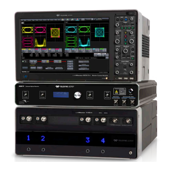
Operator’s Manual Introduction The Optical Modulation Analyzer (OMA) system combines the Teledyne LeCroy-Coherent Solutions coherent receiver with the LabMaster 10 Zi-A real-time oscilloscope. Taking advantage of the LabMaster’s high bandwidth and long acquisition memory, the coherent receiver enables high-speed and accurate characterization of complex optical modulations. -
Page 10: Shipped Items
Optical Modulation Analyzer Shipped Items Check that the following items have been included with your shipment. Contact Teledyne LeCroy immediately if any are missing. System Item Quantity MCM Zi-A Master Control Module Polarization Maintaining Patch Cord USB Type A to Type B Cable Operator’s Manual... -
Page 11: Coherent Receiver Features
Operator’s Manual Coherent Receiver Features 1. X Pol I RF output 12. USB connection to MCM-Zi-A 2. X Pol Q RF output 13. Mains power isolation switch 3. LCD control interface screen 14. AC power inlet (~100 - 240 V; 50/60 Hz; 20W max.) 4. -
Page 12: Labmaster Real-Time Oscilloscope
Coherent receiver, oscilloscope modules, and software may be purchased independently and combined to form an OMA system, although system performance may not equal that of a complete Teledyne LeCroy OMA system. The following hardware has been tested to be compatible with each other and the Optical LinQ OMA software. -
Page 13: Oma System Architecture
Operator’s Manual OMA System Architecture A modulated optical signal is input to the coherent receiver along with a Local Oscillator (LO). The coherent receiver also outputs a laser which can be used as a source for the LO. The output LO can be controlled from the coherent receiver’s LCD interface as well as from the OMA software. - Page 14 Optical Modulation Analyzer OMA system architecture with an emphasis on signal flow through the various components...
-
Page 15: Safety
Operator’s Manual Safety To maintain the OMA in a correct and safe condition, observe generally accepted safety procedures in addition to the precautions specified in this section. The overall safety of any system incorporating this product is the responsibility of the assembler of the system. Symbols These symbols appear on the instrument or in documentation to alert you to important safety concerns: CAUTION of potential damage to instrument, or WARNING of potential bodily injury. -
Page 16: Coherent Receiver Precautions
Optical Modulation Analyzer Use only power cords shipped with the instrument and certified for the country of use. Keep product surfaces clean and dry. Do not remove the covers or inside parts. Refer all maintenance to qualified personnel. Coherent Receiver Precautions Invisible Laser Radiation Exercise laser safety precautions. -
Page 17: Cooling
CAUTION Schedule an annual factory calibration as part of your regular maintenance. Extended warranty, calibration, and upgrade plans are available for purchase. Contact your Teledyne LeCroy sales representative or customersupport@teledynelecroy.com to purchase a service plan. The LabMaster software includes both automatic and user-initiated deskew calibration functions. -
Page 18: Power
Optical Modulation Analyzer Power LabMaster power ratings vary by model. If you are using LabMaster components other than those shipped as part of an OMA system, see the product datasheet at teledynelecroy.com for power ratings. Max. Consumption Component AC Power Source* (all accessories installed) Standby Consumption 100 to 240 VAC (±10%) at... -
Page 19: System Installation
Operator’s Manual System Installation Hardware Configuration The OMA has been designed to accommodate your preferred system configuration, whether that is a bench-top or rack-mount arrangement. The dimensions and layout of the panel elements ensure user friendly integration. OMA components are heavy. Do not attempt these installation procedures without assistance. - Page 20 Optical Modulation Analyzer Rackmount Configuration The OMA may also be mounted in a standard 19-inch rack. Remove all cables attached to the instruments before attempting to mount the CAUTION units within the rack. ROVIDE Optional OMA rackmount kit (IQS-RACKMOUNT) and •...
- Page 21 Operator’s Manual Connect Power Connect mains power to the OMA components first to provide ground connection. Always use an AC outlet with a good ground connection. Always wear an anti-static wrist strap before handling electrical components and equipment. WARNING Ensure that all cable connections are made before powering on the instruments. CAUTION A red Mains Power switch is located on the back of the control module.
-
Page 22: Optical Configuration
Optical Modulation Analyzer Optical Configuration Typical dual-polarization optical configuration... - Page 23 Operator’s Manual Example Optical Configurations OLARIZATION BUILT OLARIZATION UPPLIED INGLE OLARIZATION UILT...
- Page 24 Optical Modulation Analyzer Connect Standard RF Cables Follow these instructions to connect the standard RF cables (IQSCABLES-SBW) to the acquisition module’s 2.92mm interfaces. The supplied RF cables are labeled 'XI', 'XQ', 'YI', and 'YQ'. Do not bend or deform the cables, as this will damage them. Connect cables as labeled. The cables are calibrated to perform within specification only when connected as labeled.
- Page 25 Operator’s Manual Connect High Bandwidth RF Cables The following instructions apply when connecting the coherent receiver to DBI-enabled LabMaster acquisition modules. The semi-rigid RF cables are labeled 'XI', 'XQ', 'YI', and 'YQ'. Do not bend the cables sharply; keep the cables’ curvature as large as possible. Connect cables as labeled.
- Page 26 Optical Modulation Analyzer Your system should look similar to this: Connect Optical Signals Teledyne LeCroy coherent receivers utilize good quality connectors in compliance with EIA- 455-21A standards. To keep connectors clean and in good condition, inspect them with a CAUTION fiber-inspection probe before connecting them.
- Page 27 Operator’s Manual LEAN PTICAL ULKHEAD ONNECTORS Inspect the instrument bulkhead using a fiber inspection microscope: If the bulkhead is clean, proceed to connecting your optical fiber. • If the bulkhead is dirty, clean it using the appropriate bulkhead cleaning tool for your •...
-
Page 28: Coherent Receiver Lcd Control Interface
Optical Modulation Analyzer Coherent Receiver LCD Control Interface The LCD Control Interface may be used to manually set and configure the optical characteristics of the coherent receiver’s Internal Local Oscillator output. NOTE: The Internal Local Oscillator is automatically controlled from the OMA software when the coherent receiver is connected to the LabMaster and the system is powered on. -
Page 29: Changing Step Size
Operator’s Manual Changing Step Size Follow this procedure to change the step size (the increment increase) of the laser frequency or wavelength. 1. Turn the dial to select the ‘SETTINGS’ menu, then press. 2. Turn the dial to select the ‘STEP SIZE’ menu, then press. 3. -
Page 30: Preparing For Optimal Measurements
Optical Modulation Analyzer Preparing for Optimal Measurements The following procedures will prepare the oscilloscope to yield the most accurate measurements. We highly recommend performing each of them before starting an OMA test session. Warm Up Power on all components and allow them to warm for at least 20 min. before starting a test session. Deskew Channels The LabMaster oscilloscope has several self-calibration functions to correct for skew between channels. -
Page 31: Adjust Signal Pre-Processing
Operator’s Manual Adjust Signal Pre-Processing These Pre-processing settings on the Channel setup dialog affect pre-acquisition processes that will affect the waveform, such as noise filtering and interpolation. Channel Pre-processing settings Interpolation The LabMaster takes discrete signal samples which are then joined to show a continuous waveform trace. -
Page 32: Using The Optical Modulation Analyzer Software
Using the Optical Modulation Analyzer Software Starting the OMA Software Optical LinQ, Teledyne LeCroy’s optical modulation analysis software, is fully integrated into the LabMaster X-Stream firmware application. It can be started by choosing Analysis->OMA from the LabMaster touch screen menu bar. -
Page 33: Acquisition Controls
Operator’s Manual The OMA dialog is divided into the following control groups: A. Acquisition controls allow you to make signal acquisition settings and control the acquisition trigger from within the OMA dialog. B. OMA workflow buttons show the general OMA process and open the configuration subdialogs belonging to each phase. -
Page 34: Optical Inputs
Optical Modulation Analyzer Optical Inputs Touch the Optical Inputs workflow button to access the OMA’s optical configuration dialogs. Optical Inputs This subdialog is used to select the optical level parameters of the signal under test. NOTE: The OMA software will perform a calibration every time it detects changes in its settings. However, if there are changes on the transmitter side (such as output power change), then a manual calibration (Force Calibration) may be required for better signal characterization. - Page 35 Operator’s Manual Custom Modulation Upon selecting Custom Modulation Type, a new Symbol Definition dialog will appear. Use the Symbol Definition dialog to enter symbol definitions (QPSK example shown below). Control Action Edit Symbols Opens the Symbol Editor. Load From File Allows you to browse to and load a previously saved symbol file.
- Page 36 Optical Modulation Analyzer Internal Laser The Internal Laser dialog can be used to control the internal laser output. This dialog performs the same functions as the coherent receiver LCD Control Interface (p.20); it is added for convenience and remote control applications. NOTE: The coherent receiver’s internal laser measures its own output power.
-
Page 37: Electrical Inputs
The Coherent Receiver dialog is used to select the calibration script used by the receiver. If using a Teledyne LeCroy IQSxx or a legacy Coherent Solutions IQScope-RT, select IQScope. The IQScope Connected status checkbox will turn green when the software detects an IQScope via USB interface. - Page 38 Optical Modulation Analyzer USTOM OHERENT ECEIVER ALIBRATION CRIPT XAMPLE ; Custom Coherent Receiver .crs file ; Coherent Solutions 2014 ; Notes: ; Each float in the following must be specified in not more than 4 decimal places. ; Units have been selected so that there is no need for directly specifying very ;...
- Page 39 Operator’s Manual ; Units ; Type = Real array ; Range = -1e12 to 1e12 ; Default = 1,1,1,1,1,1,1,1,1,1,1,1,1,1,1,1,1,1,1,1,1,1,1,1,1,1,1,1,1,1 ; Max size of the array = 1024 (1K) XiMagnitude=1,1,1,1,1,1,1,1,1,1,1,1,1,1,1,1,1,1,1,1,1,1,1,1,1,1,1,1,1,1 XqMagnitude=1,1,1,1,1,1,1,1,1,1,1,1,1,1,1,1,1,1,1,1,1,1,1,1,1,1,1,1,1,1 YiMagnitude=1,1,1,1,1,1,1,1,1,1,1,1,1,1,1,1,1,1,1,1,1,1,1,1,1,1,1,1,1,1 YqMagnitude=1,1,1,1,1,1,1,1,1,1,1,1,1,1,1,1,1,1,1,1,1,1,1,1,1,1,1,1,1,1 ; Units = radians ; Type = Float array ;...
-
Page 40: Signal Processing
Optical Modulation Analyzer Signal Processing The Signal Processing dialog group is used to select the algorithms and their parameters to be applied at each stage of the optical signal processing. Touch the Signal Processing workflow button to access this group. See Using Custom MATLAB Scripts on p.50 for details on using custom algorithms. - Page 41 Operator’s Manual Pre-processor Parameters (Pre. Filter) This is the first stage in the DSP chain. You can use a range of built-in filters to improve signal quality or apply a custom algorithm via MATLAB . There is also a None option that can be used to bypass this processing stage.
- Page 42 Optical Modulation Analyzer When the Custom filter option is selected, the Pre. Custom subdialog is displayed. Click Edit Code to open the MATLAB editor and input your algorithm. More information can be found in Using Custom MATLAB Scripts on p.50.
- Page 43 Operator’s Manual Dispersion Compensation Parameters (Disp..) Use the Disp… subdialog to specify the parameters for the selected dispersion compensation algorithm. Control Action Fiber Length Sets length of the optic fiber in meters. Chromatic Dispersion Sets chromatic dispersion of the fiber in s/m2. Displays the product of the above two parameters or can be used to Total Dispersion directly specify the value.
- Page 44 Optical Modulation Analyzer Carrier Recovery Parameters (Carrier Rec. …) Use the Carrier Recovery subdialog to specify parameters for the Carrier Recovery algorithm. Two built-in methods are provided for selection on the DSP subdialog. The first is a modified Viterbi & Viterbi algorithm. Here, we first estimate frequency offset, which is then applied to the signal.
- Page 45 Operator’s Manual Post-processor Filter Parameters (Post. Filter) This is similar to the Pre-processor stage (p.33) where a range of built-in filters can be selected. You can input a custom algorithm via MATLAB or set to None to simply bypass.
- Page 46 Optical Modulation Analyzer Equalizer Parameters (Equalizer) The purpose of the equalizer is to correct frequency dependent distortion in the signal. It is an adaptive Finite Impulse Response (FIR). Similar to the other stages you can add a Custom algorithm via MATLAB or set it to None.
-
Page 47: Graphs
Operator’s Manual Graphs The Graphs functions allow you to control the display of several important time and frequency domain visualizations. The visualizations are divided into three categories for ease of use: Traces, IQ, and Eyes. Touch the button to open the configuration dialogs for that category. Visualizations from all three categories can be displayed simultaneously, as shown below. - Page 48 Optical Modulation Analyzer OMA display with 3D color persistence applied to highlight more frequently occurring samples...
- Page 49 Operator’s Manual Traces This set of visualizations shows time domain behavior of the input signals. The LabMaster Math functions allow further processing of the OMA trace data. See Applying Math Functions on p.52. RACE ISPLAY When in Single mode (selected at top-right corner of the menu bar), X and Y pols are each displayed in different tabs, as shown here: In Mosaic mode these tabs are shown side by side:...
- Page 50 Optical Modulation Analyzer RACE ELECTION Each trace can be turned on or off individually. The Traces dialogs also allow the display of S1-S3 polarization data as well as RAW traces and calibration buffers output from the acquisition unit. The various trace selection dialogs Dialog Trace Selector Shows...
- Page 51 Operator’s Manual Touch the I-Q button to turn on/off Trajectory and Constellation diagrams. As with traces, these diagrams can be shown in Mosaic mode or Single mode. Constellation diagrams for a QPSK dual-Pol signal arranged in mosaic mode The Scale Factor on the I-Q dialog controls how much area will be occupied by the plot inside the window.
- Page 52 Optical Modulation Analyzer Eyes Several eye diagrams are supported. Touch the Eyes button, then select the eye diagrams to compute from the Eyes subdialog. I and Q eye diagrams for a QPSK dual-Pol signal arranged in mosaic mode The Scale Factor controls how much area will be occupied by the plot inside the window. This is the same variable as for the I-Q plots and changing it will change their scale, too, and vice versa.
-
Page 53: Measurements
Operator’s Manual Measurements Measurements allow you to access key metrics of interest in tabular form. When turned on, OMA measurements appear immediately below the display grid. Each measurement can be enabled/disabled separately. Up-to-12 measurements can be enabled at once. Touch the Parameters button, then select from the Measurements and Meas. PolDeMux subdialogs. Parameters These commonly used optical parameters can be measured on OMA traces. - Page 54 Optical Modulation Analyzer Measurement Shows IQ Offset Center of the constellation with reference to the ideal center point, presented as a percentage. IQ RF Imbalance Ratio of the In-phase component versus the Quadrature component of the constellation points, presented as a percentage. Frequency Offset Frequency difference between the Transmitter laser and the OMA Local Oscillator.
- Page 55 Operator’s Manual Bit Error Rate (BER) After the input signals are digitally processed, the OMA can create the bit stream that was optically modulated. This bit-stream can be viewed on the touch screen display grid (as a trace) or saved to a file for further analysis.
- Page 56 Optical Modulation Analyzer YMBOL NCODING The OMA comes with a set of built-in encodings for the various modulation formats. Details of these can be found in Appendix 4: Reference Symbols and Encodings on p.73. Custom BER encoding defined through Optical LinQ software. You may input a Custom symbol-to-code map.
- Page 57 Operator’s Manual ATTERN ELECTION Use the Pattern Selection subdialog to specify the pattern that comprises the incoming bit stream. A range of polynomials can be selected, as well as Custom patterns. Each output stream requires its pattern to be specified. RROR Once patterns mapping and selection has been performed, the results can be seen on the Bit Error Rate subdialog.
-
Page 58: Using Custom Matlab Scripts
Optical Modulation Analyzer Using Custom MATLAB Scripts The OMA user interface allows you to select custom algorithms specified in MATLAB for numerous processing functions. NOTE: You must have MATLAB installed and running on the LabMaster in order to utilize custom algorithms. -
Page 59: Using X-Stream Browser
Operator’s Manual Using X-Stream Browser The LabMaster is installed with an application called X-Stream Browser™ that can be used to access data that may not be shown on the OMA dialogs: for example, DSP tap values, as shown below. To open X- Stream Browser: 1. -
Page 60: Applying Math And Measurements To Oma Data
Optical Modulation Analyzer Applying Math and Measurements to OMA Data The OMA functions are completely integrated with the other LabMaster functions, allowing you to apply extensive analysis features to OMA data. See the LabMaster 10 Zi-A Operator’s Manual for instructions on using Math and Measurement features. Applying Math Functions The LabMaster Math functions can be operated on any of the OMA’s data outputs. -
Page 61: Applying Measurements
Operator’s Manual Applying Measurements Any of the LabMaster measurements can also be applied to any of the OMA’s data outputs. There are 12 parameter slots available to use (P1 – P12). Measurements are added to a tabular display immediately below the waveform grids. Choose Measure >... -
Page 62: Maintenance
Optical Modulation Analyzer Maintenance Troubleshooting The OMA can fail to display results if not configured correctly. Warning and error messages are shown in red at bottom of the LabMaster touch screen display. While these messages are self-explanatory, two common errors are discussed below to assist you with troubleshooting. “OMA module not found!”... -
Page 63: Technical Support
Teledyne LeCroy publishes a free Technical Library on its website. Manuals, tutorials, application notes, white papers, and videos are available to help you get the most out of your Teledyne LeCroy products. The Datasheet published on the product page contains the detailed product specifications. Oscilloscope System Recovery Tools and Procedures contains instructions for using the Acronis®... -
Page 64: Returning A Product
4. Pack the product case in a cardboard shipping box with adequate padding to avoid damage in transit. 5. Mark the outside of the box with the shipping address given to you by Teledyne LeCroy. Be sure to add the following: ATTN: <RMA code assigned by Teledyne LeCroy>... -
Page 65: Warranty
The product is warranted for normal use and operation, within specifications, for a period of three years from shipment. Teledyne LeCroy will either repair or, at our option, replace any product returned to one of our authorized service centers within this period. However, in order to do this we must first examine the product and find that it is defective due to workmanship or materials and not due to misuse, neglect, accident, or abnormal conditions or operation. -
Page 66: Certifications
Optical Modulation Analyzer Certifications Teledyne LeCroy certifies compliance to the following standards as of the time of publication. See the EC Declaration of Conformity shipped with your product for the current certifications. EMC Compliance EC D - EMC ECLARATION OF... - Page 67 Operator’s Manual & N – EMC USTRALIA EALAND ECLARATION OF ONFORMITY The Optical Modulation Analyzer system complies with the EMC provision of the Radio Communications Act per the following standards, in accordance with requirements imposed by Australian Communication and Media Authority (ACMA): AS/NZS CISPR 11:2011 Radiated and Conducted Emissions, Group 1, Class A.
- Page 68 The instruments are subject to disposal and recycling regulations that vary by country and region. Many countries prohibit the disposal of waste electronic equipment in standard waste receptacles. For more information about proper disposal and recycling of your Teledyne LeCroy product, please visit teledynelecroy.com/recycle. ESTRICTION OF AZARDOUS...
-
Page 69: Appendix 1: Oma Calibration
Operator’s Manual Appendix 1: OMA Calibration The OMA system is calibrated at various stages to enable highly accurate signal measurements. Coherent Receiver Factory Calibrations Skew between output channels of the coherent receiver including external cables • Frequency Response of the coherent receiver •... -
Page 70: Appendix 2: Oma Algorithms
Optical Modulation Analyzer Appendix 2: OMA Algorithms Dispersion Compensation Dispersion is the process by which the different EM waves in the fiber travel at different speeds. The dispersion can originate from various different sources, such as material dispersion, waveguide dispersion, modal dispersion and polarization mode dispersion. Chromatic dispersion refers to the effect where different wavelengths travel at different speeds. -
Page 71: Polarization De-Multiplexing
Operator’s Manual Polarization De-multiplexing The term polarization refers to the directional plane that the Electromagnetic (EM) wave (carrier wave) oscillates in. Two EM waves can be made to propagate along the same fiber by combining them with a 90 degree difference in polarization (orthogonal polarization states or modes, A and A ). -
Page 72: Frequency Estimation
Optical Modulation Analyzer Constant amplitude for all four symbols OMA parameters for polarization de-multiplexing Frequency Estimation Since the OMA is based on Heterodyne Detection (Laser on Transmitter is not exactly the same laser on IQScope-RT), there will be a small frequency offset between the lasers. The frequency offset results in the rotation of the constellation plot. -
Page 73: Phase Estimation
Operator’s Manual Phase Estimation Lasers are not spectrally pure and they have random phase noise that needs to be corrected. The phase estimate technique commonly used in wireless transmission is called “Viterbi & Viterbi”. It finds the average phase error between an ideal symbol on a group of symbols and corrects for it. If the number of symbols is too low, you will get over-correction. -
Page 74: Appendix 3: Oma Measurement Definitions
Optical Modulation Analyzer Appendix 3: OMA Measurement Definitions I and Q Bias Offset The bias offset is a measure of how far the center of the constellation is with respect to the ideal center point. For QPSK and QAM modulation formats, the ideal center point is [0, 0] (I, Q). It is more convenient to represent the bias errors in percentages since this makes it independent of the average optical power. -
Page 75: Iq Offset
Operator’s Manual IQ Offset The IQ Offset is the shift in the center of the constellation points from the ideal location and is represented by the length of the Center vector as shown in the figure above. IQ Quadrature Error The quadrature error is a measure of the phase error of the constellation points with respect to the ideal phase relationship between the constellation points. -
Page 76: Iq Skew
Optical Modulation Analyzer IQ Skew The IQ skew is a measure of the time difference between the in-phase and quadrature crossing points in the eye diagrams as shown below. Equation 3 - Skew timing calculation Eye diagrams of QPSK signal skew... -
Page 77: Iq Rf Imbalance
Operator’s Manual IQ RF Imbalance The IQ RF imbalance is the ratio of the In-phase component versus the Quadrature component of the constellation points. The ratio is represented as a percentage, so 10% IQ RF imbalance would mean that the In-phase component is 10% larger than the Quadrature component. Equation 4 - IQ RF imbalance calculation IQ RF imbalance for QPSK... -
Page 78: Error Vector Magnitude
Optical Modulation Analyzer Error Vector Magnitude The error vector magnitude is the magnitude of the error vector, which is the difference between the signal vector and the ideal reference vector. It is more convenient to represent the EVM as a percentage such that it is unaffected by the average signal power (Equation 5). -
Page 79: Magnitude Error
Operator’s Manual Magnitude Error The magnitude error is the difference in amplitude between the reference symbol and the signal vector, as shown in Equation 6. The numerical value displayed as Magnitude Error in the software is the RMS of all the symbols captured during that acquisition. -
Page 80: Pdl
Optical Modulation Analyzer The Polarization Dependent Loss is calculated within the Polarization Demultiplexing Algorithm and its value is presented in dB. The resolution of this measurement is determined by the number of samples per | max (������������ ) | + | max (������������ baud. -
Page 81: Appendix 4: Reference Symbols And Encodings
Operator’s Manual Appendix 4: Reference Symbols and Encodings NOTE: The symbol values shown in the following table are normalized. When specifying custom symbols, you do not need to normalize the values as the OMA will do it automatically. Modulation = On Off Keying (bitsPerSymbol=1) Index Symbol Encoding... - Page 82 Optical Modulation Analyzer Modulation = 8QAM (bitsPerSymbol=3) Index Symbol Encoding Binary Gray1 Gray2 0.577+ 0.577i -0.577 + 0.577i -0.577- 0.577i 0.577 - 0.577i 1.155+0i -1.155 + 0i 0 + 1.155i 0 - 1.155i Modulation = 16QAM (bitsPerSymbol=4) Index Symbol Encoding Binary Gray1 Gray2...
- Page 83 Operator’s Manual Modulation = 32QAM (bitsPerSymbol=4) Index Symbol Encoding Binary Gray1 Gray2 -0.2234 - 0.2234i 01110 0.2234 - 0.2234i 10010 0.2234 + 0.2234i 10001 -0.2234 + 0.2234i 01101 -0.6708 - 0.2234i 01010 -0.2234 - 0.6708i 01111 0.2234 - 0.6708i 10011 0.6708 - 0.2234i 10110 0.6708 + 0.2234i...
- Page 84 Optical Modulation Analyzer Modulation = 64QAM (bitsPerSymbol=5) Index Symbol Encoding Binary Gray 1 Gray 2 -0.1543 - 0.1543i 011011 010010 0.1543 - 0.1543i 100011 110010 0.1543 + 0.1543i 100100 110110 -0.1543 + 0.1543i 011100 010110 -0.4630 - 0.1543i 010011 011010 -0.1543 - 0.4630i 011010 010011...
- Page 85 Operator’s Manual Modulation = 64QAM (bitsPerSymbol=5) -0.7715 - 0.7715i 001001 001001 -0.1543 - 1.0801i 011000 010000 0.1543 - 1.0801i 100000 110000 0.7715 - 0.7715i 110001 101001 1.0801 - 0.1543i 111011 100010 1.0801 + 0.1543i 111100 100110 0.7715 + 0.7715i 110110 101101 0.1543 + 1.0801i 100111...
- Page 86 Optical Modulation Analyzer...
- Page 88 927295-00 Rev A August, 2016...
Need help?
Do you have a question about the LabMaster LM 10-25Zi-A and is the answer not in the manual?
Questions and answers