Page 1 1-Port VNA Series R140 R180/RP180 Operating Manual Software version 18.3.0 July 2018...
Page 2: Table Of Contents
2.4 Test Port ............................. 23 2.5 Mini B USB Port ..........................23 2.6 External Trigger Signal Input Connector (R140 model only) ........24 2.7 External Reference Frequency Input Connector (R140 model only) ......24 2.8 Reference Frequency Input/Output Connector (R60 and R180 model only) 24 2.9 External Trigger Signal Input/Output Connector (R60 and R180 model...
Page 3 4.6.1.2 External Trigger Polarity ....................71 4.6.1.3 External Trigger Position ..................... 72 4.6.1.4 External Trigger Delay ....................73 4.6.2 Trigger Output (except R54/R140) .................. 76 4.6.2.1 Switching ON/OFF Trigger Output ................77 4.6.2.2 Trigger Output Polarity ....................78 4.6.2.3 Trigger Output Function ....................79 4.7 Scale Setting .............................
Page 4 4.8.3 Sweep Points Setting ......................87 4.8.4 Stimulus Power Setting ......................88 4.8.5 Segment Table Editing ......................88 4.9 Trigger Setting ..........................91 4.10 Measurement Optimizing ......................92 4.10.1 IF Bandwidth Setting ......................92 4.10.2 Averaging Setting ......................... 92 4.10.3 Smoothing Setting ....................... 93 4.10.4 Trace Hold Function ......................
Page 5 5.3.4 Calibration Standard Editing .................... 124 5.3.5 Calibration Standard Defining by S-Parameter File ..........126 5.4 Automatic Calibration Module ....................128 5.4.1 Automatic Calibration Module Features ..............129 5.4.2 Automatic Calibration Procedure ................... 130 6. MEASUREMENT DATA ANALYSIS ................. 131 6.1 Markers .............................
Page 6 6.5.1 Time Domain Gate Activating ..................178 6.5.2 Time Domain Gate Span..................... 178 6.5.3 Time Domain Gate Type ..................... 179 6.5.4 Time Domain Gate Shape Setting .................. 179 6.6 S-Parameter Conversion ......................180 6.7 Limit Test ............................182 6.7.1 Limit Line Editing ......................... 183 6.7.2 Limit Test Enabling/Disabling ..................
Page 7 10.5 Frequency adjustment of the internal generators ............214 10.5.1 Manual frequency adjustment ..................215 10.5.2 Automatic frequency adjustment ................. 215 10.6 Features of analyzers calibration ..................216 10.6.1 Calibration Type ........................217 10.6.2 Scalar Transmission Normalization................218 10.6.3 Expanded Transmission Normalization ..............218 10.7 Selection of the measured S-parameters .................
Page 8: Introduction
INTRODUCTION This Operating Manual represents design, specifications, overview of functions, and detailed operation procedure for the Vector Network Analyzer, to ensure effective and safe use of the technical capabilities of the instrument by the user. Vector Network Analyzer operation and maintenance should be performed by qualified engineers with initial experience in operating of microwave circuits and The following abbreviations are used in this Manual: PC –...
Page 9: Safety Instructions
III, or IV device. The Analyzer is tested in stand-alone condition or in combination with the accessories supplied by Copper Mountain Technologies against the requirement of the standards described in the Declaration of Conformity. If it is used as a system component, compliance of related regulations and safety requirements are to be confirmed by the builder of the system.
Page 10 SAFETY INSTRUCTIONS CAUTION This sign denotes a hazard. It calls attention to a procedure, practice or condition that, if not correctly performed or adhered to, could result in damage to or destruction of part or all of the instrument. Note This sign denotes important information.
Page 11: General Overview
1. GENERAL OVERVIEW 1.1 Description The VNA is designed for use in the process of development, adjustment and testing of antenna-feeder devices in industrial and laboratory facilities, as well as in field, including operation as a component of an automated measurement system. The Analyzer is designed for operation with external PC, which is not supplied with it.
Page 12 GENERAL OVERVIEW Segment sweep A frequency sweep within several user-defined segments. Frequency range, number of sweep points, IF bandwidth and measurement delay should be set for each segment. Power settings Two modes of output power level. Power levels depending on device. Sweep trigger Trigger modes: continuous, single, hold.
Page 13 GENERAL OVERVIEW Factory calibration The factory calibration of the Analyzer allows performing measurements without additional calibration and reduces the measurement error after reflection normalization. Mechanical The user can select one of the predefined calibration kits calibration kits of various manufacturers or define own calibration kits. Electronic calibration Electronic calibration modules manufactured by COPPER modules...
Page 14 GENERAL OVERVIEW Statistics Calculation and display of mean, standard deviation and peak-to-peak in a frequency range limited by two markers on a trace. Bandwidth Determines bandwidth between cutoff frequency points for an active marker or absolute maximum. The bandwidth value, center frequency, lower frequency, higher frequency, Q value, and insertion loss are displayed.
Page 15 GENERAL OVERVIEW Time domain The function performs data transformation from transformation frequency domain into response of the DUT to radiopulse in time domain. Time domain span is set by the user arbitrarily from zero to maximum, which is determined by the frequency step. Windows of various forms allow better tradeoff between resolution and level of spurious sidelobes.
Page 16: Principle Of Operation
GENERAL OVERVIEW 1.4 Principle of Operation The Analyzer consists of the Analyzer Unit, some supplementary accessories, and personal computer (which is not supplied with the package). The Analyzer Unit is powered and controlled by PC via USB-interface. The block diagram of the Analyzer is represented in Figure 1.1.
Page 17 Figure 1.1The VNA block diagram...
Page 18: Preparation For Use
2. PREPARATION FOR USE 2.1 General Information Unpack the VNA and other accessories. Connect the Analyzer to the PC using the USB Cable supplied in the package. Install the software (supplied on the flash drive) onto your PC. The software installation procedure is described below.
Page 19 PREPARATION FOR USE To avoid motherboard damage you must use USB cables supplied in the package or similar ones according to the Attention! specifications shown in Figure 2.1 and Figure 2.2 (for R180/RP180 only) Figure 2.1 USB TYPE C TO C 2.0, 3A Figure 2.2 USB TYPE C TO USB 2.0 A MALE, 3A...
Page 20: Software Installation
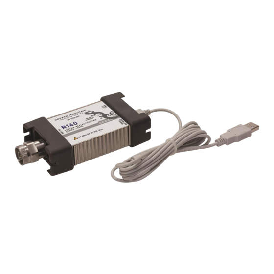
PREPARATION FOR USE 2.2 Software Installation The software is installed to the external PC running under Windows operating system. The Analyzer is connected to the external PC via USB interface. Minimal system WINDOWS 2000/XP/VISTA/7/8 requirements for 1.5 GHz Processor the PC 2 GB RAM USB 2.0 High Speed The supplied USB flash drive contains the following software:...
Page 21  green blinking light – standby mode. In this mode the current consumption of the device from the USB port is minimum;  green glowing light – normal device operation. Figure 2.3 R140 top panel Figure 2.4 R54 top panel Figure 2.5 R60 top panel...
Page 22 PREPARATION FOR USE Figure 2.6 R180 top panel...
Page 23: Test Port
The mini B USB port view is represented in Figure 2.7, Figure 2.8, Figure 2.9 and Figure 2.10. It is intended for connection to USB port of the personal computer via the supplied USB cable. Figure 2.7 Mini B USB port R54 Figure 2.8 Mini B USB port R140...
Page 24: External Trigger Signal Input Connector (R140 Model Only)
Figure 2.9 Mini B USB port R60 Figure 2.10 Mini B USB port R180 2.6 External Trigger Signal Input Connector (R140 model only) This connector allows the user to connect an external trigger source. Connector type is SMA female. TTL compatible inputs of 3 V to 5 V magnitude have up to 1 us pulse width.
Page 25: External Trigger Signal Input/Output Connector (R60 And R180 Model Only)
PREPARATION FOR USE 2.9 External Trigger Signal Input/Output Connector (R60 and R180 model only) External Trigger Signal Input allows the user to connect an external trigger source. Connector type is SMA female. 3.3v CMOS TTL compatible inputs magnitude have at least 1 μs pulse width. Input impedance is at least 10 kOhm. The External Trigger Signal Output port can be used to provide trigger to an external device.
Page 26: Getting Started
3. GETTING STARTED This section represents a sample session of the Analyzer. It describes the main techniques of measurement of reflection coefficient parameters of the DUT. SWR and reflection coefficient phase of the DUT will be analyzed. The instrument sends the stimulus to the input of the DUT and then receives the reflected wave.
Page 27: Analyzer Preparation For Reflection Measurement
GETTING STARTED 3.1 Analyzer Preparation for Reflection Measurement Turn on the Analyzer and warm it up for the period of time stated in the specifications. Ready state The bottom line of the screen displays the instrument status features bar. It should read Ready. Connect the DUT to the test port of the Analyzer.
Page 28: Stimulus Setting
GETTING STARTED 3.3 Stimulus Setting After you have restored the preset state of the Analyzer, the stimulus parameters will be as follows: full frequency range of the instrument, sweep type is linear, number of sweep points is 201, power level is high, and IF is 10 kHz. For the current example, set the frequency range from 100 MHz to 1 GHz.
Page 29: If Bandwidth Setting
GETTING STARTED 3.4 IF Bandwidth Setting For the current example, set the IF bandwidth to 3 kHz. To set the IF bandwidth to 3 kHz use the following softkey in the left menu bar Average. Then select the IFBW field in the Average dialog. To set the IF bandwidth in the IFBW dialog use the following softkeys 3 kHz >...
Page 30: Number Of Traces, Measured Parameter And Display Format Setting
GETTING STARTED 3.5 Number of Traces, Measured Parameter and Display Format Setting In the current example, two traces are used for simultaneous display of the two parameters (SWR and reflection coefficient phase). To add the second trace use the following softkeys in the right menu bar Trace > Add trace.
Page 31: Trace Scale Setting
GETTING STARTED To select the first trace display format click on Active Trace and on Format. In the Format dialog use the following softkeys SWR > Ok. Close the dialogs by Ok. 3.6 Trace Scale Setting For a convenience in operation, change the trace scale using automatic scaling function.
Page 32 GETTING STARTED To perform full 1-port calibration, you need to prepare the kit of calibration standards: OPEN, SHORT and LOAD. Every kit has its description and specifications of the standards. To perform proper calibration, you need to select the correct kit type in the program.
Page 33 GETTING STARTED Then select the required kit from the Calibration Kits list and complete the setting by Ok. To perform full 1-port calibration you should execute measurements of the three standards. After that the table of calibration coefficients will be calculated and saved into the memory of the Analyzer.
Page 34: Swr And Reflection Coefficient Phase Analysis Using Markers
GETTING STARTED Connect an OPEN standard and click Open. Connect a SHORT standard and click Short. Connect a LOAD standard and click Load. After clicking any of the Open, Short, or Load softkeys, wait until the calibration procedure is completed. To complete the calibration and calculate the table of calibration coefficients click Apply.
Page 35 GETTING STARTED Figure 3.3 SWR and reflection coefficient phase measurement example To enable a new marker use the following softkeys in the left menu bar Marker > Add Marker. Double click on the marker in the Marker List to activate the on-screen keypad and enter the marker frequency value.
Page 36: Measurement Conditions Setting
4. MEASUREMENT CONDITIONS SETTING 4.1 Screen Layout and Functions The screen layout is represented in Figure 4.1. In this section you will find detailed description of the softkey menu bars and instrument status bar. The channel windows will be described in the next section. Figure 4.1 Analyzer screen layout 4.1.1 Left and Right Softkey Menu Bars The softkey menu bars in the left and right parts of the screen are the main menu...
Page 37: Top Menu Bar
MEASUREMENT CONDITIONS SETTING On-screen alphanumeric keypads also support data entering from external PC keyboard. Besides, you can navigate the menu by «Up Arrow», «Down Arrow»,«Enter», «Esc» keys on the external keyboard. To expand the menu bar click on it and drag the cursor to the right or to the left accordingly.
Page 38 MEASUREMENT CONDITIONS SETTING The softkey Save Data allows to save the trace data in CSV format (see section 8.3.1). The softkeys Add Marker and Delete Marker add and delete markers on the trace respectively. The softkey Reference Marker allows to add the reference marker on the trace. To delete the reference marker reclick this key.
Page 39 MEASUREMENT CONDITIONS SETTING The softkey Data Math pops up the corresponding dialog form for choosing the math operation type between data traces and memory traces (see section 6.2.4). The softkey Auto Scale allows to define the trace scale automatically so that the trace of the measured value could fit into the graph entirely (see section 3.6).
Page 40: Instrument Status Bar
MEASUREMENT CONDITIONS SETTING The softkey Inverse Color allows to change the interface color. 4.1.3 Instrument Status Bar Figure 4.2 Instrument status bar The instrument status bar is located at the bottom of the screen. It can contain the following messages (see Table 4.1). Table 4.1 Messages in the instrument status bar Field Message...
Page 41 MEASUREMENT CONDITIONS SETTING Field Message Instrument Status Description Error correction Correction Off Error correction disabled by the user status System System correction System correction disabled by the user. Correction Off status Disabling of error correction does not affect factory calibration.
Page 42: Channel Window Layout And Functions
MEASUREMENT CONDITIONS SETTING 4.2 Channel Window Layout and Functions The channel windows display the measurement results in the form of traces and numerical values. The screen can display up to 4 channel windows simultaneously. Each window has the following parameters: ...
Page 43: Channel Title Bar
MEASUREMENT CONDITIONS SETTING 4.2.1 Channel Title Bar The channel title feature allows you to enter your comment for each channel window. To show/hide the channel title bar use the softkey Display. Click on Caption field in the opened dialog. To edit the channel title click on the softkey Edit to recall the on- Note screen keypad.
Page 44 MEASUREMENT CONDITIONS SETTING The trace status field displays the name and parameters of a trace. The number of lines in the field depends on the number of traces in the channel. Using the trace status field you can easily modify the trace Note parameters by the mouse.
Page 45 MEASUREMENT CONDITIONS SETTING Table 4.2 Trace status symbols definition Status Symbols Definition OPEN response calibration Error Correction SHORT response calibration Full 1-port calibration Port impedance conversion De-embedding Data Analysis Embedding Port extension Data + Memory Data - Memory Math Operations Data * Memory Data / Memory Hold of the trace maximum between repeated...
Page 46: Graph Area
MEASUREMENT CONDITIONS SETTING Status Symbols Definition Data trace Trace display Memory trace D&M Data and memory traces Data and memory traces - off 4.2.3 Graph Area The graph area displays the traces and numeric data (see Figure 4.5). Figure 4.5 Graph area...
Page 47: Markers
MEASUREMENT CONDITIONS SETTING The graph area contains the following elements:  Vertical graticule label displays the vertical axis numeric data for the active trace;  Horizontal graticule label displays stimulus axis numeric data (frequency, time, or distance);  Reference level position indicates the reference level position of the trace; ...
Page 48: Channel Status Bar
MEASUREMENT CONDITIONS SETTING The markers are numbered from 1 to 16. The reference marker is indicated with R symbol. The active marker is indicated in the following manner: its number is highlighted in inverse color, the stimulus indicator is fully colored. 4.2.5 Channel Status Bar The channel status bar is located in the bottom part of the channel window (see Figure 4.7)
Page 49: Quick Channel Setting Using Mouse
This section describes the manipulations, which will enable you to set the channel parameters of R140 fast and easy. When you move a mouse pointer in the channel window field where a channel parameter can be changed, the mouse pointer will change its form and a prompt field will appear.
Page 50: Active Trace Selection
MEASUREMENT CONDITIONS SETTING 4.3.2 Active Trace Selection You can select the active trace if the active channel window contains two or more traces. The active trace name will be highlighted in inverted color. In the example given it is Tr2. To activate a trace click on the required trace or its status line. 4.3.3 Display Format Setting To select the trace display format click on the format name in the trace status line.
Page 51: Reference Level Setting
MEASUREMENT CONDITIONS SETTING To select the trace scale click in the trace scale field of the trace status line. Enter the required numerical value using the on-screen keypad and complete the setting by Ok. 4.3.5 Reference Level Setting To set the value of the reference level click on the reference level field in the trace status line.
Page 52: Marker Stimulus Value Setting
MEASUREMENT CONDITIONS SETTING 4.3.6 Marker Stimulus Value Setting The marker stimulus value can be set by dragging the marker or by entering the value from the on-screen keypad. To drag the marker, move the mouse pointer to one of the marker indicators. The marker will become active, and a pop-up hint with its name will appear near the marker.
Page 53: Start/Center Value Setting
MEASUREMENT CONDITIONS SETTING 4.3.8 Start/Center Value Setting To enter the Start/Center numerical values click on the respective field in the channel status bar. Then enter the required value using the on-screen keypad. 4.3.9 Stop/Span Value Setting To enter the Stop/Span numerical values click on the respective field in the channel status bar.
Page 54: Sweep Points Number Setting
MEASUREMENT CONDITIONS SETTING 4.3.10 Sweep Points Number Setting To enter the number of sweep points click in the respective field of the channel status bar. Select the required value in the Points dialog and complete the setting by Ok. 4.3.11 IF Bandwidth Setting To set the IF bandwidth click in the respective field of the channel status bar.
Page 55: Power Level Setting
MEASUREMENT CONDITIONS SETTING 4.3.12 Power Level Setting To set the output power level click in the respective field of the channel status bar. This way you can switch between high and low power settings. 4.4 Channel and Trace Display Setting The Analyzer supports 4 channels, which allows measurements with different stimulus parameter settings.
Page 56: Channel Activating
MEASUREMENT CONDITIONS SETTING To set the number of channel windows displayed on the screen use the following softkey in the right menu bar Channels. Then select the softkey with the required number and layout of the channel windows. In the Active Channel field, you can select the active channel. The repeated clicking will switch the numbers of all channels.
Page 57: Active Channel Window Maximizing
MEASUREMENT CONDITIONS SETTING To activate the channel use the following softkeys in the right menu bar Channels > Active Channel. Active Channel field allows viewing the numbers of all channels from 1 to 4. Select the required number of the active channel. To activate a channel, you can also click on its channel window.
Page 58: Number Of Traces Setting
MEASUREMENT CONDITIONS SETTING To enable/disable active channel maximizing function use the following softkeys Channel > Maximize Channel. Channel maximizing function can be controlled by a double mouse Note click on the channel. 4.4.4 Number of Traces Setting Each channel window can contain up to 4 different traces. Each trace is assigned the display format, scale and other parameters.
Page 59: Active Trace Selection
MEASUREMENT CONDITIONS SETTING To add a trace use the following softkeys in the right menu bar Trace > Add Trace. To delete a trace use the following softkeys in the right menu bar Trace > Delete Trace. All the traces are assigned their individual names, which cannot be changed. The trace name contains its number.
Page 60 MEASUREMENT CONDITIONS SETTING To select the active trace use the softkeys in the right menu bar Trace. Click the Active Trace to select the trace you want to assign the active. A trace can be activated by clicking on the trace status bar in the Note graphical area of the program...
Page 61 MEASUREMENT CONDITIONS SETTING Table 4.4 Channel parameters Parameter Description Sweep Range Number of Sweep Points IF Bandwidth Table 4.5 Trace parameters Parameter Description Display Format Reference Level Scale, Value and Position Electrical Delay, Phase Offset Memory Trace Markers Parameter Transformation...
Page 62: Measurement Parameters Setting
Port incident wave Port R140 Analyzer has one measurement port which operates as a signal source and as a reflected signal receiver. That is why the Analyzer allows measuring only S11 parameter. 4.5.2 Trace Format The Analyzer offers the display of the measured S-parameters on the screen in three formats: ...
Page 63: Rectangular Format
MEASUREMENT CONDITIONS SETTING 4.5.3 Rectangular Format In this format, stimulus values are plotted along X-axis and the measured data are plotted along Y-axis (see Figure 4.10). Figure 4.10 Rectangular format To display S-parameter complex value along Y-axis, it should be transformed into a real number.
Page 64 MEASUREMENT CONDITIONS SETTING Format Type Measurement Unit Label Data Type (Y-axis) Description (Y-axis) Voltage Standing Abstract number Wave Ratio S-parameter phase from –180to +180 Phase Phase Degree (°)  arctg  S-parameter phase, Expanded Expand measurement range expanded Degree (°) Phase Phase to from below...
Page 65: Polar Format
MEASUREMENT CONDITIONS SETTING 4.5.4 Polar Format Polar format represents the measurement results on the pie chart (see Figure 4.11). The distance to a measured point from the graph center corresponds to the magnitude of its value. The counterclockwise angle from the positive horizontal axis corresponds to the phase of the measured value.
Page 66: Smith Chart Format
MEASUREMENT CONDITIONS SETTING 4.5.5 Smith Chart Format Smith chart format is used for representation of impedance values for DUT reflection measurements. In this format, the trace has the same points as in polar format. Figure 4.12 Smith chart format Smith chart format does not have a frequency axis, so frequency will be indicated by the markers.
Page 67 MEASUREMENT CONDITIONS SETTING Format Type Measurement Unit Data Displayed by Marker Label Description (Y-axis) Resistance at input: R  Ohm (Ω)    Reactance at input: Complex Smith X  Impedance Ohm (Ω) (R + jX) (at Input) Equivalent capacitance or inductance: ...
Page 68: Data Format Setting
MEASUREMENT CONDITIONS SETTING 4.5.6 Data Format Setting You can select the format for each trace of the channel individually. Before you set the format, first activate the trace. To set the trace display format use the following softkey in the right menu bar Trace.
Page 69: Trigger Setting
MEASUREMENT CONDITIONS SETTING 4.6 Trigger Setting The trigger mode determines the sweep actuation of the channel at a trigger signal detection. A channel can operate in one of the following three trigger modes:  Continuous – a sweep actuation occurs every time a trigger signal is detected;...
Page 70 MEASUREMENT CONDITIONS SETTING Then select the required trigger mode:  Hold  Single  Continuous To set the trigger source, use the following softkeys Trigger > Trigger Source. Then select the required trigger source:  Internal  External  Bus...
Page 71: External Trigger (Except R54)
MEASUREMENT CONDITIONS SETTING 4.6.1 External Trigger (except R54) 4.6.1.1 Point Feature By default the external trigger initiates a sweep measurement upon every trigger event (See Figure 4.13 a, b). For the external trigger source, the point trigger feature instead initiates a point measurement upon each trigger event (See Figure 4.13 c, d).
Page 72: External Trigger Position
MEASUREMENT CONDITIONS SETTING To select the external trigger polarity, use the following softkeys Trigger > Trigger Input > Polarity { NegativeEdge | Positive Edge }. 4.6.1.3 External Trigger Position The external trigger position selects the position when Analyzer expects the external trigger signal: ...
Page 73: External Trigger Delay
MEASUREMENT CONDITIONS SETTING To select external trigger polarity, use the following softkeys: Trigger > Trigger Input > Position { Before Sampling | Before Setup }. 4.6.1.4 External Trigger Delay The external trigger delay sets the response delay with respect to the external trigger signal (see Figure 4.13).
Page 74 MEASUREMENT CONDITIONS SETTING...
Page 75 MEASUREMENT CONDITIONS SETTING Figure 4.13 External Trigger...
Page 76: Trigger Output (Except R54/R140)
MEASUREMENT CONDITIONS SETTING 4.6.2 Trigger Output (except R54/R140) The trigger output outputs various waveforms depending on the setting of the Output Trigger Function:  Before frequency setup pulse;  Before sampling pulse;  After sampling pulse;  Ready for external trigger;...
Page 77: Switching On/Off Trigger Output
MEASUREMENT CONDITIONS SETTING 4.6.2.1 Switching ON/OFF Trigger Output To enable/disable the trigger output, use the following softkeys Trigger > Trigger Output > Enable Out. When the Ready for Trigger function of the trigger output is Note selected the trigger source must be set to external to enable the output trigger.
Page 78: Trigger Output Polarity
MEASUREMENT CONDITIONS SETTING 4.6.2.2 Trigger Output Polarity To select the polarity of the trigger output, use the following softkeys Trigger > Trigger Output > Polarity { NegativeEdge | Positive Edge }.
Page 79: Trigger Output Function
MEASUREMENT CONDITIONS SETTING 4.6.2.3 Trigger Output Function To select the function of the trigger output (See Figure 4.14, Figure 4.15), use the following softkeys Trigger > Trigger Output > Position { Before Setup | BeforeSampling | After Sampling | Ready for Trigger | Sweep End | Measurement }.
Page 80: Scale Setting
MEASUREMENT CONDITIONS SETTING 4.7 Scale Setting 4.7.1 Rectangular Scale For rectangular format you can set the following parameters (see Figure 4.16):  Trace scale;  Reference level value;  Reference level position;  Number of scale divisions. Figure 4.16 Rectangular scale 4.7.2 Rectangular Scale Setting You can set the scale for each trace of a channel.
Page 81: Circular Scale
MEASUREMENT CONDITIONS SETTING Then select the Scale field and enter the required value using the on-screen keypad. To set the reference level select the Ref. Value field and enter the required value using the on-screen keypad. To set the position of the reference level select the Ref. Position field and enter the required value using the on-screen keypad.
Page 82: Automatic Scaling
MEASUREMENT CONDITIONS SETTING To set the scale of the circular graph use the following softkey in the right menu bar Scale. Then select the Scale field and enter the required value using the on-screen keypad. 4.7.5 Automatic Scaling The automatic scaling function allows the user to define the trace scale automatically so that the trace of the measured value could fit into the graph entirely.
Page 83: Reference Level Automatic Selection
MEASUREMENT CONDITIONS SETTING 4.7.6 Reference Level Automatic Selection This function executes automatic selection of the reference level in rectangular coordinates. After the function has been executed, the trace of the measured value makes the vertical shift so that the reference level crosses the graph in the middle. The scale will remain the same.
Page 84: Phase Offset Setting
MEASUREMENT CONDITIONS SETTING The electrical delay is set for each trace individually. Before you set the electrical delay, first activate the trace. To set the electrical delay use the following softkey in the right menu bar Scale. Then select the Electrical Delay field and enter the required value using the on- screen keypad.
Page 85 MEASUREMENT CONDITIONS SETTING Then select the Phase Offset field and enter the required value using the on- screen keypad.
Page 86: Stimulus Setting
MEASUREMENT CONDITIONS SETTING 4.8 Stimulus Setting The stimulus parameters are set for each channel. Before you set the stimulus parameters of a channel, make this channel active. 4.8.1 Sweep Type Setting To set the sweep type use the following softkey in the right menu bar Stimulus. If you select segment frequency sweep, the Segment Table softkey Note will be become available in Stimulus dialog.
Page 87: Sweep Points Setting
MEASUREMENT CONDITIONS SETTING To enter the start and stop values of the sweep range use the following softkey in the right menu bar Stimulus. Then select the Start Frequency or Stop Frequency field and enter the required values using the on-screen keypad. If necessary, you can select the measurement units.
Page 88: Stimulus Power Setting
MEASUREMENT CONDITIONS SETTING Then click on Points field, select the required value from the list and complete the setting by Ok. 4.8.4 Stimulus Power Setting The stimulus power level can take two possible values. High output power corresponds to the source signal power of -10 dB/m. Low output power corresponds to -30 dBm.
Page 89 MEASUREMENT CONDITIONS SETTING The types of segment tables are shown below. Each table line determines one segment. The table can contain one or several lines. The number of lines is limited by the aggregate number of all segment points, i.e. 100001 To edit the segment table use the following softkeys in the right menu bar Stimulus >...
Page 90 MEASUREMENT CONDITIONS SETTING To enter the segment parameters, move the mouse to the respective box and enter the numerical value. You can navigate the segment table using the «Up Arrow», «Down Arrow », «Left Arrow », «Right Arrow» keys. Note The adjacent segments cannot overlap in the frequency domain.
Page 91: Trigger Setting
MEASUREMENT CONDITIONS SETTING 4.9 Trigger Setting The Analyzer can operate in one of three sweep trigger modes. The trigger mode determines the sweep actuation. The trigger can have the following modes:  Continuous – a sweep actuation occurs every time after sweep cycle is complete in each channel;...
Page 92: Measurement Optimizing
MEASUREMENT CONDITIONS SETTING 4.10 Measurement Optimizing 4.10.1 IF Bandwidth Setting The IF bandwidth function allows the user to define the bandwidth of the test receiver. The IF bandwidth can be selected by user from the following values: 100 Hz, 300 Hz, 1 kHz, 3 kHz, 10 kHz and 30 kHz. The IF bandwidth narrowing allows you to reduce self-noise and widen the dynamic range of the Analyzer.
Page 93: Smoothing Setting
MEASUREMENT CONDITIONS SETTING To set the averaging use the following softkey in the left menu bar Average. To toggle the averaging function on/off click on Average field. To set the averaging factor click on Averaging Factor field and enter the required value using the on-screen keypad.
Page 94 MEASUREMENT CONDITIONS SETTING To set the smoothing use the following softkey in the left menu bar Average. To toggle the smoothing function on/off click on Smoothing field. To set the smoothing aperture click on Smoothing Aperture field and enter the required value using the on-screen keypad.
Page 95: Trace Hold Function
MEASUREMENT CONDITIONS SETTING 4.10.4 Trace Hold Function The Trace Hold function displays the maximum or the minimum of any given active measurement instead the real-time data. The held data is displayed as an active trace. To toggle the Trace Hold function on/off use the following softkeys in the right menu bar Trace >...
Page 96: Cable Specifications
MEASUREMENT CONDITIONS SETTING 4.11 Cable Specifications By default, the program does NOT compensate DTF measurements to account for the inherent loss of a cable. However, to make more accurate DTF measurements, the cable loss and velocity factor can be entered using one of the following methods: ...
Page 97: Manually Specify Velocity Factor And Cable Loss
MEASUREMENT CONDITIONS SETTING Select the required item from the Cable List and complete the setting by Ok 4.11.2 Manually specify Velocity Factor and Cable Loss To set the parameters of cable, press the following softkeys in the left menu bar Analysis >...
Page 98: Editing Table Of Cables
MEASUREMENT CONDITIONS SETTING Click on Velocity Factor field to enter the value of velocity factor using the on- screen keypad. Click on Loss field to enter the value of cable loss using the on-screen keypad. 4.11.3 Editing table of cables To edit the table of cables, press the following softkeys in the left menu bar Analysis >...
Page 99 MEASUREMENT CONDITIONS SETTING Click the left button of the mouse on the field Cable Type. To add/delete rows in the table click Add/Delete. Then select the required parameter in the table and double click on the corresponding cell. Enter the required value Cable Name, Velocity, Cable Loss etc using the on-screen keypad.
Page 100: Calibration And Calibration Kit
5. CALIBRATION AND CALIBRATION KIT 5.1 General Information 5.1.1 Measurement Errors S-parameter measurements are influenced by various measurement errors, which can be devided into two categories:  systematic errors,  random errors. Random errors comprise such errors as noise fluctuations and thermal drift in electronic components, changes in the mechanical dimensions of connectors subject to temperature drift, repeatability of connections.
Page 101: Directivity Error
CALIBRATION AND CALIBRATION KIT The measurement results till the procedure of error correction has been executed are called uncorrected. The residual values of the measurement results after the procedure of error correction are called effective. 5.1.2.1 Directivity Error A directivity error (Ed) is caused by incomplete separation of the incident signal from the reflected signal by the directional coupler in the source port.
Page 102: Analyzer Test Port Defining
CALIBRATION AND CALIBRATION KIT Figure 5.1 One-port error model Where: – reflection coefficient true value; – reflection coefficient measured value. The measurement result at test port is affected by the following three systematic error terms: – directivity; – source match; –...
Page 103: Calibration Steps
CALIBRATION AND CALIBRATION KIT Sometimes it is necessary to connect coaxial cable and/or adapter to the connector on the front panel for connection of the DUT with a different connector type. In such cases connect calibration standards to the connector of the cable or adapter.
Page 104: Calibration Methods
CALIBRATION AND CALIBRATION KIT Calibration is applied to the Analyzers channel. This means that the table of calibration coefficients is being stored for the channel. 5.1.6 Calibration Methods The Analyzer supports several methods of calibration. The calibration methods vary by quantity and type of the standards being used, by type of error correction. The Table 5.1 represents the overview of the calibration methods.
Page 105: Expanded Normalization
CALIBRATION AND CALIBRATION KIT 5.1.6.2 Expanded Normalization Expanded normalization involves connection of the following two standards to the test port:  SHORT or OPEN, and  LOAD. Measurement of the two standards allows for estimation of the reflection tracking error term Er and directivity error term – Ed. 5.1.6.3 Full One-Port Calibration Full one-port calibration involves connection of the following three standards to the test port:...
Page 106: Waveguide Calibration
CALIBRATION AND CALIBRATION KIT 5.1.6.4 Waveguide Calibration General use and features:  System Z0 should be set to 1 ohm before calibration. Offset Z0 and terminal impedance in the calibration standard definition also should be set to 1 ohm.  Waveguide calibration uses two offset short standards instead of a combination of short and open standards.
Page 107: Calibration Standards And Calibration Kits
CALIBRATION AND CALIBRATION KIT 5.1.7 Calibration Standards and Calibration Kits Calibration standards are precision physical devices used for determination of errors in a measurement system. A calibration kit is a set of calibration standards with a specific type of connector and specific impedance.
Page 108 CALIBRATION AND CALIBRATION KIT Figure 5.3 One-port standard model The description of the numeric parameters of an equivalent circuit model of a calibration standard is shown in Table 5.2.
Page 109 CALIBRATION AND CALIBRATION KIT Table 5.2 Parameters of the calibration standard equivalent circuit model Parameter (as in the Parameter Definition program) It is the offset impedance (of a transmission line) between the calibration plane and the circuit with lumped parameters. (Offset Z0) The offset delay.
Page 110: Calibration Procedures
CALIBRATION AND CALIBRATION KIT 5.2 Calibration Procedures 5.2.1 Calibration Kit Selection The Analyzer provides memory space for sixteen calibration kits. The first two items are the calibration kits with indefinite parameters. Next twelve items are the kits with manufacturer-defined parameters, available in the Analyzer by default.
Page 111 CALIBRATION AND CALIBRATION KIT Model Number Calibration Kit Description Agilent 85032F -M- Agilent 85032F,50 Ω N-type Male, up to 9 GHz Copper Mountain Technologies N611 calibration N611 -F- kits Copper Mountain Technologies N612 calibration N612 -M- kits Empty Templates for user-defined calibration kits...
Page 112: Reflection Normalization
CALIBRATION AND CALIBRATION KIT The currently selected calibration kit is indicated on the softkey Calibration Kit, e.g. Agilent 85032B -F-. Click this softkey and select the required kit from the list. Complete the setting by 5.2.2 Reflection Normalization Reflection normalization is the simplest calibration method used for reflection coefficient measurement (S ).
Page 113 CALIBRATION AND CALIBRATION KIT To perform reflection normalization use the following softkey in the left menu bar Calibration. Connect an OPEN or a SHORT standard to the test port as shown in Figure 5.4. Perform measurement using Open or Short softkey respectively. During the measurement, a pop up window will appear in the channel window.
Page 114: Full One-Port Calibration
CALIBRATION AND CALIBRATION KIT You can check the calibration status in the trace status field (see Note Table 5.4). 5.2.3 Full One-Port Calibration Full one-port calibration is used for reflection coefficient measurement (S ). The three calibration standards (SHORT, OPEN, and LOAD) are measured (see Figure 5.5) in the process of this calibration.
Page 115 CALIBRATION AND CALIBRATION KIT To perform full one-port calibration use the following softkey in the left menu bar Calibration. Connect SHORT, OPEN and LOAD standards to the test port in any consequence as shown in Figure 5.5. Perform measurements clicking the softkey corresponding to the connected standard Open, Short or Load respectively.
Page 116: Error Correction Disabling
CALIBRATION AND CALIBRATION KIT You can check the calibration status in the trace status field (see Note Table 5.4). 5.2.4 Error Correction Disabling This feature allows the user to disable the error correction function. To disable and enable again the error correction function use the following softkey in the left menu bar Calibration.
Page 117: System Impedance Z0
CALIBRATION AND CALIBRATION KIT Table 5.4 Trace error correction status Symbols Definition OPEN response calibration SHORT response calibration Full 1-port calibration 5.2.6 System Impedance Z0 is the system impedance of a measurement path. Normally it is equal to the impedance of the calibration standards, which are used for calibration. The Z value should be specified before calibration, as it is used for calibration coefficient calculations.
Page 118 CALIBRATION AND CALIBRATION KIT The phase incursion caused by electrical delay is compensated for, when a lossless fixture needs to be removed:     , where f - frequency, Hz, t - electrical delay, sec. The feature of removing a lossless fixture is similar to the feature of electrical delay setting for a trace (see section 4.7.7), but unlike the latter it is applied to all the traces of the channel.
Page 119: Auto Port Extension
CALIBRATION AND CALIBRATION KIT To set the Port Extension use the following softkeys Calibration > Port Extension. Click on Port Extension field to toggle the on/off settings of the Port Extension state. Then select the Extension Port field and enter the required value using the on- screen keypad.
Page 120 CALIBRATION AND CALIBRATION KIT To apply the Auto Port Extension use the following softkeys Calibration > Port Extension > Auto Port Extension. Click on Method field to select method of calculation of extension port (Current Span, User Span or Active Marker). Click on Include Loss or Adjust Mismatch field to toggle the on/off status of this settings.
Page 121: Calibration Kit Management
CALIBRATION AND CALIBRATION KIT 5.3 Calibration Kit Management This section describes how to edit the calibration kit description. The Analyzer provides a table for 16 calibration kits. The first fourteen kits are the predefined kits. The last two kits are empty templates for adding calibration standards by the user.
Page 122: Predefined Calibration Kit Restoration
CALIBRATION AND CALIBRATION KIT Click on Calibration Kit Name field and enter the calibration kit label using the on-screen keypad. To save the settings and close the dialog click Ok. 5.3.3 Predefined Calibration Kit Restoration...
Page 123 CALIBRATION AND CALIBRATION KIT To cancel the user changes of a predefined calibration kit use the following softkey Calibration > Calibration Kit. Select the required kit from the list and click Edit Cal Kit. If the kit parameters differ from the predefined ones, Restore softkey becomes available.
Page 124: Calibration Standard Editing
CALIBRATION AND CALIBRATION KIT 5.3.4 Calibration Standard Editing To edit the calibration standard parameters use the following softkeys Calibration > Calibration Kit > Edit Cal Kit. Then select the required parameter in the table and double click on the corresponding cell. Enter the required value using the on-screen keypad. For an OPEN standard, the values of the fringe capacitance of the OPEN model are specified.
Page 125 CALIBRATION AND CALIBRATION KIT  Offset wave impedance value (Ω);  Offset loss value (Ω/s).
Page 126: Calibration Standard Defining By S-Parameter File
CALIBRATION AND CALIBRATION KIT 5.3.5 Calibration Standard Defining by S-Parameter File Parameters of a calibration standard can be set from an S-parameter file in Touchstone format. To set the calibration standard parameters by S-parameter file use the following softkeys Calibration > Calibration Kit > Edit Cal Kit. In the Calibration Kit Editor dialog select the Touchstone file row.
Page 127 CALIBRATION AND CALIBRATION KIT Select Use Database Std row in the table and the cell with the required standard type. Double click on the cell will toggle the on/off status. If a file in the Touchstone format is not uploaded or its format is Note improper, it will be impossible to use the S-parameter file to define the calibration standard.
Page 128: Automatic Calibration Module
CALIBRATION AND CALIBRATION KIT 5.4 Automatic Calibration Module Automatic calibration module (ACM) is a special device, which allows automating of the process of calibration. ACM is shown in Figure 5.7. Figure 5.7 Automatic Calibration Module ACM offers the following advantages over the traditional SOLT calibration, which uses a mechanical calibration kit: ...
Page 129: Automatic Calibration Module Features
CALIBRATION AND CALIBRATION KIT 5.4.1 Automatic Calibration Module Features Calibration Types: ACM allows the Analyzer software to perform 1-Path two-port or full one-port calibrations with the click of a button. We recommend you to terminate the unusable ACM port with a load while performing one-port calibration. Characterization: Characterization is a table of S-parameters of all the states of the ACM switches, stored in the ACM memory.
Page 130: Automatic Calibration Procedure
CALIBRATION AND CALIBRATION KIT 5.4.2 Automatic Calibration Procedure Before calibrating the Analyzer with ACM, perform some settings, i.e. activate a channel and set channel parameters (frequency range, IF bandwidth, etc). Connect the ACM to the Analyzer test ports, and connect the USB port of the ACM to the USB port of the computer.
Page 131: Measurement Data Analysis
6. MEASUREMENT DATA ANALYSIS 6.1 Markers A marker is a tool for numerical readout of a stimulus value and a measured parameter value in a specific point on the trace. You can activate up to 16 markers on each trace. See a trace with two markers in Figure 6.1. The markers allow the user to perform the following tasks: ...
Page 132: Marker Adding
MEASUREMENT DATA ANALYSIS In rectangular format, the marker shows the measurement parameter value plotted along Y-axis in the active format (see Table 4.6). In circular format, Smith chart (R+jX), the marker shows the following values:  Resistance (Ω);  Reactance (Ω); ...
Page 133: Marker Deleting
MEASUREMENT DATA ANALYSIS 6.1.2 Marker Deleting To delete an active marker use the following softkeys Marker > Delete Marker. Note The active marker is highlighted in the Marker List dialog. 6.1.3 Marker Stimulus Value Setting Before you set the marker stimulus value, you need to select the active marker. You can set the stimulus value by entering the numerical value from the keyboard or by dragging the marker using the mouse.
Page 134: Marker Activating
MEASUREMENT DATA ANALYSIS Select a required marker from the list. Double click on the marker stimulus value in the table, and enter the stimulus value using the on-screen keypad. Complete the setting by Ok. To enter the stimulus numerical value in the marker data field, you Note have to click on it.
Page 135 MEASUREMENT DATA ANALYSIS Figure 6.2 Reference marker can be indicated on the trace as follows: symbol of the active reference marker on a trace;  symbol of the inactive reference marker on a trace.  The reference marker displays the stimulus and measurement absolute values. All the rest of the markers display the relative values: ...
Page 136: Marker Properties
MEASUREMENT DATA ANALYSIS Click on the Reference Marker status field to toggle the status of the reference marker. The reference marker will be added to / deleted from the marker list and the trace. 6.1.6 Marker Properties 6.1.6.1 Marker Coupling Feature The marker coupling feature enables/disables dependence of the markers of the same numbers on different traces.
Page 137 MEASUREMENT DATA ANALYSIS To enable/disable the marker coupling feature use the following softkeys Marker > Properties. In the Marker Properties dialog click on the Marker Couple value field to toggle between the values. Close the dialog by Ok.
Page 138: Marker Value Indication Capacity
MEASUREMENT DATA ANALYSIS 6.1.6.2 Marker Value Indication Capacity By default, the marker stimulus values are displayed with 8 decimal digits and marker response values are displayed with 5 decimal digits. The user can change these settings. The stimulus range is from 5 to 10 decimal digits, and response range is from 3 to 8 decimal digits.
Page 139: Marker Data Alignment
MEASUREMENT DATA ANALYSIS To enable/disable the multi marker data display use the softkeys Marker > Properties. Click in the Active Only field. The OFF value stands for multi marker data display mode. When multi marker data display is enabled, arrange the marker Note data on the screen to avoid data overlapping.
Page 140: Memory Trace Value Display
MEASUREMENT DATA ANALYSIS To enable marker data alignment use the following softkeys Markers > Properties. Click in the Align parameter value field. In the Align dialog, double click on the alignment type. Close the dialog by clicking Ok. 6.1.6.5 Memory trace value display By default the marker values of the data traces (not memory traces) are displayed on the screen.
Page 141: Marker Position Search Functions
MEASUREMENT DATA ANALYSIS When the display of memory trace marker values is on, the marker indicates the stored data at the same time with the current. Marker pointers appear on the memory trace are the same as on the data trace. Markers pointers are interactive. They can be moved with the mouse to watch the stored data.
Page 142: Search For Maximum And Minimum
MEASUREMENT DATA ANALYSIS  minimum value;  peak value;  target level. Before you start the search, first activate the marker. 6.1.7.1 Search for Maximum and Minimum Maximum and minimum search functions enable you to determine the maximum and minimum values of the measured parameter and move the marker to these positions on the trace (see Figure 6.5).
Page 143: Search For Peak
MEASUREMENT DATA ANALYSIS 6.1.7.2 Search for Peak Peak search function enables you to determine the peak value of the measured parameter and move the marker to this position on the trace (see Figure 6.6). Figure 6.6 Positive and negative peaks Peak is called positive if the value in the peak is greater than the values of the adjacent points.
Page 144 MEASUREMENT DATA ANALYSIS The search for the greatest peak is different from the search for maximum or minimum as the peak cannot be located in the Note limiting points of the trace even if these points have maximum or minimum values. To search for the peak value use the following softkeys Marker >...
Page 145: Search For Target Level
MEASUREMENT DATA ANALYSIS 6.1.7.3 Search for Target Level Target level search function enables you to locate the marker with the given (target) level of the measured parameter (see Figure 6.7). Figure 6.7 Target level search The trace can have two types of transition in the points where the target level crosses the trace: ...
Page 146 MEASUREMENT DATA ANALYSIS To search for target level value use the following softkeys Marker > Search > Search Target. Depending on the search function select one of the following softkeys:  Search Target;  Target Left;  Target Right. To set the target level value click on the Target Value field and enter the value using the on-screen keypad.
Page 147: Search Tracking
MEASUREMENT DATA ANALYSIS 6.1.7.4 Search Tracking The marker position search function by default can be initiated by any search softkey. Search tracking mode allows you to perform continuous marker position search, until this mode is disabled. To enable/disable search tracking mode use the following softkeys Marker > Search.
Page 148: Marker Math Functions
MEASUREMENT DATA ANALYSIS To enable/disable the search range use the following softkeys Marker > Search. Click on the Search Range field to enable/disable the search range. To enter the search range parameters click on the Search Start or Search Stop field and enter the stimulus value using the on-screen keypad.
Page 149: Trace Statistics
MEASUREMENT DATA ANALYSIS 6.1.8.1 Trace Statistics The trace statistics feature allows the user to determine and view such trace parameters as mean, standard deviation, and peak-to-peak. The trace statistics range can be defined by two markers (see Figure 6.8). Figure 6.8 Trace statistics Table 6.1 Statistics parameters Symbol Definition...
Page 150 MEASUREMENT DATA ANALYSIS To enable/disable trace statistics function use the following softkeys Markers > Math > Statistics. Click on the Statistics field to toggle between the on/off status. To enable/disable statistics range feature click on the Statistics Range field to toggle between the on/off status.
Page 151: Bandwidth Search
MEASUREMENT DATA ANALYSIS 6.1.8.2 Bandwidth Search The bandwidth search function allows the user to determine and view the following parameters of a passband or a stopband: bandwidth, center frequency, lower frequency, higher frequency, Q value, and insertion loss (See Figure 6.9). In the figure, F1 and F2 are the lower and higher cutoff frequencies of the band respectively.
Page 152 MEASUREMENT DATA ANALYSIS Table 6.2 Bandwidth parameters Parameter Symbol Definition Formula Description The difference between the higher F2 – F1 Bandwidth and lower cutoff frequencies The midpoint between the higher (F1+F2)/2 Center cent and lower cutoff frequencies Frequency The lower frequency point of the Lower Cutoff intersection of the bandwidth cutoff Frequency...
Page 153 MEASUREMENT DATA ANALYSIS Set the bandwidth search type by softkeys: Marker > Math > Type Search. The type and the softkey label toggle between Bandpass and Notch settings. To set the search reference point, use the following softkeys: Marker > Math > Bandwidth Search >...
Page 154 MEASUREMENT DATA ANALYSIS To enter the bandwidth value, use the following softkeys: Marker > Math > Bandwidth Search > Bandwidth Value.
Page 155: Flatness
MEASUREMENT DATA ANALYSIS 6.1.8.3 Flatness The flatness function allows the user to determine and view the following trace parameters: gain, slope, and flatness. The user sets two markers to specify the flatness search range (see Figure 6.10). Figure 6.10 Flatness Δ...
Page 156 MEASUREMENT DATA ANALYSIS To enable/disable the flatness search function use the following softkeys Markers > Math > Flatness. Click on the Flatness field to toggle between the on/off status. Flatness range is set by two markers. Add two markers, if there are no markers in the list.
Page 157: Rf Filter Statistics
MEASUREMENT DATA ANALYSIS 6.1.8.4 RF Filter Statistics The RF filter statistics function allows the user to determine and view the following filter parameters: loss, peak-to-peak in a passband, and rejection in a stopband. The passband is specified by the first pair of markers, the stopband is specified by the second pair of markers (See Figure.
Page 158 MEASUREMENT DATA ANALYSIS To enable/disable the RF filter statistics function, use the following softkeys: Marker > Math > RF Filter Stats > RF Filter Stats.
Page 159 MEASUREMENT DATA ANALYSIS To select the markers specifying the passband, use the following softkeys: Marker > Math > RF Filter Stats > Passband Start | Passband Stop. To select the markers specifying the stopband, use the following softkeys: Marker > Math > RF Filter Stats > Stopband Start | Stopband Stop.
Page 160: Memory Trace Function
MEASUREMENT DATA ANALYSIS 6.2 Memory Trace Function For each data trace displayed on the screen a so-called memory trace can be created. Memory traces can be saved for each data trace. The memory trace is displayed in the same color as the main data trace, but its brightness is lower. The memory trace is a data trace saved into the memory.
Page 161: Saving Trace Into Memory
MEASUREMENT DATA ANALYSIS 6.2.1 Saving Trace into Memory The memory trace function can be applied to the individual traces of the channel. Before you enable this function, first activate the trace. Click the following softkey in the left-hand menu bar Trace The active trace will be highlighted in the list.
Page 162: Trace Display Setting
MEASUREMENT DATA ANALYSIS Click the Trace softkey in the right menu bar To delete a memory trace click in the Memory Trace parameter value field. The Memory Trace parameter value will change to OFF. 6.2.3 Trace Display Setting To set the type of data to be displayed on the screen, use the following softkeys Trace >...
Page 163: Memory Trace Math
MEASUREMENT DATA ANALYSIS 6.2.4 Memory Trace Math The memory trace can be used for math operations with the data trace. The resulting trace of such an operation will replace the data trace. The math operations with memory and data traces are performed in complex values. The following four math operations are available: ...
Page 164: Fixture Simulation
MEASUREMENT DATA ANALYSIS 6.3 Fixture Simulation The fixture simulation function enables you to emulate the measurement conditions other than those of the real setup. The following conditions can be simulated:  Port Z conversion;  De-embedding;  Embedding. Before starting the fixture simulation, first activate the channel. The simulation function will affect all the traces of the channel.
Page 165: De-Embedding
MEASUREMENT DATA ANALYSIS To open the fixture simulation menu use the following softkeys Analysis > Fixture Simulator. To enable/disable the port impedance conversion function click on the Port Z Conversion field. To enter the value of the simulated impedance of Port click on the Port Z0 field and enter the value using the on-screen keypad.
Page 166 MEASUREMENT DATA ANALYSIS Figure 6.13 De-embedding To enable/disable the de-embedding function for port 1 use the following softkeys Analysis > Fixture Simulator. And click on the De-Embedding field to toggle between the on/off status. To enter the file name of the de-embedded circuit S – parameters of port 1 click on the S - parameters File field.
Page 167: Embedding
MEASUREMENT DATA ANALYSIS If S-parameters file is not specified, the field of the function Note activation will be grayed out. 6.3.3 Embedding Embedding is a function of the S-parameter transformation by integration of some virtual circuit into the real network (see Figure 6.14). The embedding function is an inverted de-embedding function.
Page 168: Time Domain Transformation
MEASUREMENT DATA ANALYSIS To enable/disable the embedding function for port 1 use the following softkeys Analysis > Fixture Simulator. And click on the Embedding field to toggle between the on/off status. To enter the file name of the embedded circuit S – parameters of port 1 click on the S - parameters File field.
Page 169 MEASUREMENT DATA ANALYSIS The time domain function allows to select the following transformation types:  Bandpass mode simulates the impulse bandpass response. It allows the user to obtain the response for circuits incapable of direct current passing. The frequency range is arbitrary in this mode. The time domain resolution in this mode is twice lower than it is in the lowpass mode;...
Page 170: Time Domain Transformation Activating
MEASUREMENT DATA ANALYSIS Table 6.5 Preprogrammed window types Lowpass Impulse Lowpass Step Window Rise time Width of the Sidelobe Sidelobe Level impulse (50%) Level (10-90%) 0.45 Minimum – 13 dB – 21 dB   0.98 0.99 Normal – 44 dB –...
Page 171 MEASUREMENT DATA ANALYSIS Time domain transformation function is accessible only in Note linear frequency sweep mode.
Page 172: Time Domain Transformation Span
MEASUREMENT DATA ANALYSIS 6.4.2 Time Domain Transformation Span To define the span of time domain representation, you can set start and stop values. To set the start and stop limits of the time domain range use Analysis > Time Domain softkeys. Click on the Start or Stop field and enter the value using the on-screen keypad.
Page 173 MEASUREMENT DATA ANALYSIS If velocity factor of the measured trace is known, for example in coaxial cable, the time intervals are recalculated into distances. The transformation function allows setting of the measurement range in time domain within the limits of ambiguity range. The ambiguity range is determined by the measurement step in the frequency domain: N −...
Page 174: Time Domain Transformation Type
MEASUREMENT DATA ANALYSIS 6.4.3 Time Domain Transformation Type To set the time domain transformation type, use the following softkeys: Analysis > Time Domain > Response Type > Bandpass | Lowpass Impulse | Lowpass Step. 6.4.4 Time Domain Transformation Window Shape Setting...
Page 175: Frequency Harmonic Grid Setting
MEASUREMENT DATA ANALYSIS To set the window shape use the Analysis > Time Domain softkeys. Click on the Window field. Then select the required shape from the Kaiser Window list and complete the setting by Ok. 6.4.5 Frequency Harmonic Grid Setting If lowpass impulse or lowpass step transformation is enabled, the frequency range will be represented as a harmonic grid.
Page 176 MEASUREMENT DATA ANALYSIS The frequency range will be transformed as follows: Fmax > N x 0.02 MHz Fmax < N x 0.02 MHz Note Fmin = 0.02 MHz, Fmin = Fmax / N Fmax = N x 0.02 MHz...
Page 177: Time Domain Gating
MEASUREMENT DATA ANALYSIS 6.5 Time Domain Gating Time domain gating is a function, which mathematically removes the unwanted responses in time domain. The function performs time domain transformation and applies reverse transformation back to frequency domain to the user-defined span in time domain.
Page 178: Time Domain Gate Activating
MEASUREMENT DATA ANALYSIS Table 6.6 Time domain gating window shapes Bandpass Gate Resolution (Minimum Gate Window Shape Sidelobe Level Span) Minimum – 48 dB  Normal – 68 dB  Wide – 57 dB  25.4 Maximum – 70 dB ...
Page 179: Time Domain Gate Type
MEASUREMENT DATA ANALYSIS To set the start and stop of the time domain gate use the following softkeys Analysis > Gating. Click on the Start or Stop field and enter the value using the on-screen keypad To set the center and span of the time domain gate, use the following softkeys: Analysis >...
Page 180: S-Parameter Conversion
MEASUREMENT DATA ANALYSIS To set the time domain gate shape use the following softkeys Analysis > Gating. Click on the Shape field to select the shape between Minimum, Normal, Wide or Maximum. 6.6 S-Parameter Conversion S-parameter conversion function allows conversion of the measurement results ) to the following parameters: Equivalent impedance (Zr) and equivalent admittance (Yr) in reflection measurement:...
Page 181 MEASUREMENT DATA ANALYSIS Then select the Conversion tab and click on the Conversion parameter value. To select the conversion type click on the Function field and select the required value from the list. The trace format will be changed to Lin Magnitude. All conversion types are indicated in the trace status field, if Note enabled.
Page 182: Limit Test
MEASUREMENT DATA ANALYSIS 6.7 Limit Test The limit test is a function of automatic pass/fail judgment for the trace of the measurement result. The judgment is based on the comparison of the trace with the limit line set by the user. The limit line can consist of one or several segments (see Figure 6.15).
Page 183: Limit Line Editing
MEASUREMENT DATA ANALYSIS 6.7.1 Limit Line Editing To access the limit line editing mode use the following softkeys Analysis > Limit Test > Edit Limit Line. The Edit Limit Line dialog will appear on the the screen (see Figure 6.16). To add a new row in the table click Add.
Page 184 MEASUREMENT DATA ANALYSIS Navigating in the table to enter the values of the following parameters of a limit test segment: Begin Stimulus Stimulus value in the beginning point of the segment. End Stimulus Stimulus value in the ending point of the segment. Begin Response Response value in the beginning point of the segment.
Page 185: Limit Test Enabling/Disabling
MEASUREMENT DATA ANALYSIS 6.7.2 Limit Test Enabling/Disabling To enable/disable limit test function use the following softkeys Analysis > Limit Test. Click on the Limit Test field to toggle between the on/off settings. 6.7.3 Limit Test Display Management To enable/disable display of a Limit Line use the following softkeys Analysis > Limit Test.
Page 186: Limit Line Offset
MEASUREMENT DATA ANALYSIS 6.7.4 Limit Line Offset Limit line offset function allows the user to shift the segments of the limit line by the specified value along X and Y axes simultaneously. To define the limit line offset along X-axis use the following softkeys Analysis > Limit Test.
Page 187: Ripple Limit Test
MEASUREMENT DATA ANALYSIS 6.8 Ripple Limit Test Ripple limit test is an automatic pass/fail check of the measured trace data. The trace is checked against the maximum ripple value (ripple limit) defined by the user. The ripple value is the difference between the maximum and minimum response of the trace in the trace frequency band.
Page 188 MEASUREMENT DATA ANALYSIS To access the ripple limit editing mode use the following softkeys Analysis > Ripple Test > Edit Ripple Limit. The Edit Ripple Limit dialog will appear in the screen (see Figure 6.18). To add a new row in the table click Add. The new row will appear below the highlighted one.
Page 189: Ripple Limit Enabling/Disabling
MEASUREMENT DATA ANALYSIS End Stimulus Stimulus value in the ending point of the segment. Ripple Limit Ripple limit value. Type Select the segment type among the following:  ON – band used for the ripple limit test;  OFF — band not used for the limit test. 6.8.2 Ripple Limit Enabling/Disabling To enable/disable ripple limit test function use the following softkeys Analysis >...
Page 190 MEASUREMENT DATA ANALYSIS To enable/disable display of the ripple limit line use the following softkeys Analysis > Ripple Test. Click on the Limit Line field to toggle between the on/off settings. To enable/disable display of the Fail sign in the center of the graph use the following softkeys Analysis >...
Page 191: Cable Loss Measurement
7. CABLE LOSS MEASUREMENT While all cables have inherent loss, weather and time will deteriorate cables and cause even more energy to be absorbed by the cable. This makes less power available to be transmitted. A deteriorated cable is not usually apparent in a Distance to Fault measurement, where more obvious and dramatic problems are identified.
Page 192 CABLE LOSS MEASUREMENT In the current example you can see the cable loss for 30-meter coaxial cable with loss parameters 0.397dB/m at 1GHz frequency (see Figure 7.1). Figure 7.1 Cable loss measurement...
Page 193: Analyzer Data Output
8. ANALYZER DATA OUTPUT 8.1 Analyzer State The Analyzer state, calibration, actual trace and memory traces can be saved to the Analyzer state file and later uploaded back into the Analyzer program. The following four types of saving are available: State The Analyzer settings State &...
Page 194 ANALYZER DATA OUTPUT To save the Analyzer state use the following softkeys Files > State > Save Sate. To set type of saving click on Save Type field. Select type in Save Type dialog and click Ok. Select a path and enter the state file name in the pop-up dialog. Navigation in directory tree is available in Save State dialog.
Page 195: Analyzer State Recalling
ANALYZER DATA OUTPUT 8.1.2 Analyzer State Recalling To recall the state from a file of Analyzer state use the following softkeys Files > State > Recall State. Select the state file name in the pop-up dialog. Navigation in directory tree is available in Recall State dialog. To open a directory and activate it, double click on the directory name.
Page 196: Channel State
ANALYZER DATA OUTPUT To save a state which will be automatically recalled after start use the softkey Files > State. Click in the Autosave parameter value field. The parameter value will change to When exiting, the state will be saved. The next time the program state will be restored.
Page 197: Channel State Recalling
ANALYZER DATA OUTPUT To save the Channel state use the following softkeys Channels > Save Channel. To save the state click State A | State B | State C | State D softkey in the Save Channel dialog. To select a save option click on Save Type field. To clear all saved states click on Clear States softkey.
Page 198 ANALYZER DATA OUTPUT If the state with some number was not saved the corresponding softkey will be grayed out.
Page 199: Trace Data Csv File
ANALYZER DATA OUTPUT 8.3 Trace Data CSV File The Analyzer allows to save an individual trace data as a CSV file (comma separated values). The *.CSV file contains digital data separated by commas. The active trace stimulus and response values in current format are saved to *.CSV file. Only one (active) trace data are saved to the file.
Page 200 ANALYZER DATA OUTPUT Navigation in directory tree is available in Save Data dialog. To open a directory and activate it, double click on the directory name. To go up in the directory hierarchy, double click on the “…” field. To select the disk click the disk letter softkey. To change the name of the saved file using the on-screen keypad, double click on the File field.
Page 201: Trace Data Touchstone File
ANALYZER DATA OUTPUT 8.4 Trace Data Touchstone File The Analyzer allows the user to save S-parameters to a Touchstone file. The Touchstone file contains the frequency values and S-parameters. The files of this format are typical for most of circuit simulator programs. The *.s1p files are used for saving the parameters of a 1-port device.
Page 202: Touchstone File Saving
ANALYZER DATA OUTPUT DB – logarithmic magnitude in dB and phase in degrees. Z0 – reference impedance value F[n] – frequency at measurement point n {…}’ – {real part (RI) | linear magnitude (MA) | logarithmic magnitude (DB)} {…}” – {imaginary part (RI) | phase in degrees (MA) | phase in degrees (DB)} The Touchstone file saving function is applied to individual channels.
Page 203: Touchstone File Recalling
ANALYZER DATA OUTPUT Actual data is used for S11 and zero values for S12, S21, S22. Click Save Touchstone softkey. Select a path and enter the file name in the pop-up dialog. Navigation in directory tree is available in Save Touchstone dialog. To open directory and activate it, double click on the directory name.
Page 204 ANALYZER DATA OUTPUT To recall the data trace use the following softkeys Files > Recall Touchstone. You can load data into the active trace memory, all trace memory or measured by the S parameter. To select download option click on the Recall To field. Complete by Ok.
Page 205: Graph Printing
ANALYZER DATA OUTPUT 8.5 Graph Printing This section describes the print/save procedures for the graph data. You can print out the graphs using three different applications:  MS Word;  Image Viewer for MS Windows;  Save screen shot in *.png format using the program menu Note MS Word application must be installed in MS Windows system.
Page 206: Quick Saving Program Screen Shot
ANALYZER DATA OUTPUT If necessary, invert the image by Invert Image field. If necessary, select printing of date and time by Print Date& Time field. Close Print dialog by Ok. 8.5.2 Quick saving program screen shot To save screen shot of the channels graph data use the Print softkey. Click Screen Shot softkey in the Print dialog.
Page 207: System Settings
9. SYSTEM SETTINGS 9.1 Analyzer Presetting Analyzer presetting feature allows the user to restore the default settings of the instrument. The default settings of your Analyzer are specified in Appendix 1. To preset the Analyzer use the following softkeys System > Preset. 9.2 Program Exit...
Page 208: Analyzer System Data
SYSTEM SETTINGS To exit the program use the following softkeys in the right menu bar System > Program Exit. 9.3 Analyzer System Data To get the information about software version, hardware revision and serial number of the Analyzer use the following softkeys in the right menu bar System > About.
Page 209 SYSTEM SETTINGS referred to as system calibration, and the error correction is referred to as system correction. The system correction ensures initial values of the measured S-parameters before the Analyzer is calibrated by the user. The system calibration is performed at the plane of the port physical connectors and leaves out of account the cables and other fixture used to connect the DUT.
Page 210: User Interface Setting
SYSTEM SETTINGS 9.5 User Interface Setting The Analyzer enables you to make the following user interface settings:  Toggle between full screen and window display;  Width of traces;  Font size in channel window;  Inverting colors in graph area; ...
Page 211 SYSTEM SETTINGS To restore the default factory settings use the softkeys Display > Preset.
Page 212: Specifics Of Working With Two Or More Devices
10. SPECIFICS OF WORKING WITH TWO OR MORE DEVICES Additional software for devices allows to use simultaneously up to eight devices. This expands the list of parameters to be measured. You can measure Scalar transfer coefficient in two directions, for example |S | and |S | of the DUT.
Page 213 SPECIFICS OF WORKING WITH TWO OR MORE DEVICES The software allows you to select the following options for the operation of devices:  Free Run;  USB Bus;  Trigger Bus. To synchronize the work on the trigger bus, it is necessary to connect the inputs / outputs of the external trigger of every device to each other with a coaxial cable.
Page 214: Adding / Removing Devices
SPECIFICS OF WORKING WITH TWO OR MORE DEVICES 10.4 Adding / removing devices To add or remove a device press rhe following softkeys Devices > Add Next | Remove Last. 10.5 Frequency adjustment of the internal generators Internal reference generators of analyzers have the finite accuracy of frequency. When working with several devices you need to set the output frequency of each of them relatively to the first device in the list.
Page 215: Manual Frequency Adjustment
SPECIFICS OF WORKING WITH TWO OR MORE DEVICES When a reference frequency source is selected Linked the analyzer uses a common reference frequency bus, in this case the first device is the source, the remaining devices are the receivers. If the reference frequencies of the two analyzers are connected to each other by a coaxial cable and the source of Note the reference frequency is selected, either External or Linked...
Page 216: Features Of Analyzers Calibration
SPECIFICS OF WORKING WITH TWO OR MORE DEVICES To perform automatic frequency adjustments press the softkey Devices. Click the left mouse button on the field Frequency Adjust Period. In dialogue form Frequency Adjust Period select the time interval and press OK. 10.6 Features of analyzers calibration The calibration procedure described in paragraph 5, is expanded by selection of ports, and the ability to calibrate the scalar coefficient of transmission.
Page 217: Calibration Type
SPECIFICS OF WORKING WITH TWO OR MORE DEVICES 10.6.1 Calibration Type To select the ports, use the following softkey Calibration Click on the Source Port field to select required ports from the list. Then click on the Calibration Type field. Depending on the type of calibration, the choice of source port or source port and signal receiver port will be available.
Page 218: Scalar Transmission Normalization
SPECIFICS OF WORKING WITH TWO OR MORE DEVICES 10.6.2 Scalar Transmission Normalization To execute transmission normalization use Calibration softkey. Then click on the Calibration Type field. In the dialogue form Calibration Type choose Response Scalar Thru. Complete the setting by Ok In the dialogue form Calibration assign a signal source port and a signal receiver port.
Page 219 SPECIFICS OF WORKING WITH TWO OR MORE DEVICES measurements by taking into account the matching of the signal source to the measured device. In the description of the calibration procedure below, we will write about the choice of F1ST - full one-port calibration with normalization of the transmission coefficient module or F2ST - full two-port calibration with normalization of the transmission coefficient module.
Page 220 SPECIFICS OF WORKING WITH TWO OR MORE DEVICES To execute scalar transmission normalization F2ST use Calibration softkey. Then click on the Calibration Type field. In the dialogue form Calibration Type choose Full 2-Port with Scalar Thru . Complete the setting by Ok. In the dialogue form Calibration assign a signal source port and a signal receiver port.
Page 221: Selection Of The Measured S-Parameters
SPECIFICS OF WORKING WITH TWO OR MORE DEVICES 10.7 Selection of the measured S-parameters A measured parameter (S etc) is set for each trace. Before you select the measured parameter, first activate the trace. To assign the measured parameters to a trace, make a mouse click on the S- parameter name in the trace status line and select the required parameter in the dialog Measurement.
Page 222: Maintenance And Storage
11. MAINTENANCE AND STORAGE 11.1 Maintenance Procedures This section describes the guidelines and procedures of maintenance, which will ensure fault-free operation of your Analyzer. The maintenance of the Analyzer consists in cleaning of the instrument, factory calibrations, and regular performance tests. 11.2 Instrument Cleaning This section provides the cleaning instructions required for maintaining the proper operation of your Analyzer.
Page 223: Factory Calibration
MAINTENANCE AND STORAGE 11.3 Factory Calibration Factory calibration is a regular calibration performed by the manufacturer or an authorized service center. We recommend you to send your Analyzer for factory calibration every three years. Factory calibration is a full one-port Analyzer calibration. It can be performed in two following modes: with high output power and with low output power.
Page 224: Appendix 1
Appendix 1 Default values defined in the process of the initial factory setup. Parameter Setting Parameter Description Default Setting Object Touchstone Data Format RI - Real-Imaginary Analyzer Allocation of Channels Analyzer Active Channel Number Analyzer Marker Value Identification Capacity 8 digits Analyzer (Stimulus) Marker Value Identification Capacity...
Page 225 Appendix 1 Parameter Setting Parameter Description Default Setting Object Segment Start Frequency Instrument min. Channel Segment Stop Frequency Instrument min. Channel Segment Sweep IF Bandwidth 10 kHz Channel Segment Sweep Delay (Table Display) Channel Segment Sweep IFBW (Table Display) Channel Trigger Mode Continuous Analyzer...

This manual is also suitable for:

R54 R60 Rp180 R180

Copper Mountain Technologies R140 Operating Manual

Introduction

Safety Instructions

1 General Overview

2 Preparation for Use

3 Getting Started

4 Measurement Conditions Setting

5 Calibration and Calibration Kit

6 Measurement Data Analysis

7 Cable Loss Measurement

8 Analyzer Data Output

9 System Settings

10 Specifics of Working with Two or more Devices

11 Maintenance and Storage

Appendix 1

Quick Links

Need help?

Questions and answers

Related Manuals for Copper Mountain Technologies R140

Summary of Contents for Copper Mountain Technologies R140