Table of Contents
Advertisement
Quick Links
Advertisement
Table of Contents

Related Manuals for kaarta STENCIL 2

Summary of Contents for kaarta STENCIL 2
- Page 1 USER GUIDE WWW.KAARTA.COM...
-
Page 2: Introduction
2. In this document you will find complete instructions to use Stencil 2 from initial set up to mastery. You’ll learn to operate the scanner, interface with a computer, and to customize the parameters for best results. This guide also covers GNSS operations, provides tips for optimum data collection, and gives detailed instructions on working with point clouds. -
Page 3: Release Notes
R E L E A S E N O T E S Stencil 2 features exciting new enhancements to the User Interface, GNSS localization, mapping accuracy, confidence metrics, Adaptive Data Replay, hardware, software, and data collection. Below is an overview of the new features and their benefits. More details on each new feature is provided throughout this guide. - Page 4 Ability to start, single step, pause at, and stop Replay interface replay from parameters. Standalone tool sets Mapping/Localization and with/without camera modes within the dialog box. Kaarta Cloud Upload to Kaarta Enable uploading to Kaarta Cloud directly from integration Cloud Stencil for processing.
-
Page 5: Table Of Contents
Getting started ..........................10 What’s in the Box ........................10 Getting to Know Stencil 2 ......................10 Getting to Know Stencil 2 - older units ................... 11 Status Indicator ......................... 12 Power/Operating Mode Buttons ..................... 13 Using Stencil 2 Out of the Box ....................14 Before You Begin Mapping: ..................... - Page 6 GNSS Monitor Status ........................ 53 Syncing Stencil Clock to GNSS time ..................53 Finding the USB port on Stencil 2, if not known ..............53 Recording GNSS Raw Data to use for PPK Processing ............54 Processing PPK Data ......................... 54 Using the loop closure tool overview ..................
- Page 7 Loop Closure Tool Effect ......................70 Using Separately Logged Data in the Loop Closure Tool ............. 72 Using Non-GNSS Data for Loop Closure ................73 Chapter 5 ............................74 Case Studies ..........................74 Case Study 1: Loop Closure Mapping without GNSS Data ........... 74 Case Study 2: Ground Vehicle Navigation ................
- Page 8 Reporting global position during localization ..............126 Localizing based on current GNSS location ................ 126 Sensor Calibration ......................... 128 Ethernet ........................... 128 Appendix V ............................. 133 Replaying Stencil 2 Data ......................133 Replaying Bag files in localization mode ................135...
- Page 9 Synchronize Computer to Stencil 2 ..................138 Computer setup ........................138 Setup Ethernet connection to Stencil 2 ................138 Setting Computer to Stencil 2 ROS Master ................. 139 Echoing the Localization topic ....................139 Showing map, camera, and pose information using RVIZ ..........140 Synchronize Stencil 2-To-Computer Time ................
-
Page 10: Chapter 1
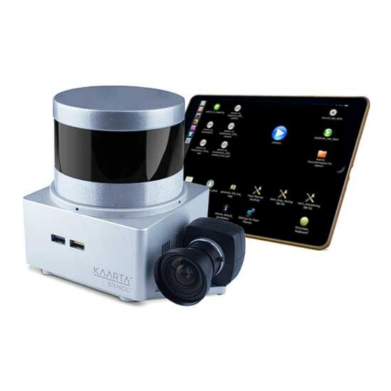
3. Stencil 2 with Tripod Mounting Plate 4. Feature Tracker 5. Velodyne Lidar Sensor, including documentation on the Kaarta USB drive 6. Velodyne Interface Box, AC Supply, and country adapters (not shown) 7. Battery Pack - 23,000 mAH (US shipments only) 8. -
Page 11: Getting To Know Stencil 2 - Older Units
G E T T I N G T O K N O W S T E N C I L 2 - O L D E R U N I T S S/N’s between 100 – 150 [S/N’s between 1 -99 in square brackets] 1. -
Page 12: Status Indicator
S T A T U S I N D I C A T O R Stencil 2 comes with an USB LED Status Indicator. This indicator shows the state of the device and provides alerts in the event of errors. Refer to the table below for definitions of indicator color and states. -
Page 13: Power/Operating Mode Buttons
The USB indicator will illuminate blue when Stencil has completely booted up. After power to Stencil 2 is on and Lidar is on for at least 60 seconds, press the left button once to Start Mapping/Localization. Press again to Stop when mapping/localization is complete. Wait for the yellow USB indicator to stop blinking and turn blue. -
Page 14: Using Stencil 2 Out Of The Box
Turn on Stencil 2, and the Lidar. You’ll know they are on if the LED status ring around each push button and the USB indicator is blue. -
Page 15: Scan Folder Contents
“_replay” added to the folder name when using Stencil 2’s Adaptive Data Replay tool. If you use the upgrade script to convert old Stencil files to the new Stencil 2 format, the subfolder will have “_upgraded” added to the folder name. These subfolders may contain the following files where xxx is the system time when the file was created. - Page 16 Copy these files from Stencil 2 using a USB3 drive with a monitor and mouse. Stencil 2 supports exFAT drives for transferring files larger than 4.3GB. Using USB3 drives reduces the time for data transfers. Be sure to copy data off of Stencil periodically to ensure disk space for future scans.
- Page 17 Open the point cloud, trajectory, and gps data files using CloudCompare software, either on Stencil 2 or on your desktop/laptop computer. Use the Eye Dome Lighting (EDL) function to provide shading so the point cloud is easier to view. In CloudCompare, save the point cloud files in other formats, such as .las. This is helpful for some workflows using CAD software.
-
Page 18: Chapter 2
When processing data in the office, Stencil 2 conveniently works with a computer monitor, keyboard, and mouse. But this set up is not practical for in-field use so Stencil 2 comes with an iPad for changing operating modes, and starting / stopping scans. - Page 19 You should now see the Stencil 2 Desktop on the iPad. The grey menu bar at the top of the screen brings up iPad options in RealVNC. Select the i icon to open the options window. Choose between touchscreen interface or mouse interface.
-
Page 20: Desktop Icons
D E S K T O P I C O N S In addition to the back-panel buttons, Stencil 2 has Desktop icons that control the modes as well as providing a user interface to the many Stencil 2 features. - Page 21 R E C O R D I M A G E S / P L A Y B A C K R A W D A T A Located to the right of the Stencil Start/Stop button are the Playback Raw Data and Record Images Icons.
-
Page 22: Tool Icons
T O O L I C O N S T O O L I C O N S Prepare Upload Stencil 2 will have the ability to upload data to Kaarta Cloud for users to do Replay and other Post Processing operations without the processing and memory limitations of Stencil. - Page 23 Settings for Floor Planner. It will not correct poor maps if Stencil 2 is used for smaller indoor spaces. Loop Closure Correct global drift errors using GNSS and/or trajectory paths that come near each other.
-
Page 24: Mapping With The Feature Tracker
M A P P I N G W I T H T H E F E A T U R E T R A C K E R Stencil 2 is preset to mapping mode without Feature Tracking prior to shipping. Depending on your specific application, mapping without Feature Tracker sometimes produces the best maps. -
Page 25: Feature Tracker Best Practice
Open fields are an example of an extremely sparse 3D structure environment. This is another case where the Feature Tracker should be used to get the best map results. F E A T U R E T R A C K E R B E S T P R A C T I C E For optimal results using the Adaptive Data Replay, you can do live scanning in the three with camera modes. -
Page 26: Recording Color Images While Mapping
R E C O R D I N G C O L O R I M A G E S W H I L E M A P P I N G Stencil 2 saves 1.3 Megapixel color images from the camera. Saving color images cannot be done while using one of the three Feature Tracking (with Camera) modes. - Page 27 Stencil 2 ships with the ability to create detailed maps and provides 6 DoF real time odometry (x, y, z, roll, pitch, and yaw) at 200 Hz with less than 15 msec latency.
-
Page 28: Kaarta User Interface
K A A R T A U S E R I N T E R F A C E The Kaarta User Interface replaces the previous RVIZ window that appears during mapping and localization. There is a parameter in the settings file that can be set to revert to the RVIZ display... - Page 29 Window switcher Window Manager Stop Button Image / Feature Points Pointcloud View / Zoom Disk Space Status Bar Settings The window manager switches the interface between showing two windows (Image / Feature Points and the Point cloud) and one window showing one or the other. The window switcher swaps the larger view (currently with the point cloud in it) with the smaller view (currently with feature points in it).
- Page 30 The leftmost shows an overhead view where you can only rotate the point cloud. Clicking on it will show an isometric view where you can rotate along any axis. The magnifying glass switches between various zoom levels so you can zoom in or see the full extent of the point cloud or something in between.
- Page 31 Here are a couple of the variations described:...
-
Page 32: File Structure-Mapping/Localizing Scans
.bag file, or when converting old Stencil files to the new Stencil 2 format. The top-level scan folder names can be changed to make it easier to recognize and organize scanning files. An example of the top-... - Page 33 Summary scan information can be found in the scan_info.txt file as shown below. Note that the lines indicating GPS Stats only appear in the file if GNSS data was available while mapping or localizing.
-
Page 34: Localization
There are situations where you may wish to generate maps from multiple scans. This is done by first creating a baseline map that Stencil 2 uses as a reference map while collecting more detailed maps, extending maps, or building maps of more complex environments. -
Page 35: Localizing Based On A Prior Map Overview
If you post-processed a map to use, browse and select it or any other map needed. If you choose to use a .ply formatted map not created by Stencil 2, put it in a subfolder in the Recordings directory on the desktop. -
Page 36: Confidence Values
The blue line in the Mapping Plot window is the value of the active confidenceThreshold parameter (default is 0). The localization confidence values are only published by Stencil 2 in live scanning and replay and are not used recorded or used by any of the post-processing tools. - Page 37 See flow chart below for additional insight on mapping and localizing with Stencil 2.
-
Page 38: Chapter 3
T O O L S F O R A D D I T I O N A L F U N C T I O N A L I T Y There are additional tools to help improve both Stencil 2 performance and final point clouds. -
Page 39: Floor Planner Tool
F L O O R P L A N N E R T O O L The Floor Planner tool will auto level, rotate, and generate 2D images of sections from a point cloud file. The tool uses a parameter file accessed through the desktop icon labeled Settings for Floor Planner. - Page 40 Floor Z Search Max (m) - Section of the point cloud to search for the floor plane – The height of Stencil 2 at the start of mapping has an elevation value of zero. If Stencil 2 is set at 2 meters, a value of -0.5 limits the search space for the floor to all z values less than 1.5.
- Page 41 Mean K - the number of points to use for mean distance estimation STD Dev (m) - the standard deviation to use for the maximum distance for keeping the point. Setting this parameter to 2: uses a Radius Outlier Removal Filter (Radius Outlier Removal Filter) where you can specify Clean Radius (m) the radius to look for neighboring points Clean Min K - the minimum number of neighbors in radius to keep the point.
-
Page 42: Command Line Tools
C O M M A N D L I N E T O O L S Kaarta has added a lot of command line scripts to help make post-processing of files easier for the user. Several of these tools can significantly increase the size of the point cloud files as well as delete scalars if run out of order. - Page 43 To select the master scan click on the arrow to the right of the browser and select “Other”. This will open the normal browser panel so you can select the master folder. For the related scans, click on the folder to the right and select all of the folders you want to align. After clicking OK, you should see another dialog box that allows you to select any combination of point clouds, trajectories, gps, and custom files to apply the offsets to.
- Page 44 Update older 2018 files to S20.02 format – This utility will convert scan folders generated prior to the S19.07 Stencil 2 software release. This is critical for generating the scan_info.yaml file needed for Loop Closure using GNSS data and to use Localization using GNSS. It also converts the point cloud to binary which significantly speeds up processing times.
- Page 45 Both of these approaches caused issues when working with 3 party software. Kaarta moved these key times and position offsets (from GNSS) to a machine readable .yaml file so these values could be shared between the operating modes of Stencil, features, and the post-processing tools like loop closure.
- Page 46 Add scalar fields to point clouds – This utility provides an easy way to add additional scalar fields to Kaarta pointcloud.ply files for use in visualization and filtering to produce cleaner and sharper point clouds. The results from live scan and Adaptive Data Replay include x, y, z data with time and intensity.
- Page 47 Normal Calculation Search Distance (m) – This is the radius around a point to include when calculating the normals for that point. Calculate Kaarta Cleaning? – When selected, four additional scalars (KF_1, KF_2, and KF_3) are added to the pointcloud.ply file for use by the movingObjectFilter and pointcloudFilter command line tools.
- Page 48 rosrun pointcloud_cleaning pointcloudFilter _pointcloud_in:= [input filename] _pointcloud_out:=[output filename] _filterBy _kaartaFilter1:=true _kaartaFilter1Threshold:=[value] Filter name Filter variable defaults Units kaartaFilter1 kaartaFilter1Threshold meters kaartaFilter2 kaartaFilter2Threshold none kaartaFilter3 kaartaFilter3Threshold none Scripting support Get the value of a key in a scan_info.yaml file or during a scan – This script which can be embedded in script files will get a value of a key in the .yaml files.
-
Page 49: Cloudcompare Command Line Editor Tool (Alpha Version)
C L O U D C O M P A R E C O M M A N D L I N E E D I T O R T O O L ( A L P H A V E R S I O N ) The CloudCompare Command Line Editor or CC Command Builder (CCCBuilder) Tool is started by typing CCCBuilder in a console terminal. -
Page 50: Using Point Clouds From Other Programs
CloudCompare, it will show the 0, 0, 0 location at the center. Take note of the direction of the X axis (0 radians on the circle) as you will need to point Stencil 2 in the same direction. - Page 51 To adjust the starting location when mapping to a different portion of the map, translate and rotate the point cloud (not the radian circle) in CloudCompare to align it to the Circle_Centered.obj. Be sure the record the 4 X 4 translation matrix to be used to reset the location of the new point cloud collected during localization to the original coordinate system.
-
Page 52: Chapter 4
If the antenna is small enough, it can be mounted to the top of Stencil 2 using double sided tape, etc. If it is larger, you may need to build a suitable frame for mounting the larger antenna such as shown. -
Page 53: Gnss Monitor Status
GNSS Monitor Icon and enter it in the dialogue box. Note: Some GNSS units only work over RS232, which may not register immediately on Stencil 2. To verify that the USB-Serial adapter port is found, type lsusb in a terminal window. If you are still not sure if it is there, remove the GNSS connector and type lsusb again to see if one of the devices is removed. -
Page 54: Recording Gnss Raw Data To Use For Ppk Processing
The black box on the right shows a specific integration using a Trimble BX-992 GNSS unit. Please see the Kaarta Partner Portal for the full Integration Guide (IG-STN-001-0120) showing all the steps for integrating Stencil with the Trimble BX-992 GNSS System. -
Page 55: Using The Loop Closure Tool Overview
rosrun receive_gps binex2GPS_local.sh <.ubx file from the rover> <base unit.obs file> <base unit.nav file> <PLY output file> Note that the <PLY output file> should include the .ply extension. You can now use the corrected gps.ply output in the U S I N G T H E L O O P C L O S U R E T O O L O V E R V I E W The Loop Closure Tool performs global smoothing by introducing loop closure techniques as well as using GNSS inputs for absolute references in correcting drift errors common in mobile mapping systems. -
Page 56: Key Poses And Geo-Locating Point Clouds
The original point cloud, trajectory and GPS files are not modified, but a new sub-folder is added to the current directory with files that have the same timestamp with the “_loop_closed” appended to the name. The gps_20XX-YYY_loop_closed.ply file will contain the points picked for reference when running the Loop Closure Tool with the specific parameters set by the user. - Page 57 589482.266031 4478840.761880 269.389000 589492.266031 4478840.761880 269.389000 589482.266031 4478850.761880 269.389000 589482.266031 4478840.761880 279.389000 589492.266031 4478840.761880 279.389000 589482.266031 4478850.761880 279.389000 Load the text file into CloudCompare as a point cloud. Once you have identified the physical features in the point cloud that correspond with the GCPs in the text file, use CloudCompare to align them as described here: 1.
- Page 58 Be sure the GCPs are labeled as the Reference. 3. Start picking the corresponding points in each cloud. When you have the corresponding pairs selected, you can see the effect of scaling on the error terms and choose to add scaling to the geo-location process. As a rule, do not scale as it distorts the finished cloud to match the points more closely.
-
Page 59: Loop Closure Using Confidence Values
L O O P C L O S U R E U S I N G C O N F I D E N C E V A L U E S Occasionally Stencil generates laser scan matches that are less than optimum. There are two ways to fix this. -
Page 60: Loop Closure With Gnss Data
Another reason to run the data twice is to make use of the confidence values (see previous section) to generate a more accurate trajectory by removing a twist in path before aligning it with the GNSS data. L O O P C L O S U R E W I T H G N S S D A T A Stencil records a GPS_20yy-mm-dd-hh-mm-ss.ply file whenever a GNSS device is attached (and integrated). - Page 61 The files are auto-populated from the latest scan folder. In this example, there was no GPS file, so it is left blank. If you click on the Change Directory button, you can select a different sub-folder to use, if it is not from the latest scan. It should auto-populate the files from that sub-folder. If you want to choose another point cloud, trajectory or GPS file from that sub-folder, you can use the file browser button next to the file names.
- Page 62 Enabled? Checkbox – Uncheck this box if you only want to do GNSS based loop closure and do not want Stencil to do scan matching where trajectories approach each other. Matching Threshold (5000) – Minimum threshold to accept scan matches during the process of aligning the two patches from each part of the trajectory that comes close to each other.
- Page 63 stopping locations of the scan to optimize the places where the Loop Closure Tool will look for potential matches. Match Region Horizontal (15.0 m) – This is the horizontal radius (H) in meters of the two patches to be used for matching where the two trajectories come close enough to each other as identified by match region.
- Page 64 Replay. Setting the number as low as 1 will add significant time to the processing for larger datasets, but may be acceptable when dealing with troublesome spots in the dataset. Pose Stack Confidence Cutoff Value (0.0) – If you set the confidence cutoff in percentile and you set this value at 1.0, the Loop Closure Tool will reject the lowest 1 % of the confidence values over the course of the scan.
- Page 65 GNSS Weight Factor - If the weighting factors are set to 0.0, the point cloud and trajectory files will be translated and rotated into the global coordinate frame without performing any loop closure or geo-registration processes. This means the locally consistent point cloud originally produced by Stencil will not be modified except for rotation and translation into the global coordinate frame.
- Page 66 It is less suitable for longer linear type scans. The Displacement Method tracks the current location from the origin of the scan and calculates the best match between the Stencil 2 and the GNSS trajectories.
- Page 67 Laser or Camera coordinate system manually. Stencil uses the offsets in the parameter file to correctly align the data from the GNSS and the Stencil 2 trajectory. In Mapping / Localization without the feature tracker the trajectory is relative to the mid-point of the lidar.
- Page 68 Pitch Correction Factor – This is the most useful of the four parameters for correcting vertical drift for longer traversals over roads where there are no loops. A typical value to start with is 0.001 radians. This term can be negative if needed. Sometimes this can be useful when the scanner is tilted (resulting in higher drift errors in the z direction) when there is no GNSS data Yaw Correction Factor –...
-
Page 69: Gnss Loop Closure Example
GNSS data showing dropouts over the course of the data collection. The picture at the bottom is the trajectory data from Stencil 2. The starting and ending locations were the same. As you can see there were some issues with Stencil 2 trajectory as the trajectory end points do not match. -
Page 70: Loop Closure Tool Effect
Here is the corrected trajectory in yellow overlaid on the original GNSS data. L O O P C L O S U R E T O O L E F F E C T The next two images show the effect of the loop closure tool. The first image is an intersection that the vehicle passed through three times before correction. - Page 71 The second image shows the same intersection after loop closure was applied. Note that all three passes through the intersection are correctly registered. This last image is the point cloud file overlaid on the a map from maps.google...
-
Page 72: Using Separately Logged Data In The Loop Closure Tool
GNSS data that can fit this model is data from a tracking theodolite that was recorded while mapping with a reflector on top of Stencil 2. To use GNSS data logged separately or non-GNSS data, the data will need to be formatted to fit the Stencil gps_202X-xxx.ply format. -
Page 73: Using Non-Gnss Data For Loop Closure
Aligning the X, Y, and Z positions of the prism to the X, Y, and Z positions of Stencil 2 is done using the loop closure tool similarly to what is described in the section above on using separately recorded GNSS data. -
Page 74: Chapter 5
When mapping over long distances, global smoothing using loop closure techniques can fix double registrations in maps caused by drift. This can be seen sometimes be seen when Stencil 2 sees the same 3D structure at different times in a single scan. This could be caused by enough drift occurring between the sightings that Stencil 2 did not fix the issue through implicit loop closure (for errors less than ¼... - Page 75 use the combined XY and Z distances when computing the 3D Match distance. You can decrease the default horizontal region to 7.5 or less if errors are 2 – 3 meters. You can also decrease the Vertical region 5 if the elevation error is 1 – 2 meters. These numbers represent patches that will be used to match against each time you were in the same area.
-
Page 76: Case Study 2: Ground Vehicle Navigation
1m) and occluding the Lidar field of view as little as possible. If you are indoors in a constrained environment, you can tilt Stencil 2 up to 15 degrees, but if there are bright lights overhead, be sure to point the camera towards the ground (forward or backward) Choose a mapping mode (can be with camera or without) and build a prior map by driving •... -
Page 77: Case Study 3: Air-Ground Collaborative Mapping
Choose a mapping mode, (use with Camera if needed.) Build a ground-based map by hand- • holding Stencil 2 or mounting it to a ground vehicle and moving around the structure. Verify the map has no drift. Run Loop Closure if needed. - Page 78 Note: If the environment has little 3D structure, set useMatching to false (important) during aerial localization (not necessary for ground-based mapping).
-
Page 79: Chapter 6
T I P S F O R C O L L E C T I N G B E T T E R D A T A G E N E R A L If you are doing a lot of indoor scanning in tight spaces and small rooms, consider the Kaarta Contour product. Stencil 2 is meant for larger indoor spaces and outdoor environments. -
Page 80: Handheld Scanning - Indoors
At the start of mapping, wait for points to show up on the monitor or status light to be blinking green, then rotate Stencil 2 slowly while rolling and pitching slightly before moving around to build a denser base map to start from. -
Page 81: Vehicle Mounted Scanning
While tilting the scanner at angles greater than 45 degrees, ensure there is structure in front of and behind the scanner and that the feature tracker is pointed towards the ground and not the sky. For scanning higher up on buildings or trees, first build a solid base map with Stencil horizontal and then tilt and repeat the base scan, once at about 30 degrees, then 60. -
Page 82: Aerial Scanning
R E Q U E S T F O R A D D I T I O N A L S C A N N I N G T I P S Please submit any additional tips to info@kaarta.com for possible inclusion in future revisions of... -
Page 83: Problems / Issues
. P L Y F I L E E R R O R O R N O N - G E N E R A T I O N If Stencil 2 is accidently turned off while scanning or saving the point cloud at the end of a data collection, it may be recovered by using the tools described in the Post-processing Command Line Tools section of this manual. -
Page 84: Double Registration
An uncompensated twist in the trajectory due to lack of 3D structure in the scene Excessive, dynamic motions To address issue 1, Stencil 2 comes with a loop closure tool. The images below show the same data set before (left) and after (right.) Issue 2 is corrected by cutting the point cloud at the twist and remerging the two clouds correctly. -
Page 85: Small Rooms/Narrow Hallways
S M A L L R O O M S / N A R R O W H A L L W A Y S The limited vertical field of view of the Velodyne 16 and 32-line 3D lidars work very well in outdoor and large indoor spaces. -
Page 86: Reflections
F-Stop on the feature tracker to let in more light or limit the amount of light through the lens. Normally it is set to F-4. Stencil 2 uses an auto-exposure algorithm to maximize the dynamic range, but in environments outside the normal limits of darkness/brightness, you can... -
Page 87: Using Cloudcompare
(http://www.danielgm.net/cc/) is an open source software application written for the Mac, PC, and Linux. It is released under the GNU General Public License (GPL). Kaarta uses CloudCompare extensively to view and edit point clouds generated by Stencil and Contour products as well as uploads received and processed by our SaaS Website at uploads.kaarta.com. - Page 88 Typically, start with the Eye Dome Lighting (EDL) shader. It is very fast and outlines edges that make it easier to visualize point clouds. Alternatively, use PCV shading for other interesting effects. After selecting the point cloud to be shaded in the DB Tree toolbox on the left side, select Plugins > P.C.V. (Ambient Occlusion) from the top menu bar to create lighting/shadow effects.
-
Page 89: Colorize Point Cloud By Z-Coordinates
C O L O R I Z E P O I N T C L O U D B Y Z - C O O R D I N A T E S If you want to colorize the point cloud based on Z-coordinates (elevation), select edit>colors>height ramp from the top menu bar. -
Page 90: Colorizing The Point Cloud By Time Using Scalar Fields
C O L O R I Z I N G T H E P O I N T C L O U D B Y T I M E U S I N G S C A L A R F I E L D S The trajectory.ply file contains all 6 DOF values of x, y, z, roll, pitch, and yaw. -
Page 91: Colorization Scales And Intensity Values
C O L O R I Z A T I O N S C A L E S A N D I N T E N S I T Y V A L U E S Velodyne lidars record intensity values and are frequently included in point cloud data. When loading point clouds, it is best to load the intensity values as a scalar value to apply unique colorization scales to the values. - Page 92 As you can see, the lane markings, crosswalks and turn arrows are illuminated. You can further highlight these by changing the color scale associated with this scalar. To do this, select the point cloud in the left side of the DB Tree section, then select the settings gear on the right side of the Color Scale Current selection in the Parameters section.
- Page 93 You can now set a custom colorization to highlight the intensity values. Start by clicking in the middle of the grey color bar. A new crayon tip will appear. If you select the Color box below, you can set this to yellow. Clicking the crayon tip on the right will bring up the white Color box.
-
Page 94: Geo-Locating Point Clouds
G E O - L O C A T I N G P O I N T C L O U D S If you have survey GNSS data such as Ground Control Points (GCP) but no trajectory or time estimates, you can still geo-locate / geo-reference your point cloud using CloudCompare, even though you cannot geo-register your data with the Loop Closure Tool. - Page 95 15. Select both point clouds in the left menu box then use the Align (point pairs picking) tool under the Registration submenu to associate the GCP with the corresponding point in the point cloud. 16. Be sure the GCPs are labeled as the Reference. 17.
-
Page 96: Cleaning And Merging .Ply Files
C L E A N I N G A N D M E R G I N G . P L Y F I L E S : P O I N T C L O U D C L E A N U P 1. -
Page 97: Merging Point Clouds
20. Save both point clouds in case you run into issues in the next step and need to start over. M E R G I N G P O I N T C L O U D S 21. Load the .ply files you want to merge into CloudCompare. 22. - Page 98 Step 1: Downsize point clouds before ICP matching. Load both the ground map (gray) and aerial map (green). Manually move the aerial map toward the ground map. Bring both point clouds close to each other. As you see in the figure, the aerial map is still misaligned with the ground map a bit.
- Page 99 Step 3: Repeat ICP matching multiple times to make sure of convergence. Once you have subsampled and segmented map you want to transform, you can drag the original point cloud under it so that the transformation calculated on the subsampled and segmented map is also applied to the full map.
- Page 100 You may need to give the ICP matching multiple tries. Observe the example below where it was run twice. As in the figures, the transformation matrix shows some higher values on the last column after the first try. After the second try, the values become very small, indicating good coverage matching.
- Page 101 If you did not move the full-size aerial point cloud under the subsampled one, you will need to apply the transforms generated by the ICP process in the order they were done. Do not use the values from the Register info box as they are truncated. The console window under the point cloud will have the transformations.
-
Page 102: Chapter 7
F A Q My robot drives in flat areas, how can I estimate planar motion instead of 6-DOF motion? Mount Stencil 2 horizontally on the robot. Using the Stencil Settings icon, update the usePlanarMotion to true in the user parameters. - Page 103 How do I update the map for localization after changes in the environment? Conduct a localization scan using Stencil 2 based on your prior map. You can either merge the two maps and save the file or just use the new map created. Run the Choose Map for Localization to replace the map by the newly generated map.
- Page 104 Velodyne with respect to Stencil 2. Also, to ensure synchronization, be sure to use the same wiring as the cable supplied by Kaarta to connect the Velodyne to Stencil 2. Kaarta sells a version of Stencil / Traak with an external IP65 rated IMU.
- Page 105 • What version of Software am I running on Stencil 2? Stencil 2 runs Ubuntu 16.04. IMPORTANT: Do not update Ubuntu or the ROS packages on your Stencil 2 as it will break the mapping system. All Stencils shipped prior to July 2018 are running Ubuntu 14.04 unless their software has been updated.
- Page 106 See the following link for more information. (http://www.gpsinformation.org/dale/nmea.htm#nmea). The three common message types supported by Stencil 2 where XX can be GP, GL, GN, BD, etc., contains the essential 3D location, time, and accuracy data. As an example, one $XXGGA message protocol is shown here: $XXGGA –...
- Page 107 The loop closure tool works with any number of GNSS points if the timestamp associated with the GNSS point matches the right point in the Stencil 2 trajectory. If you set the data rate to 5 Hz, Stencil 2 saves a GPS point for every trajectory point. But even 5 or 10 GNSS points spread out over the entire data collection will be enough to significantly reduce global drift.
-
Page 108: Customizing Velodyne Wiring
Please contact Velodyne or Kaarta for more details. Customers who choose to assume the cost of non-warranty repairs can modify their Velodyne cable to connect to Stencil 2. Kaarta will not warrant customer-made cabling that causes damage to Stencil 2 or the lidar. - Page 109 Velodyne is on the same side as the button side of Stencil. See the photograph below for the correct orientation. Note: You must use the Velodyne in the factory default configuration with Stencil 2 with the following except as noted in item 5 above. +12VDC...
-
Page 110: Mounting Stencil 2
M O U N T I N G S T E N C I L 2 Stencil 2 ships with a tripod adapter plate for ease of mounting with handheld or vehicular applications. This plate uses the world-wide standard ¼-20 tripod mounting thread. -
Page 111: Parameter Definitions
A P P E N D I X I I I P A R A M E T E R D E F I N I T I O N S Changing parameters currently uses the Atom text editor to make changes. The editing window is split into three parts. - Page 112 – If set to false, the user will have to manually start the visualization • window for scanning. type: kaarta_ui - use the Kaarta UI for visualization during live scanning and replay. • Change to “rviz” to revert to the classic older Stencil RVIZ visualization kaarta_ui_rviz_config_dir: /home/stencil/install/share/ros_ui/rviz/ - directory for the •...
- Page 113 – This parameter will delete a gps file after scanning if • the file was created but contains no data. sensorOffsets: Offsets between the GNSS unit and the lidar on Stencil 2. The ones listed here are for the Emlid Reach+ as mounted using Kaarta’s GNSS mounting bracket. •...
- Page 114 velodyneCloudGenerator: maxPointNum: 30000000 - Maximum number of points in the preview point cloud. For • longer scans like an hour, increase this number to 90000000. The purpose of the preview cloud is to quickly look at results in the field. A smaller cloud for post-processing also helps if you need to make multiple tries to find the right parameters for the Loop Closure Tool.
- Page 115 • reduce the values by 50 %. In open areas, increase by 50 %. surroundVoxelSize: - Resolution of the point cloud for display in the Kaarta UI (or RVIZ). • localizationDecayDis: 25 – Decay distance used in localization modes to ensure you •...
- Page 116 and paths that intersect frequently. Setting a value of 35 - 65 is useful for longer linear scans where you do not come back to an intersecting trajectory frequently. This parameter is useful to prevent incoming scan data from being registered against a part of the registered map that has drifted over longer distances distorting the map locally which cannot be fixed using the Loop Closure Tool.
- Page 117 eigenvalueThreshold: 100 - Threshold for evaluating degeneracy - Can change based • on scenario, i.e. outdoor vs indoor scan. maximumIterations: 10 – Max number of iterations to use for matching scan frames. • Increase to 25 or 50 only for playback as it greatly increases processing load for real time scanning.
- Page 118 10 – Size in GBytes to stop/prevent scanning to preserve. • receive_xsens: imu_port: /dev/ttyUSB0 - Configured at the factory. Not meant for user changes • use_chrony: false - Set to true if synchronizing a customer computer to Stencil 2. •...
- Page 119 – additional IMU data available from the driver • cloud_nodelet: upward: true - set to false if mounting Stencil 2 upside down, at the same time set • laser_wrt_imu_roll (under receive_xsens on the next line) to 3.1415926. Do not need to do this in mapping / localization with camera modes.
- Page 120 Kaarta Cloud Settings kaarta_cloud: auto_create_zip: false – If set to true, a zip file will be created at the end of each scan or • replay for uploading to Kaarta Cloud.
- Page 121 Replay Settings playback: override_rate: -1 If this number is <= 0, use Adaptive Data Replay. If this number is > 0, • use the value as the fixed replay rate. i.e. 0.5 would be to replay the data at half speed, etc. pause_at: [ ] - Comma separated list of times in the replay that you would like the replay •...
-
Page 122: Typical Parameters To Set
T Y P I C A L P A R A M E T E R S T O S E T S T R U C T U R E D O U T D O O R / L A R G E I N D O O R E N V I R O N M E N T S In structured outdoor or large indoor environments, use the default values: voxelSize: 0.2 surfVoxelSize: 0.4... - Page 123 T I G H T I N D O O R E N V I R O N M E N T S Environments such as office spaces and underground mines, you can do really well when using the Adaptive Replay Tool.
-
Page 124: Working With Ros
These commands are the same as the big blue Play button on the Stencil 2 desktop. You should open two ssh terminals on the remote desktop. One for switching the mode and issuing stencil_start, the second one to issue stencil_stop. If you Ctrl-C in the start window, it doesn't do all of the shutdown steps like generating the preview map or organizing files. -
Page 125: Remote Commands Not Supported
R E M O T E C O M M A N D S N O T S U P P O R T E D Stencil 2 does not support any of the tools or playback from a remote terminal at this point. This includes sharpening, floor planner, loop closure or playback of raw data files. -
Page 126: Important Localization Topics
R E P O R T I N G G L O B A L P O S I T I O N D U R I N G L O C A L I Z A T I O N Stencil 2 can localize on a geo-referenced map created by Stencil 2 using the Loop Closure tool with GNSS data. - Page 127 3) You will need to have a fix quality of 4 (preferred) or 5 (might work) when you start the Localize using GNSS tool. If your GNSS position estimate is not accurate enough, you may not be able to lock onto the correct position. It should be within 0.5 meters of the correct position.
-
Page 128: Sensor Calibration
These define relative orientation of the Velodyne with respect to the IMU. Translation between the two sensors is not used. If mounting Stencil 2 underneath the Velodyne, the sensors are physically aligned. The three angles are zeroes for the shipped configuration. - Page 129 This is the data saved in the trajectory.ply file. /aft_mapped_to_map Same as above, but in the map origin frame /autoExp /clicked_point Returns position of mouseclick in rviz window /clip_mode Kaarta UI ceiling clipping: not implemented /cmd_back, /command Kaarta UI: not implemented /continue_adr /diagnostics /fused_data_latest_pose, /fused_data_output, /fuser_reset /geo/global_pose,...
- Page 130 ROS topics while mapping Additional ROS topics Description while localizing origin of the map of the localization run. If you start at the origin, it should be the same as integrated_to_init /isSensorMoving Should be set to false to freeze the current pose. Useful when robot is stopped in location where there is significant occlusions or larger moving objects in the environment.
- Page 131 ROS topics while mapping Additional ROS topics Description while localizing /monocular_camera/image/theora, /parameter_descriptions, /parameter_updates /monocular_camera_highres/change_rb_gain, Kaarta UI: not implemented /monocular_camera_highres/exposure_lock, /monocular_camera_highres/gain_setting /move_base_simple/goal /os1_node/imu_packets, Data from the OS-1 sensor. Works in replay mode only. /os1_node/lidar_packets /pose_reset You can publish a pose on this topic and the localization estimate will jump to that position.
- Page 132 ROS topics while mapping Additional ROS topics Description while localizing /tf, /tf_static /throttle_registration /tobe_mapped_to_init /total_point_num /ueye_cam_nodelet/parameter_descriptions, /parameter_updates /ueye_cam_nodelet_manager/bond /velodyne_cloud_from_registration_full_res /velodyne_cloud_mapped The latest velodyne point cloud after being registered to the map frame /velodyne_cloud_registered Final point cloud output. The latest velodyne point cloud after being registered to the init frame /velodyne_gps_fix /velodyne_nodelet_manager/bond...
-
Page 133: Replaying Stencil 2 Data
R E P L A Y I N G S T E N C I L 2 D A T A Stencil 2 can replay raw data (.bag files) with different parameters if a raw data (.bag) file was saved during the real time processing. This option is enabled at shipment. - Page 134 Users can customize Stencil 2 parameters by double clicking the desktop icon for Stencil Settings. This will bring up a text editor with three sections. The section on the right side are the Stencil 2 default parameters. Users can modify these default parameters by copying them over from the default side (right side of the screen) over to the user defined parameters (left side) and modifying the left side to the desired values.
-
Page 135: Replaying Bag Files In Localization Mode
Localization is a powerful feature for registering point clouds together without having to go through a separate alignment process. Localization ensures point clouds from Kaarta’s mobile mapping system can be joined seamlessly. It is pretty straightforward to replay a file in localization mode that was already collected in either mapping or localization mode. - Page 136 Circle_Centered.obj moved to .raw data file origin Circle_Centered.obj 3. Use the point picking tool to select the new origin point and record the X and Y values. Remember to adjust the Z value for the expected height of Stencil above this point.
- Page 137 4. Create the XXX_pose.txt with the X, Y, and yaw values recorded. Remember to enter the yaw value in radians. In this example, the file would look like this: # [2020-02-07 17:41:02 EST] # Last pose format: xyzypr 29.38 4.31 0.0 1.6 0.0 0.0 5.
- Page 138 Stencil 2 is synchronized internally between the Velodyne, IMU, and computer. It is also possible to synchronize a Linux based computer that is running ROS to Stencil 2. This allows it to share localization and point cloud data in real time.
- Page 139 ROS_MASTER_URI=http://Stencil:11311. Save and Close the file. Run source ~/.bashrc to apply to the current terminal window. To verify it is working, open a terminal window on Stencil 2 and run roscore. While the core is still running open a new terminal window and type rosrun rospy_tutorials talker.py. It should start printing out Hello World with time stamps.
- Page 140 RVIZ on the Customer Computer with the Stencil 2 RVIZ configuration. To do this, first find the Stencil 2 RVIZ configuration file (clay_cam_v16.rviz if using a VLP-16 or clay_cam_v32.rviz if using an HDL-32) copy it onto the Customer Computer. It is located in ~/stencil/install/share.
- Page 141 Internet, rather than Stencil 2. Please make sure Stencil 2 is the only timeserver. Note: If the Stencil 2 IP address was modified to something other than 10.1.1.100, open the chrony configuration file (in a terminal window run sudo gedit /etc/chrony/chrony.conf) and change the line server 10.1.1.100 minpoll 1 maxpoll 2 in the file correspondingly.
- Page 142 If for any reason, the power is removed from Stencil 2 before the save operation has completed, you may still be able to recover the map by using the Post Processing Command Line Tools to repair the incomplete files.
- Page 143 GNSS Tighter GNSS Simplified instructions for integrating GNSS devices with integration Stencil 2. Stencil 2 records GNSS data for use in loop closure to geo-register datasets. Easier localization Localization map and last pose pointers provide more intuitive operation when conducting multiple localization mapping scans.
- Page 144 2 current with Kaarta Contour ® Software Improved Stencil 2 now reads and writes the file headers, so data is read/write not lost when running loop closure or sharpening tools. The updated file format lets you record confidence estimates and prevents CloudCompare from corrupting time values.
- Page 145 A quad core processor improves real-time capabilities processor and reduces overhead issues over the previous dual core New sensors Stencil 2 now works with the VLP-32C and the feature tracker can be used with the 32 line scanners File size Binary point Take up less space than the text-based point cloud files.
- Page 146 N E W F O R S O F T W A R E R E L E A S E S 1 9 . 0 7 ( J U L Y 2 0 1 9 ) New command Scripts have been created to fix most common issues line tools related to power failures, converting older datasets to the new formats, fixing vertex values, ascii/binary...
- Page 147 Movie files Stencil 2 will create time-stamped images and an avi movie file if Record Images is turned on during scanning. Confidence Plot The Confidence plot shows the values for Mapping...
Need help?
Do you have a question about the STENCIL 2 and is the answer not in the manual?
Questions and answers