Page 1 Products: ASC500 User Manual ASC500 SPM Controller & Software v2.5 attocube systems AG, Königinstrasse 11a (Rgb), D - 80539 München Germany Phone: +49 89-2877 80915 Fax: +49 89-2877 80919 E-Mail: info@attocube.com www.attocube.com For technical queries, contact: support@attocube.com attocube systems office Munich:...
Page 2 Page 2...
Page 3: Table Of Contents
Profile configuration ............ 51 Page 3 © 2001-2011 attocube systems AG. Product and company names listed are trademarks or trade names of their respective companies. Any rights not expressly granted herein are reserved. ATTENTION: Specifications and technical data are subject to change without notice.
Page 4 V.3.a. User-configurable GUI appearance ........ 51 V.3.b. Aliases menu ............51 V.3.c. New signal and parameter names in v2.5 ......54 V.4. General Usage and Description of Common GUI Controls ..55 V.4.a. Text Edit Boxes ............55 V.4.b. Context Menu ............56 V.4.c.
Page 5: Introduction
Warning, laser radiation. Do not stare into beam. Class 1M Laser product. Page 5 © 2001-2011 attocube systems AG. Product and company names listed are trademarks or trade names of their respective companies. Any rights not expressly granted herein are reserved. ATTENTION: Specifications and technical...
Page 6: I.2.A. Warnings
There are no user-serviceable parts inside the electronics. Modified or opened electronics cannot be covered by the attocube warranty anymore. Take special care if connecting products from other manufacturers. Follow the General Accident Prevention Rules.
Page 7 5° to 40°C, 20% to 80% RH. Page 7 © 2001-2011 attocube systems AG. Product and company names listed are trademarks or trade names of their respective companies. Any rights not expressly granted herein are reserved. ATTENTION: Specifications and technical...
Page 8: Declarations Of Conformity
Changes or modifications not expressly approved by attocube systems could void the user’s authority to operate the equipment.
Page 9: Waste Electrical And Electronic Equipment (Weee) Directive
Page 9 © 2001-2011 attocube systems AG. Product and company names listed are trademarks or trade names of their respective companies. Any rights not expressly granted herein are reserved. ATTENTION: Specifications and technical data are subject to change without notice.
Page 10: Hardware Description
Hardware Description II.1. Mechanical Installation Siting Unpack all the components and retain all packing material and shipping container for your future shipping needs. When placing the controller, do not obstruct the ventilation slots in any way. Make also sure that the controller is not paced close to any liquids or moisture.
Page 11: Ii.2. Electrical Installation
Always replace broken fuses with a fuse of the same rating and type. Page 11 © 2001-2011 attocube systems AG. Product and company names listed are trademarks or trade names of their respective companies. Any rights not expressly granted herein are reserved. ATTENTION: Specifications and technical...
Page 12: Ii.3. Front And Rear Panel Connections
USB connector for connection to a PC, the serial connector to connect to the ANC150. II.3.c. Cable description ASC500 v1 Power supply: Use the power cable to connect the ASC500 to the 100, 115 or 220 V jack. Page 12...
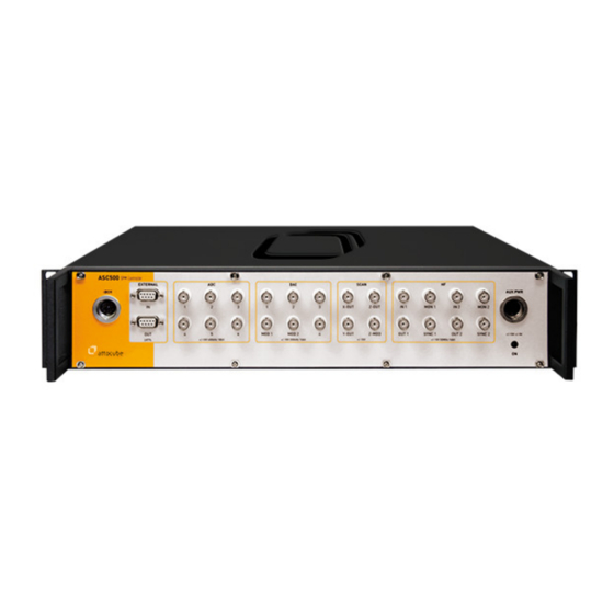
Page 13: Ii.3.D. Front Panel Asc500 V2
The differences between the two Page 13 © 2001-2011 attocube systems AG. Product and company names listed are trademarks or trade names of their respective companies. Any rights not expressly granted herein are reserved. ATTENTION: Specifications and technical...
Page 14 Figure 3: Front panel of the ASC500 v2. The break-out cable of v1 was replaced by easily accessible BNC connectors at the front panel. Please note that both input and output ranges and sampling rate of all converters are indicated directly below the connector plugs.
Page 15: Ii.3.E. Back Panel Asc500 V2
(called NSL A and NSL B) and a LAN connector. Figure 5: Back panel of the ASC500 v2. Please note the new digital interface (NSL) and the LAN connection. The connectors will be described in more detail from left to right: Power connection: Connection to mains.
Page 16: Ii.4. The Ibox
Using the ASC500-iBox, the main scan- and feedback parameters can be accessed manually. This enables e.g. precise and fast control of the feedback loop and the scanning process itself. Figure 6: The ASC500-iBox (bottom) for manual control of all important scan and feedback parameter. Page 16...
Page 17 I.1.a). Page 17 © 2001-2011 attocube systems AG. Product and company names listed are trademarks or trade names of their respective companies. Any rights not expressly granted herein are reserved. ATTENTION: Specifications and technical data are subject to change without notice.
Page 18: Iii. Description Of The Controller
III. Description of the Controller III.1. Key Features and Benefits AFM/SNOM Control 18 bit 400 kS/s ADC input-channel for AFM contact mode signal • digital measurement of frequency and phase for AFM non-contact • mode with feedback DDS for oscillation excitation / frequency range 1 kHz to 2 MHz •...
Page 19: Iii.3. General Functionality
All signals are acquired during both forward and backward motion. Page 19 © 2001-2011 attocube systems AG. Product and company names listed are trademarks or trade names of their respective companies. Any rights not expressly granted herein are reserved. ATTENTION: Specifications and technical...
Page 20: Iii.4. Hardware Requirements And Operating Systems
‘ASC500_Software’) and the drivers (folder ‘ASC500_Driver’) from the CD onto your computer. When the ASC500 is connected to the computer and switched on for the first time, the computer should recognize the new hardware. Please follow the steps below to install the driver.
Page 21: Iii.5.A. Windows Xp
Click “Next” to get to the following window. Page 21 © 2001-2011 attocube systems AG. Product and company names listed are trademarks or trade names of their respective companies. Any rights not expressly granted herein are reserved. ATTENTION: Specifications and technical...
Page 22: Iii.5.B. Windows Vista / Windows 7 (32/64 Bit)
In case a window as shown on the left appears, indicating that the driver has not passed the Windows Logo Test, press “Continue Anyway” to proceed with the installation. Finish the installation. III.5.b. Windows Vista / Windows 7 (32/64 bit) Go to Control Panel ->...
Page 23 …to start the driver installation. Page 23 © 2001-2011 attocube systems AG. Product and company names listed are trademarks or trade names of their respective companies. Any rights not expressly granted herein are reserved. ATTENTION: Specifications and technical data are subject to change without notice.
Page 24 Click Close to finish the installation procedure. Page 24...
Page 25: Data Handling
(GUI) via the icon that is shown to the left. Page 25 © 2001-2011 attocube systems AG. Product and company names listed are trademarks or trade names of their respective companies. Any rights not expressly granted herein are reserved. ATTENTION: Specifications and technical...
Page 26 Figure 8: The Data Channel Configuration dialogue. Figure 8 shows the DCC in one example configuration. There will always be one channel predefined in the LINE and FFT group. Only a filename has to be defined. The AVG checkboxes should be turned ON and both SNAPSH and ASCII should be checked under DISPLAYED.
Page 27 Page 27 © 2001-2011 attocube systems AG. Product and company names listed are trademarks or trade names of their respective companies. Any rights not expressly granted herein are reserved. ATTENTION: Specifications and technical...
Page 28: Iv.1.B. The Snapshot Preset Configuration
display. A snapshot trigger in a SCAN display will save the data of all SCAN data channels simultaneously. The data will be stored in a multitude of formats: for example the SCAN data of Figure 8 will be saved in ASCII and binary type format and in addition as a PNG picture file.
Page 29: Iv.2. Data Handling Details
Data Collection module. Page 29 © 2001-2011 attocube systems AG. Product and company names listed are trademarks or trade names of their respective companies. Any rights not expressly granted herein are reserved. ATTENTION: Specifications and technical...
Page 30: Iv.2.C. Data Processing Chain
IV.2.c. Data processing chain The diagram of the data processing chain is shown in Figure 11. All signals are either recorded or generated within the physical unit of the ASC500 controller. The data is then averaged according to the user’s settings (defined in the DCC, see IV.2.e).
Page 31: Iv.2.D. Sample Time And Average
DCC. It is set to Average ON for all channels per default. Page 31 © 2001-2011 attocube systems AG. Product and company names listed are trademarks or trade names of their respective companies. Any rights not expressly granted herein are reserved. ATTENTION: Specifications and technical...
Page 32: Iv.2.E. Data Channel Configuration (Dcc) In Detail
IV.2.e. Data Channel Configuration (DCC) in detail A central point for the configuration of the data processing chain is the Data Channel Configuration dialogue (DCC). It can be accessed from various points in the graphical user interface by clicking on the DCC button shown to the left.
Page 33: Iv.2.F. Dcc Usage
This number cannot be Page 33 © 2001-2011 attocube systems AG. Product and company names listed are trademarks or trade names of their respective companies. Any rights not expressly granted herein are reserved. ATTENTION: Specifications and technical...
Page 34: Iv.2.G. Saving The Data
edited. 3 – Reset the File No to 0. 4 – Filename used for storing the data of the data channel. 5 – The Signal that will be routed into the data channel. 6 – Average button. The signal will be averaged over its sample time. See IV.2.d for more details.
Page 35 Page 35 © 2001-2011 attocube systems AG. Product and company names listed are trademarks or trade names of their respective companies. Any rights not expressly granted herein are reserved. ATTENTION: Specifications and technical...
Page 36 data. The differences between LINE/FFT compared to other data groups is also highlighted in the splitting of the DCC, where LINE and FFT are shown in an extra lower part of the DCC window. Filename Convention The filename will be composed from several parts. First, there will be a prefix referencing the data group and an index number.
Page 37 5. Page 37 © 2001-2011 attocube systems AG. Product and company names listed are trademarks or trade names of their respective companies. Any rights not expressly granted herein are reserved. ATTENTION: Specifications and technical...
Page 38: Iv.2.H. Parameter File
This format is a picture type format for screen snapshots. It is available for PNG Format all data and display types. The content of the display is saved to hard disk as it is shown on the screen. For SCAN and similar data, there will be always the forward and backward scan direction saved to a separate file (even if only one direction is shown in the display).
Page 39 P0001-ln_1-Line View.csv Page 39 © 2001-2011 attocube systems AG. Product and company names listed are trademarks or trade names of their respective companies. Any rights not expressly granted herein are reserved. ATTENTION: Specifications and technical data are subject to change without notice.
Page 40 This filename is composed as follows: Preset 0 was used to create the file index number data channel name taken from the DCC ln_1 Name of the display (marks that data was saved AS Line View DISPLAYED) text type data format (‘comma separated values’) .csv How to trigger a snapshot preset...
Page 41: Operating The Controller: General Usage And Overview
Page 41 © 2001-2011 attocube systems AG. Product and company names listed are trademarks or trade names of their respective companies. Any rights not expressly granted herein are reserved. ATTENTION: Specifications and technical data are subject to change without notice.
Page 42: V.2. Description Of Main Daisy Program
Also, it can reboot the controller and send new boot code. Yet, for controlling parameters and outputs of the ASC500, a profile has to be loaded that defines the graphical user interface (GUI). A profile (*.ngp) consists of saved settings and a panel (*.ngc).
Page 43 Settings. Page 43 © 2001-2011 attocube systems AG. Product and company names listed are trademarks or trade names of their respective companies. Any rights not expressly granted herein are reserved. ATTENTION: Specifications and technical data are subject to change without notice.
Page 44: V.2.B. The Menu Bar
V.2.b. The menu bar In addition to the standard menu entries as already described above, there are the following options available in the main menu bar: The File menu contains the following entries: Load Profile: Click here to load a profile (.ngp). Load Panel: In addition to profiles (.ngp), there is also a number of preconfigured panels (.ngc) available.
Page 45 Page 45 © 2001-2011 attocube systems AG. Product and company names listed are trademarks or trade names of their respective companies. Any rights not expressly granted herein are reserved. ATTENTION: Specifications and technical data are subject to change without notice.
Page 46 In this tab, you can change the different Feedback Clocks. In this tab, you can change the assignments for some iBox knobs to certain signals: Z Offset: Choose between Z Out and Z Offset. Proportional & Integral: Choose between Z Feedback, Amplitude Feedback and Frequency Feedback.
Page 47 Page 47 © 2001-2011 attocube systems AG. Product and company names listed are trademarks or trade names of their respective companies. Any rights not expressly granted herein are reserved. ATTENTION: Specifications and technical...
Page 48 For a description of this tab, please see section 0 on page 67. Transfer Functions The Transfer Functions offer the following functionalities: 1. Conversion of the voltage values read by ADC inputs towards physical meaningful units. For example, if a photo-detector is used to collect your data, Daisy can display all data in Watts.
Page 49: V.2.C. Loading A Profile
Page 49 © 2001-2011 attocube systems AG. Product and company names listed are trademarks or trade names of their respective companies. Any rights not expressly granted herein are reserved. ATTENTION: Specifications and technical data are subject to change without notice.
Page 50 Special GUIs are available for all attocube systems microscopes. These have been developed to adapt for the use of the specific instrument. In the CFM GUI for example, there are less controls and parameters to facilitate the usage with the confocal microscope.
Page 51: V.3. Profile Configuration
V.3.b. Aliases menu Since both the ASC500 hardware as well as the Daisy software serve the purpose of a very generic, multipurpose and powerful SPM controller, many of the signals, parameters and tab names within the software have also been kept as generic as possible.
Page 52 Simply type in new Aliases for any of the shown Input signal names and click OK. Simply type in new Aliases for any of the shown Output signal names and click OK. Page 52...
Page 53 Page 53 © 2001-2011 attocube systems AG. Product and company names listed are trademarks or trade names of their respective companies. Any rights not expressly granted herein are reserved. ATTENTION: Specifications and technical data are subject to change without notice.
Page 54: V.3.C. New Signal And Parameter Names In V2.5
V.3.c. New signal and parameter names in v2.5 Starting from v2.5, several signals, parameters and tabs in the GUI have been renamed compared to previous versions of the Daisy software (or have been equipped with the opportunity of aliases). The following table lists the changes in order to help existing users with an updated Daisy software to get an overview of the mapping between old and new names: Previous name...
Page 55: V.4. General Usage And Description Of Common Gui Controls
SHIFT and/or STRG key during turning of the mouse wheel. Page 55 © 2001-2011 attocube systems AG. Product and company names listed are trademarks or trade names of their respective companies. Any rights not expressly granted herein are reserved. ATTENTION: Specifications and technical...
Page 56: V.4.B. Context Menu
By right-clicking on any graph window, one can open the corresponding V.4.b. Context Menu context menu. The functions that are available to the graphs are the same throughout the program. The context menu looks as follows: Clicking on ‘Ranges…’ leads to the following dialog: Ranges The X Range and Y Range of the graph can be explicitly set.
Page 57 Daisy window and selecting Attach Window. Page 57 © 2001-2011 attocube systems AG. Product and company names listed are trademarks or trade names of their respective companies. Any rights not expressly granted herein are reserved. ATTENTION: Specifications and technical...
Page 58: V.4.C. Frame View Context Menu
Frame View The Frame view context menu offers mainly the same options as described V.4.c. context above, but in addition, one can also activate a 3 dimensional data view (3D menu view), and/or change the Color Coding. One can choose the colors which provide best contrast for the data.
Page 59 Press Finish. Page 59 © 2001-2011 attocube systems AG. Product and company names listed are trademarks or trade names of their respective companies. Any rights not expressly granted herein are reserved. ATTENTION: Specifications and technical data are subject to change without notice.
Page 60 The new window will appear. Detach it from the Daisy window, or keep it as another tab within your main window. The signal can be chosen via the drop down list in the upper left of the window. Set the Scan Direction Filter according to your needs (forward or backward;...
Page 61 IV.1 for details.) Page 61 © 2001-2011 attocube systems AG. Product and company names listed are trademarks or trade names of their respective companies. Any rights not expressly granted herein are reserved. ATTENTION: Specifications and technical data are subject to change without notice.
Page 62: Description Of The Afm Profile
If in doubt, please contact attocube’s technical support. Caution. The output limit is the voltage supplied by the ASC500 controller. This voltage is then typically fed into a voltage amplifier (e.g. the ANC300) which amplifies this voltage by some factor before it is applied to the piezos.
Page 63 (green) or not (red). Page 63 © 2001-2011 attocube systems AG. Product and company names listed are trademarks or trade names of their respective companies. Any rights not expressly granted herein are reserved. ATTENTION: Specifications and technical data are subject to change without notice.
Page 64: Vi.2. The Scanner Control
VI.2. The Scanner Control The scanner widget is the control center of the scan generation. All important scan parameters, such as the number of Scan Lines and Scan Columns, Pixel Size, and Sample Time can be entered here. Furthermore, an offset for the scan area can be set (Origin X and Origin Y).
Page 65 Dual Pass: Use this option for the Dual Pass mode, see also section VI.5.g. Page 65 © 2001-2011 attocube systems AG. Product and company names listed are trademarks or trade names of their respective companies. Any rights not expressly granted herein are reserved. ATTENTION: Specifications and technical...
Page 66 In this mode, every line is scanned twice (fwd-bkwd, fwd-bkwd, next line). The Scan Display gives an overview over scan range and active scan area. In The Scan Display its smallest magnification, the total available scan range is visible and marked by a red rectangle.
Page 67: Vi.2.A. Closed Loop Scanning
Page 67 © 2001-2011 attocube systems AG. Product and company names listed are trademarks or trade names of their respective companies. Any rights not expressly granted herein are reserved. ATTENTION: Specifications and technical...
Page 68 2. The sensor signal is an analog voltage that has to be fed into the ADC5 input of the ASC500 for the x direction sensor and into the ADC6 input for the y direction sensor. It is not possible to change the input configuration to other ADC inputs.
Page 69 The red dot will NOT Page 69 © 2001-2011 attocube systems AG. Product and company names listed are trademarks or trade names of their respective companies. Any rights not expressly granted herein are reserved. ATTENTION: Specifications and technical...
Page 70 Without any compensation, a given position will be missed in fast scan direction by the amount of the contouring error. The ASC500 Daisy software allows for compensation of the contouring error. It is possible to define a fixed Compensation X value that will be automatically added to all pathmode and lithography positions.
Page 71 Page 71 © 2001-2011 attocube systems AG. Product and company names listed are trademarks or trade names of their respective companies. Any rights not expressly granted herein are reserved. ATTENTION: Specifications and technical...
Page 72: Vi.2.B. Lithography
Figure 14: Closed Loop Contouring Error compensation using a forward-backward correlation. VI.2.b. Lithography The Daisy Lithography module can be used for defining geometrical shapes that will be retraced by the sensor head. It allows the definition of arbitrary convex polygons and single points. Moreover, a shutter can be controlled via TTL pulses to allow for exposition of certain structures on the sample surface.
Page 73 GND voltage on the output connector. The output Page 73 © 2001-2011 attocube systems AG. Product and company names listed are trademarks or trade names of their respective companies. Any rights not expressly granted herein are reserved. ATTENTION: Specifications and technical...
Page 74 connector for this functionality is pin number 5 of the External OUT connector (see section II.3.d on page 13). Handshake: Stop for handshake with external device before scanning (Default: 0) All attributes can be omitted. The default values will be used for omitted attributes.
Page 75 Page 75 © 2001-2011 attocube systems AG. Product and company names listed are trademarks or trade names of their respective companies. Any rights not expressly granted herein are reserved. ATTENTION: Specifications and technical data are subject to change without notice.
Page 76: Vi.3. The Z Control Feedback Loop
VI.3. The Z Control feedback loop The Z control loop controls the z-position of a sensor with respect to a sample. There are several Input Signals to choose from, whereas the output of the loop is strictly connected to z-out. The loop output is limited to a voltage ranging from Z Offset to (Z Offset + Z Range) (see Details dialog).
Page 77 Page 77 © 2001-2011 attocube systems AG. Product and company names listed are trademarks or trade names of their respective companies. Any rights not expressly granted herein are reserved. ATTENTION: Specifications and technical...
Page 78: Vi.4. The Scan Data Displays
VI.4. The Scan Data Displays In the main screen there are two display windows (left and right display) showing the scanning results. In these windows, either images (Frame View) or line scans (Line View) can be displayed online. Furthermore, data can be saved, and the scan area can be modified.
Page 79: Vi.4.B. Scan Line View Tab
Page 79 © 2001-2011 attocube systems AG. Product and company names listed are trademarks or trade names of their respective companies. Any rights not expressly granted herein are reserved. ATTENTION: Specifications and technical data are subject to change without notice.
Page 80 You can use the Scan Direction Filter to either display the Forward or the Backward scan. If the Scan Direction Filter is turned off, then both forward and backward scans will be displayed. You can increase the number of simultaneously displayed lines using the Curves function in the Line View Ranges context menu.
Page 81: Vi.4.C. Example For Shifting, Moving And Zooming The Scan Area
Page 81 © 2001-2011 attocube systems AG. Product and company names listed are trademarks or trade names of their respective companies. Any rights not expressly granted herein are reserved. ATTENTION: Specifications and technical...
Page 82 To rotate the scan direction so that the artificial dot array has a certain orientation to the frame axes, one has to activate button, then draw a line in the Frame View window, as can be seen in the picture aside. Click on the button to accept the choice.
Page 83 The screen shot below shows the result of these actions. Page 83 © 2001-2011 attocube systems AG. Product and company names listed are trademarks or trade names of their respective companies. Any rights not expressly granted herein are reserved. ATTENTION: Specifications and technical...
Page 84: Vi.5. The Main Functions Tab Section
VI.5.a. Phase Locked Loop (PLL tab) Introduction A completely digital Phase Locked Loop (PLL) is integrated in the ASC500. With the PLL, an advanced operation mode is provided to control high Q oscillators (like tuning forks at low temperatures). The PLL mode is an...
Page 85 Page 85 © 2001-2011 attocube systems AG. Product and company names listed are trademarks or trade names of their respective companies. Any rights not expressly granted herein are reserved. ATTENTION: Specifications and technical data are subject to change without notice.
Page 86 At the resonance frequency, the phase shift between input and output signal is always π/2. This fact is used in PLL mode to control the excitation frequency. An extra proportional integral control loop is operated to keep the excitation on resonance. The input value for this loop is the phase between excitation and oscillation signal as it is calculated by the internal lock-in amplifier, the output value is the excitation frequency or simpler the shift in excitation frequency ∆f.
Page 87 Insert the appropriate values to the Min and Max Page 87 © 2001-2011 attocube systems AG. Product and company names listed are trademarks or trade names of their respective companies. Any rights not expressly granted herein are reserved. ATTENTION: Specifications and technical...
Page 88 fields. Choose the proportional and integral parameters for the loop. • Start with small values (P = 10 µ and I = 1 mHz). The P/I const button always keeps the ratio of P and I constant when one parameter is changed. The input signal for the phase loop can be selected in the Actual •...
Page 89 Figure 23 shows a measurement in PLL mode of a Si test grating. Page 89 © 2001-2011 attocube systems AG. Product and company names listed are trademarks or trade names of their respective companies. Any rights not expressly granted herein are reserved. ATTENTION: Specifications and technical...
Page 90 Screenshot of PLL operation. Figure 23: Page 90...
Page 91: Vi.5.B. Lever Excitation Tab
In this AC mode, the cantilever is excited (usually) at its resonance frequency, and the resulting oscillation signal is recorded with a Lock-In amplifier. In the ASC500, this functionality is covered by the HF section, which is controlled via the Lever excitation tab: Page 91 ©...
Page 92: Vi.5.C. The Low Frequency Lock-In Tab (Lf Lockin)
The input signal for this HF Lock-In is HF IN 1 AC, the output is both HF LI 1 and HF LI 1 Phase. Refer to section IV.2.b for the connection schematics. The loop is configured with the following values: Amplitude: Amplitude of the output reference (peak to peak).
Page 93: Vi.5.D. Coarse Tab
Steps is set to zero, the movement will only be stopped by the release of the Page 93 © 2001-2011 attocube systems AG. Product and company names listed are trademarks or trade names of their respective companies. Any rights not expressly granted herein are reserved. ATTENTION: Specifications and technical...
Page 94 mouse button. Note. The Frequency and Amplitude values are programmed to the coarse controller only if the value is changed and confirmed. These edit boxes are in no way an indicator for the values that are currently set in the coarse control device.
Page 95 Page 95 © 2001-2011 attocube systems AG. Product and company names listed are trademarks or trade names of their respective companies. Any rights not expressly granted herein are reserved. ATTENTION: Specifications and technical data are subject to change without notice.
Page 96: Vi.5.E. Pathmode Tab
GND mode during z scanner expansion. For lowest noise, this option should always be activated. Coarse Axis: Defines the axis number of the z coarse positioner. The attocube standard is to use axis no. 3 as the z-axis. Coarse Dir.: Defines the coarse approach direction. Standard is forward.
Page 97: Vi.5.F. External Handshake
The SYNC IN line of the ASC500 has to be connected to the external Page 97 © 2001-2011 attocube systems AG. Product and company names listed are trademarks or trade names of their respective companies. Any rights not expressly granted herein are reserved. ATTENTION: Specifications and technical...
Page 98 3.3 V. However, the use of 5 V TTL pulses (also commonly used) will not damage the input stage of the ASC500. Also, since the threshold voltage for all TTL high levels is defined as 2.5 V, communication with a 5 V-TTL device is guaranteed without problems.
Page 99: Vi.5.G. Dual Pass Mode
Activate the alternative setpoint feature by checking Page 99 © 2001-2011 attocube systems AG. Product and company names listed are trademarks or trade names of their respective companies. Any rights not expressly granted herein are reserved. ATTENTION: Specifications and technical...
Page 100 the button left to the edit box. Please note that the alternative setpoint feature will only work if Feedback is selected under Second Pass Feedback Mode. Alternative DAC1: Enter an alternative output voltage that will be sent to the DAC1 output during the second line pass. Activate the feature by checking the button left to the edit box.
Page 101: Vi.5.H. Q Control
These signals are routed into a phase shifter and an amplitude gain Page 101 © 2001-2011 attocube systems AG. Product and company names listed are trademarks or trade names of their respective companies. Any rights not expressly granted herein are reserved. ATTENTION: Specifications and technical...
Page 102 and a new oscillating signal is synthesized in the Oscillation Generator, called Feedback Excitation. One can show mathematically that feedback signals with a phase shift of +/- π/2 enhance or reduce the effective damping in the system. The lever will behave exactly as if it was built in a different way or if the environment has changed.
Page 103 Q control. For most Page 103 © 2001-2011 attocube systems AG. Product and company names listed are trademarks or trade names of their respective companies. Any rights not expressly granted herein are reserved. ATTENTION: Specifications and technical...
Page 104 applications, a value of larger than 0.85 will be necessary to effectively alter the Q factor. The above examples show the Q reduction of a cantilever based AFM at 4 K. Example The Q factor could be reduced by approximately one order of magnitude (note that the original amplitude response is not shown).
Page 105: Vi.5.I. Crosslink
Reset button. Page 105 © 2001-2011 attocube systems AG. Product and company names listed are trademarks or trade names of their respective companies. Any rights not expressly granted herein are reserved. ATTENTION: Specifications and technical...
Page 106 Reset: Resets the output to a certain starting point. Input Channel: Definition of the input signal for the control loop/signal router. Output Channel: Definition of the output channel. This can be any of the standard DAC outputs. Output: If the loop/router in enabled, this field shows the current output value.
Page 107: Vi.5.J. Dac Outputs
Note that you can change the name of these three tabs in the Aliases menu, see section V.3.b for details. Page 107 © 2001-2011 attocube systems AG. Product and company names listed are trademarks or trade names of their respective companies. Any rights not expressly granted herein are reserved. ATTENTION: Specifications and technical...
Page 108 There are three basic types of spectroscopies: 1. DAC Spectroscopy: Any of the four standard DAC outputs can be used for spectroscopy purposes. 2. Z Spectroscopy: this type of spectroscopy will sweep the Z Out voltage while recording any kind of internal or external signal. 3.
Page 109: Vi.6.B. Resonance View
Page 109 © 2001-2011 attocube systems AG. Product and company names listed are trademarks or trade names of their respective companies. Any rights not expressly granted herein are reserved. ATTENTION: Specifications and technical data are subject to change without notice.
Page 110: Vi.6.C. Line View
Wait Start: This is a delay time before the calibration run is started. Wait Finish: This is a delay time after the calibration run is stopped and the system returns to the main frequency as given in the Lock-In Tab or Non- Contact Mode Tab.
Page 111: Vi.6.D. Frequency Analysis View
Enter 2.5 µs to access the full sampling speed of the ADC Page 111 © 2001-2011 attocube systems AG. Product and company names listed are trademarks or trade names of their respective companies. Any rights not expressly granted herein are reserved. ATTENTION: Specifications and technical...
Page 112 converters (400 kHz), which will allow a FFT from DC to 200 kHz. Increase the sample time in case the full frequency range is not needed and also to gain higher frequency resolution. Also, higher sample times reduce the CPU load. Average: This button activates time domain averaging, i.e.
Page 113: Vi.7. Closed Loop Step Scanning
Page 113 © 2001-2011 attocube systems AG. Product and company names listed are trademarks or trade names of their respective companies. Any rights not expressly granted herein are reserved. ATTENTION: Specifications and technical...
Page 114 Figure 26: The closed loop step scan algorithm. The determination of the actual position itself is a two step process: During the first part (called the Settling Time) the encoder signal is ignored. This time must be chosen sufficiently large to provide enough time for the positioner to finish the step and to stabilize on the new position.
Page 115: Vi.7.B. Connection
Page 115 © 2001-2011 attocube systems AG. Product and company names listed are trademarks or trade names of their respective companies. Any rights not expressly granted herein are reserved. ATTENTION: Specifications and technical...
Page 116: Vi.7.C. Operation
1. Drive the positioner to 1 mm (using the ANC350), then to 3 mm and calculate the difference in the sensor signal (in Volts). The sensor signal can be monitored using the Line View in the ASC500 with either ADC5 or ADC6 as a signal.
Page 117 Details are shown in Figure 26. Page 117 © 2001-2011 attocube systems AG. Product and company names listed are trademarks or trade names of their respective companies. Any rights not expressly granted herein are reserved. ATTENTION: Specifications and technical...
Page 118 11 – Settling Average: averaging period for the encoder signal after a coarse positioner step. Details are shown in Figure 26. 12 – Sample Time: period for data acquisition. The signal will be averaged during this period and written into the data channel after completion. 12 –...
Page 119 The Step Scan data display. Page 119 © 2001-2011 attocube systems AG. Product and company names listed are trademarks or trade names of their respective companies. Any rights not expressly granted herein are reserved. ATTENTION: Specifications and technical data are subject to change without notice.
Page 120: Vii. Firmware Upgrade
At some point a new version of the “daisy.exe” might be available for the ASC500. As there is no permanent firmware inside the ASC500, all one has to do is to boot the controller with the new software. This uploads the new hardware program into the controller.
Page 121: Viii. Preventive Maintenance
Page 121 © 2001-2011 attocube systems AG. Product and company names listed are trademarks or trade names of their respective companies. Any rights not expressly granted herein are reserved. ATTENTION: Specifications and technical data are subject to change without notice.
Page 122 Note. Any time you call for technical support, the software version and the serial number are essential to trouble-shoot a problem. The serial number is shown on the backside of the ASC400. the software version can be queried in the “Help -> About” menu. Page 122...
Page 123 +49 89 2877 80919 Page 123 © 2001-2011 attocube systems AG. Product and company names listed are trademarks or trade names of their respective companies. Any rights not expressly granted herein are reserved. ATTENTION: Specifications and technical data are subject to change without notice.

attocube ASC500 User Manual

Quick Links

Need help?

Questions and answers

Subscribe to Our Youtube Channel

Related Manuals for attocube ASC500

Summary of Contents for attocube ASC500

Table of Contents