Table of Contents
Advertisement
Quick Links
Advertisement
Table of Contents

Related Manuals for MMF VM100


Summary of Contents for MMF VM100
- Page 1 Instruction Manual Vibration Analyzer VM100 Valid from Version 001.001 Manfred Weber Metra Mess- und Frequenztechnik in Radebeul e.K. Meissner Str. 58 - D-01445 Radebeul Tel. +49-351 836 2191 Fax +49-351 836 2940 Email: Info@MMF.de Internet: www.MMF.de...
- Page 2 Metra Mess- und Frequenztechnik in Radebeul e.K. Meißner Str. 58 D-01445 Radebeul Tel. 0351-836 2191 0351-836 2940 Email Info@MMF.de Internet www.MMF.de Note: The latest version of this manual can be found at: http://www.mmf.de/product_literature.htm Specifications subject to change. © 2022 Manfred Weber Metra Mess- und Frequenztechnik in Radebeul e.K.
-
Page 3: Table Of Contents
Contents 1. Purpose.........................3 2. Properties......................3 3. Operation......................4 3.1. Connectors and Controls................4 3.2. Switching On / Off and Reset................5 3.3. Menu Bar......................5 3.4. Sensors......................6 3.5. USB Connection...................7 3.6. Charging the Accumulator................7 3.7. SD Card and File System................8 4. Measurement Modules..................9 4.1. Licenses......................9 4.2. - Page 4 5.5. Viewing Saved Measurement Data.............87 5.6. Recording Raw Data in WAV Format............87 6. Presets.........................90 7. Other Settings.....................91 7.1. Display Settings..................91 7.2. Date and Time.....................92 7.3. Language.....................92 7.4. Beep Signal....................92 7.5. Factory Reset....................92 7.6. Device Data....................92 8. Firmware Update....................93 9. Technical Data....................96 Appendix: Warranty CE Declaration of Conformity...
-
Page 5: Purpose
2. Properties The VM100 can measure on up to nine channels simultaneously. It works with all commercially available IEPE accelerometers. TEDS sensors are recognized. In addi- tion, a photoelectric reflex switch can be connected for speed measurement. -
Page 6: Operation
2: Channel X 3: Channel Y 4: Channel Z The VM100 has standard IEPE inputs. A triaxial sensor requires three inputs. All triaxial accelerometers from Metra can be connected via their standard cables. Alternatively three single-axis sensors can be connected to each input socket. Metra offers for this purpose an optional adapter cable with three female BNC connectors. -
Page 7: Switching On / Off And Reset
Behind a cover is another USB port, which is only for firmware updates. 3.2. Switching On / Off and Reset The VM100 is switched on by briefly pressing the red key on the side keypad (Fig- ures 1 and 2). It always starts with the last selected settings and is immediately ready for use in measuring mode. -
Page 8: Sensors
It shows the sensitivities of the connected sensors. As in the entire user interface of the VM100, three input channels (X/Y/Z) are displayed for each input socket ("1" to "3" for VM100A or "1" for VM100B). For inputs without a sensor, "No sensor" ap - pears. -
Page 9: Usb Connection
C connector. It is used to charge the battery and transfer data. To transfer the files stored on the SD card, connect the VM100 to a PC via a USB cable. To activate data transfer, select USB connection in the main menu (Figure 7). You will then see the display corresponding to Figure 7. -
Page 10: Sd Card And File System
SD card can be removed after unlocking it by pressing slightly on its edge. You can read out the data in other devices. Insert the SD card into the VM100 with the contacts facing up. It is recommended only to use memory cards of size 2 GB. -
Page 11: Measurement Modules
This is done by a text file with the name VM100 #xxxxxx licence.key, which has to be saved in the main di - rectory of the SD card. Here x...x stands for the 6-digit serial number of the device according to the type label or device data menu (see section 7.6). -
Page 12: Module Amplitude/Time
(Figure 12). In addition you can measure and plot rotation speed (rpm). Prerequisite for rotation speed measurement is the connection of a photoelectric reflex switch VM100-LS (see Figure 52 on page 41). - Page 13 Figure 13: Settings for one channel Figure 14: Settings for all channels simultaneously The display channels 1 to 9 can be connected freely with any of the physical sensor inputs 1X, 1Y and 1Z for model VM100B and with sensor inputs 1X to 3Y for model VM100A.
- Page 14 Frequ. Main frequency (frequency of highest FFT amplitude), only with 4 kHz bandwidth and for 3 channels max. Vector 1 Square root of the sum of squares (vibration total value) of dis- play channels 1, 2 and 3; only selectable at channels 8 and 9* Vector 2 Square root of the sum of squares (vibration total value) of dis- play channels 4, 5 and 6;...
- Page 15 10000 a: 10-1000 Hz a: 100-10000 Hz a: 0,2-4000 Hz a: 1000-24000 Hz 1000 v: 2-2000 Hz v: 10-200 Hz d: 2-300 Hz d: 5-300 Hz 0,01 0,001 1000 10000 100000 Figure 15: Frequency response of selected filters and integrators In the Gain menu, you can choose between automatic gain setting and the fixed gains 1, 10 and 100.
-
Page 16: Module Frequency Analysis (Fft)
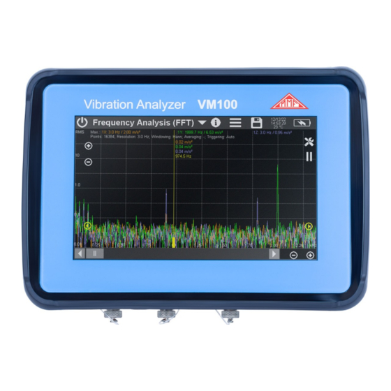
AMPLITUDE/TIME Instr.: VM100A Ser.: 123456 Comment: TEST 2 NFC Id: Sensor 1X: Ser.: 170345 Sensit.: 10.313 mV/m/s² Sensor 1Y: Ser.: 170345 Sensit.: 10.354 mV/m/s² Sensor 1Z: Ser.: 170345 Sensit.: 10.879 mV/m/s² Sensor 2X: Ser.: 181653 Sensit.: 100.45 mV/m/s² Sensor 2Y: Ser.: 181653 Sensit.:... - Page 17 Figure 17: Measurement screen of frequency analysis The frequency range extends up to 22 kHz. The entire screen width of 800 points is used to display the spectrum. At the bottom right, you will see two buttons for zooming in and out of the visible frequency range.
- Page 18 Figure 18: FFT menu The scaling of the amplitude axis can be switched between linear and logarithmic. Windowing determines with which weighting the obtained sample values within a section (window) are used in subsequent calculations. Due to the block-wise pro- cessing of the signal, so-called leakage effects occur on the edges of a block, which make the spectral components appear too wide.
- Page 19 Particularly suitable for closely spaced frequency components Hann Especially suitable for narrowband sinusoidal signals Hamming Particularly suitable for closely spaced frequency components Flattop Especially suitable for measurements with good amplitude accuracy Figure 19: Window functions used in the VM100 (Wikimedia Commons)
- Page 20 Averaging of 2 to 16 spectra can be performed. This can significantly reduce the "noise carpet" contributed by random signal components and improve the sharpness of the displayed spectrum. Averaging has a disadvantageous effect on the reaction time after signal changes. With the key averaging can be restarted.
- Page 21 In the waterfall mode a pseudo-3D graphics is shown for the spectra. In the "back- ground" of the currently measured spectrum, up to 50 previous spectra are dis- played. This can be useful, for example, to make resonance points visible during the run-up or coast-down of a machine (Figure 21).
- Page 22 FREQUENCY ANALYSIS (FFT) Instr.: VM100A Serial no.: 123456 Comment: NFC Id: Sensor 1X: Serial no.: Sensit.: 10.313 mV/m/s² Sensor 1Y: Serial no.: Sensit.: 10.354 mV/m/s² Sensor 1Z: Serial no.: Sensit.: 10.879 mV/m/s² Date: 21.01.2022 Time: 07:36:50 Temp: °C Points: 2048 Window: Hann X: m/s²...
-
Page 23: Module Amplitude/Rotation Speed
3.3. Prerequisite for the measurement is the connection of a photoelectric reflex switch VM100-LS (see Figure 52 on page 41) to the input "RPM" of the VM100, which serves as rotary speed sensor. - Page 24 RPM ramp determines the direction in which the RPM must change in order for the amplitudes to be recorded. The following choices are possible: - Undefined: Both increasing and decreasing speeds are taken into account. - Run-up: Only increasing speeds are taken into account. - Coast-down: Only decreasing speeds are taken into account.
- Page 25 AMPLITUDE/ROTATION SPEED Instr.: VM100A Serial no.: 123456 Comment: NFC Id: Sensor 1X: KS903B10 Ser.: 20014 Sensit.: 10.313 mV/mm/s Sensor 1Y: KS903B10 Ser.: 20014 Sensit.: 10.354 mV/mm/s Sensor 1Z: KS903B10 Ser.: 20014 Sensit.: 10.879 mV/mm/s Sensor 2X: Ser.: Sensit.: 10.000 mV/m/s² Sensor 2Y: Ser.: Sensit.:...
-
Page 26: Module Machine Vibration
An exception is the measurement on reciprocating compressors, where the vibration displacement and vibration acceleration are also recorded. The VM100 also supports the monitoring of roller bearings according to ISO 13373-3 on the basis of RMS and peak values of the vibration acceleration in the frequency range from 10 Hz to 10 kHz. -
Page 27: Measurement Routes
4.5.2. Measurement Routes Machine vibration measurement with the VM100 can be performed with one axis or triaxial with the accelerometer on input 1, channel X or X/Y/Z respectively. Metra recommends rugged, electrically isolated industrial types, such as the single-axis KS80D and KS74C100 or the triaxial KS813B. -
Page 28: Creating Measurement Points In A Route
(Fig- ure 28). To do this, bring the upper left corner of the VM100 close to the NFC tag (see section 5.2). If the NFC tag was recognized, confirm the creation of a new measuring point. The NFC serial number is used as measuring point ID. - Page 29 Figure 30: Adding a new route point A menu opens with the above-mentioned standards and the required selection crite- ria (Figure 31). After the selection has been made, the limit values for warning and alarm are displayed (Figure 32). By touching these are transferred into the mea- suring point menu.
- Page 30 Figure 32: Settings and limit value for the selected standard After closing the measuring point menu with , the newly created measuring point appears with its settings in the measuring route (Figure 33). Figure 33: Measuring route with measuring point...
-
Page 31: Trend Monitoring Of Vibration Severity
4.5.4. Trend Monitoring of Vibration Severity On rotating machines, the RMS value of vibration velocity serves as a monitoring variable for trend recording. For reciprocating compressors, vibration displacement and vibration acceleration are also measured. If a measuring point has been created, measured values can be recorded for trend monitoring. - Page 32 By touching the current measuring values are added to the trend. The VM100 saves the measuring points and their measured values in the TREND folder on the SD card in CSV format. The file name is made from the measuring point ID and the ending “csv”.
- Page 33 The date of the last measurement performed is displayed in the last column of the measurement route for each measurement point. The VM100 uses this date to deter- mine whether it is still within the defined measurement interval (cf. Section 4.5.3) or whether a new measurement is due.
-
Page 34: Roller Bearing Monitoring Using Overall Values
Figure 37: Measurement route with color coded due points 4.5.5. Roller Bearing Monitoring Using Overall Values In addition to monitoring unbalance vibrations, the VM100 supports the monitoring of roller bearings according to ISO 13373-3 based on RMS and peak values of vi- bration acceleration in the frequency range from 10 Hz to 10 kHz. - Page 35 Figure 38: Roller Bearing monitoring to ISO 13373-3 Figure 39 shows an example of stored CSV measurement data of a roller bearing. The columns to the right of the date and time contain the RMS value, the peak value and the resulting alarm limit. The warning limit is 0.56 times the alarm limit. TREND DATA 220217083409 Instr.:...
-
Page 36: Module Envelope Analysis
4.6. Module Envelope Analysis 4.6.1. Introduction Envelope analysis is a method for roller bearing diagnosis. A roller bearing, consist- ing of outer ring, inner ring, rolling elements and cage, generates certain characteris- tic rollover frequencies during when rotating, which are by their design in a rela- tionship to the rotor rotational frequency. - Page 37 Figure 41: Measurement view of envelope analysis The entire screen width of 800 points is used to display the envelope spectrum. At the bottom right, you will see a plus or minus button for zooming in or out of the visible frequency range.
- Page 38 Select RPM sensor if you can measure the speed. The prerequisite for this is the connection of a VM100-PS photoelectric reflex switch to the "RPM" input of the VM100 and the attachment of a reflective label on the rotor.
- Page 39 Figure 43: Bearing list Touch to add a new bearing. A menu opens for entering the damage frequencies (Figure 44). Figure 44: Entering damage frequencies The bearing name and the damage frequencies are entered by touching the corre - sponding input field using the screen keyboard. The damage frequencies are entered as factors relative to the rotational frequency as unitless values.
- Page 40 the rotational frequency. The measured or entered rotational speed can be found in line 18. From line 20 the frequency points and the corresponding amplitudes follow. The number of lines depends on the selected resolution. ENVELOPE ANALYSIS Instr.: VM100A Serial no.: 123456 Comment: NFC Id:...
-
Page 41: Module Balancing
4.7. Module Balancing 4.7.1. Introduction Unbalance occurs when masses rotate whose center of gravity is not on the axis of rotation. A centrifugal force is generated in the direction of the unbalanced mass (Figure 46). This centrifugal force increases with the square of the rotational speed. Figure 46: Unbalanced rotor Figure 47: Balanced rotor This results in vibrations, which are often undesirable because they impair product... - Page 42 In addition to one or two accelerometers, a rotation speed sensor is required to pro - vide the angular information for balancing. The VM100 supports field balancing which means the rotor can remain in its in- stalled state and does not need to be transported to a balancing bench. Operational balancing proceeds in the following steps: 1.
-
Page 43: Measurement
The sensors are mounted radially to the axis of rotation, ideally directly on the shaft bearings. At the VM100 the sensors are connected to the measuring channels 1X and 1Y. In the operating dialog, the sensor positions are designated as plane A and plane B. - Page 44 The following example shows the procedure for one-plane balancing. Balancing begins with the initial unbalance run. After the accelerometer and the RPM sensor have been mounted, start rotation. The VM100 measures the speed and...
- Page 45 Figure 54: Initial run (1 plane) After standstill, the VM100 switches to the test run. The measured initial unbalance is displayed as "O" mark in the polar diagram (Figure 55). You are prompted to ap- ply a test mass. If the rotor mass was specified in the settings, a suggestion for the test mass based on a balance quality of 6.3 according to ISO 1940 can be given.
- Page 46 Figure 55: Attaching a test mass (1 plane) Figure 56: Test run (1 plane) After standstill, you will be asked whether the test mass should remain on the rotor (keep) or be removed again (Figure 57). Keeping the test mass can be useful, for ex- ample, if it has been welded on.
- Page 47 Figure 57: Keep or remove test mass (1 plane) The unit now displays the required corrections (Figure 58). You have the option of adding or removing masses only at specified fixed angle positions. This can be use- ful, for example, on fan wheels with a certain number of blades. Check the box and enter the desired number of angles.
- Page 48 Figure 58: Corrections (1 plane) Once the corrections have been made, confirm with and start the rotor for the check run (Figure 59). You will see the resulting unbalance vector. Under ampli- tude and angle, the difference to the original state is displayed as a percentage. It provides information about the balancing progress.
- Page 49 Figure 59: Check run (1 plane) Figure 60: Continue or finish...
- Page 50 Two-plane balancing is performed in a similar way. In addition, a second test mass is applied and a second test run is performed for plane B. The following is a brief description of the procedure based on an example. First, the unbalance for both planes is measured in the initial condition (Figure 61). Figure 61: Initial run (2 planes) This is followed by the application of a test mass in plane A and a restart of rotation (Figure 62).
- Page 51 The results of the test run at plane A are saved (Figure 63) and rotation is stopped. Figure 63: Test run of plane A (2 planes) Now decide whether you want to leave the test mass on the rotor or remove it again (Figure 64).
- Page 52 Then place a test mass in plane B and start rotation again (Figure 65). Figure 65: Attach a test mass for plane B (2 planes) Test run B is performed. After saving and stopping the rotation, confirm that you have removed or left the test mass in plane B (Figure 66). Figure 66: Confirm keeping or removing the test mass B (2 planes)
- Page 53 Now the calculated correction masses and their angles are displayed for both planes (Figure 67). In the example, 16 angular steps (fixed locations) were selected. Figure 67: First correction (2 planes) Make the corrections and confirm. Start rotation for the first check run (Figure 68). Figure 68: First check run (2 planes) Unbalance (U) in the selected unit of measurement and balance quality (G) accord - ing to ISO 1940 for both planes are displayed below the diagram.
- Page 54 After saving the result and stopping the rotation, you will be asked whether you want to finish or continue the balancing process here (Figure 69). Figure 69: Continue or finish balancing after first check run (2 planes) In this example, balancing is continued. Further corrections for both planes are dis- played (Figure 70).
- Page 55 In the second check run, there has been another improvement. In the polar diagrams, the numbered vectors of the check runs are displayed next to the initial unbalance (Figure 71). Figure 71: Second check run (2 planes) the correction masses applied to each plane can be combined into one mass or, in the case of angle fixed positions, into two masses (Figure 73).
- Page 56 Figure 73: Combination of corrections (2 planes) opens a text window with a summary of all changes made and the resulting vi- bration or unbalance vectors (Figure 74). Figure 74: Auswuchtprotokoll To save this report, touch and select Save CSV balancing report. An example of a saved CSV file is shown in Figure 75.
- Page 57 Alternatively, the display content can be saved as BMP screenshot. The files are found on the SD card in the "BAL" folder. BALANCING REPORT Instr.: VM100A Ser.: 123456 Sensor A: Ser.: Sensit.: mV/ms^-2 Date & Time: 10/02/22 13:55:52 Temp: °C Comment: NFC Id: Balancing mode:...
-
Page 58: Module Third Octave Analysis (Vc And Nano Criteria)
4.8. Module Third Octave Analysis (VC and Nano Criteria) 4.8.1. Introduction This module is used for vibration measurements on very sensitive equipment, e.g. electron microscopes, photo-lithography equipment or microelectronics and nan- otechnology equipment. In order to standardize the installation and operating condi- tions of these systems, so called VC limits (Vibration Criteria) were developed in the 1980s. - Page 59 Vibration Amplitude in Third Structure Application Criterion Octave Spectrum size Very hard to observe criterion for 1.6 µm/s REMs in nanotechnology, top 1 to 5 Hz and Nano-D floors with high requirements re- 1 nm 6.4 µm/s garding dynamic stiffness and natu- 20 to 100 Hz ral frequency Extreme criterion for REMs in nan-...
-
Page 60: Sensors For Vc And Nano Criteria
4.8.2. Sensors for VC and Nano Criteria This measurement has the highest demands in terms of resolution and noise for used vibration transducers. Only piezoelectric accelerometers with high sensitivity can be considered. Figure 77: Triaxial Figure 78: Uniaxial ac- Figure 79: Uniaxial accelerometer KS823B accelerometer KB12VD celerometer KS48C... -
Page 61: Measurement
80 % of the limit value. Between 80 and 100 % the indicator is yellow, above that red. Always disconnect the VM100 from the USB port during high-sensitivity mea- surements to avoid interference. - Page 62 Use the button to open the settings menu (Figure 83). Figure 83: Menu for settings Figure 84: Menu for custom limits In the Limit line menu, select the required vibration criterion. In addition to the VC and Nano criteria, it is also possible to define your own limit values. To do this, se- lect "Custom", whereupon the menu for entering the limit values opens (Figure 84).
- Page 63 Figure 86: Spectrum with held maximum values The Save mode menu has two options: • Limit line: Each time the spectrum crosses the limit line a measurement is saved. Touch to open the save menu and select Save CSV. You may enter a file name or use the default name composed of date and time (example: “OCTAVE_220607_100645.csv”).
- Page 64 Figure 87: CSV formatted third-octave data (only left part shown) For more information on storing measured values, refer to section 5.
-
Page 65: Module Hand-Arm Vibration
4.9. Module Hand-Arm Vibration 4.9.1. Introduction This module supports the measurement of hand-arm vibrations according to ISO 5349 and VDI 2057 with one or two hands. These are vibrations that are intro- duced into the body via the hand. They can cause, for example, circulatory diseases, bone or joint damages and muscle disorders. - Page 66 √ A(8)=a Equation 1 where A(8) is the daily exposure is the energy equivalent mean value of the frequency weighted acceleration during exposure, which means the vector sum of Wh frequency-weighted RMS values in the directions X/Y/Z √ Equation 2 is the total duration of exposure during one work day is the reference duration of 8 hours The daily exposure value can be composed of several exposure sections with differ-...
- Page 67 10,0000 Wh max Wh min Wh VM100 1,0000 0,1000 0,0100 0,0010 0,0001 1000 10000 Figure 88: Frequency weighting Wh...
-
Page 68: Hand-Arm Sensors
4.9.2. Hand-Arm Sensors Metra recommends the KS963B10 triaxial accelerometer for hand-arm measurements. Select a measurement point that is as close as possible to the gripping points of the hand, but without interfering with the normal working process. The measurement should be made using forces that correspond to typical op- erating conditions. -
Page 69: Measurement
They are used to calculate the daily exposure value A(8) (cf. Section 4.9.1). Based on the higher of the two energy-equivalent mean values, the VM100 calculates the exposure time at which the action value and the exposure limit value according to EU Directive 2002/44/EC would be reached. - Page 70 Figure 93: Measurement screen for hand-arm vibration Measuring value can be stored as CSV data table. To do this, open the storage menu with and select Save CSV (see section 5). The save button then appears in yel- low with the text "LOG" on it. The measured values are now written to a file every second.
- Page 71 HAND-ARM VIBRATION Instr.: VM100A Ser.: 123456 Comment: NFC Id: Sensor 1X: KS963B10 Ser.: 20013 Sensit.: 10.221 mV/ms^-2 Sensor 1Y: KS963B11 Ser.: 20013 Sensit.: 10.154 mV/ms^-2 Sensor 1Z: KS963B12 Ser.: 20013 Sensit.: 10.167 mV/ms^-2 Sensor 2X: KS963B13 Ser.: 20014 Sensit.: 10.313 mV/ms^-2 Sensor 2Y: KS963B14...
-
Page 72: Module Whole-Body Vibration
4.10. Module Whole-Body Vibration 4.10.1. Introduction This module supports the measurement of whole-body vibrations according to ISO 2631. These are vibrations acting over the buttocks and back of the seated per - son, the feet of the standing person and the head and back of the lying person. These can lead, for example, to back pain and damage to the spine. - Page 73 X/Y/Z directions. The largest of the three values is used for risk assessment, i.e. compared with limit values according to the EU Directive. √ ∑ (8)= Equation 5 √ ∑ (8)= Equation 6 √ ∑ (8)= Equation 7 where: are the daily exposure values for direction X/Y/Z x/y/z are the energy equivalent mean values (a ) for acceleration in directions...
-
Page 74: Whole-Body Sensors
√ ∑ iexp (8)= ⋅ Equation 9 imeas √ ∑ iexp (8)= ⋅ Equation 10 imeas √ ∑ iexp (8)= ⋅ Equation 11 imeas where are the daily exposures of directions X/Y/Z X/Y/Z are the frequency-weighted vibration dose values of directions X/ x/y/zi Y/Z during exposure section i is the duration of exposure section i... - Page 75 Figure 96: Coordinate systems for whole-body vibration to ISO 2631 Whole-Body Health Evaluation Frequency Weighting Posture Position Direction weighting factor (k) X / Y sitting seat surface Whole-Body Comfort Evaluation X / Y seat surface X / Y 0.25 feet platform sitting backrest X / Y...
- Page 76 When measuring whole-body vibrations, the frequency range from 0.4 to 100 Hz is considered. Depending on the application, different weighting filters are used. Fig - ures 97 to 101 show the frequency weightings implemented in the VM100. 10,000 Wd min...
- Page 77 Wj min Wj max Wj VM100 0,01 0,001 0,0001 1000 Figure 99: Weighting filter Wj Wd min Wd max Wd VM100 0,01 0,001 0,0001 1000 Figure 100: Weighting filter Wc...
-
Page 78: Measurement
Wm min Wm max Wm VM100 0,01 0,001 0,0001 1000 Figure 101: Weighting filter Wm 4.10.3. Measurement Figure 102 shows the measurement screen of the whole-body vibration module. In the upper section is the uniform menu bar described in section 3.3. On the top left, the selected evaluation (health or comfort) is displayed. - Page 79 Below the largest of the three axis values is displayed, which is used to calculate the daily exposure value A(8) according to ISO 2631 (cf. Section 4.10.1). From this, the VM100 calculates the exposure time at which the action value and the exposure limit value according to EU Directive 2002/44/EC would be reached. In addition, the elapsed measuring time is displayed.
- Page 80 A measurement always starts by touching the reset button . This restarts the calculation of interval RMS values and resets the measurement duration timer. Use the button to open the menu for settings (Figure 103). Here you define whether a measurement is performed for health or comfort evaluation. In addition, you can switch between RMS value and vibration dose value (VDV) (cf.
- Page 81 WHOLE-BODY VIBRATION Instr.: VM100A Ser.: 123456 Comment: NFC Id: Sensor 1X: KS903B10 Ser.: 20014 Sensit.: 10.313 mV/ms^-2 Sensor 1Y: KS903B10 Ser.: 20014 Sensit.: 10.354 mV/ms^-2 Sensor 1Z: KS903B10 Ser.: 20014 Sensit.: 10.879 mV/ms^-2 Date: 25.01.2021 Temp: °C Channel: Filter: Factor: Jan 40 Jan 40 1.00...
-
Page 82: Module Whole-Body - 3 Sensors
4.11. Module Whole-Body – 3 Sensors 4.11.1. Introduction This module is used to evaluate ride comfort in motor vehicles in accordance with GB/T 4970-2009. It is based on the measurement of whole-body vibrations in ac - cordance with ISO 2631. In this case, the vibrations on the seat surface, the seat back and the foot platform are measured simultaneously when driving along a speci- fied test track. -
Page 83: Measurement
4.11.3. Measurement 102 shows the measurement screen in the whole-body vibration module. In the up- per section you see the uniform menu bar as described in section 3.3. Figure 106: Measurement screen in the whole-body vibration mode with 3 sensors On the left, the vibration values for the measurement positions Seat, Backrest and Feet are output for three axis directions each. - Page 84 Z-axis is perpendicular to the backrest and therefore also to the spine. To es- tablish the correct axis assignment, the weighting filters and factors for X and Z are swapped in the VM100 for measurements on the backrest. The alignment of the measuring axes in the measuring positions can be found in Figure 96 on page 73.
- Page 85 Figure 107: Comfort zones A measurement always starts by touching the reset button . This restarts the calculation of the interval RMS values and resets the measurement timer. The measured values can be stored as CSV data table. To do this, press to open the storage menu and select Store CSV (see section 5).
-
Page 86: Saving Measurements And Nfc Function
The text-based files can be imported into spreadsheet programs. WAV (WAVE) is a format for audio files. It is used in the VM100 for raw data. WAV files can be opened in audio players and imported into many signal analysis programs. -
Page 87: Nfc Identification Of Measuring Points
The VM100 reads NFC tags of types, A, B, F and V. Each NFC tag contains a unique serial number, which the VM100 uses for identification. Other NFC func- tions are not used. -
Page 88: Saving Bitmap Screenshots
Figure 110: NFC detection and sensitive corner If desired, you can assign a plain text name to it. The input field to the right of the serial number is used for this purpose. This text will then also be displayed the next time the NFC tag is recognized. -
Page 89: Saving Data In Csv Format
It can be opened in spreadsheet programs, for example. The chapters on the measurement modules show examples of this. The VM100 uses the semicolon as separator. The files always consist of a header, which contains information about the sensors, the device and selected settings. - Page 90 As file name you can use either the name suggested by the instrument with date and time or enter a name yourself. For the actual file name the VM100 adds the measur - ing channel, e.g. "C1X" and the selected gain, e.g. "G100". The complete file name is then for example "210104_045152C1XG100.wav".
- Page 91 Figure 114: Raw data saving Section 3.5 describes how you can transfer the data stored on the SD card to a PC via the USB interface.
-
Page 92: Presets
6. Presets You can save up to 10 sets of settings for faster access. This is done in the main menu under "Presets". All current menu settings including the settings of the measuring graph are saved. Figure 115: Saving and loading settings In the delivery state, all entries are empty. -
Page 93: Other Settings
7. Other Settings 7.1. Display Settings Touch the button and open the main menu to select Settings and Display (Fig- ure 116). Figure 116: Display settings Touch Brightness to open the menu for set- ting the display brightness (Figure 117). The share of the backlight can be up to 50 % of the total power consumption of the device. -
Page 94: Date And Time
Figure 120: Date and time 7.3. Language In Figure 121 you can see how to select the display language of the VM100. The selection of the language only affects the operating dialog. All stored data remains in English. Figure 121: Display language selection 7.4. -
Page 95: Firmware Update
Windows systems with 32 and 64 bit. Unpack and install the software on your You can also obtain the current firmware file vm100.zip from our download page. Unpack the contained file vm100.hex and save it in a folder of your choice. ➔ Please follow the instructions below exactly. The firmware update affects mem- ory sectors 2 to 7. - Page 96 Figure 125: STM32CubeProgrammer with loaded firmware file Now the VM100 needs to be prepared for the update. To do so, switch the VM100 off. Unscrew the cover of the update interface (Figure 126). Connect the USB-C up- date interface to a PC (Figure 127).
- Page 97 Click the button under “USB” to refresh the dis- play. If the VM100 is recognized by the PC as a DFU device, it will appear in the update program as port "USB1" (Figure 130). Click button starts the firmware transfer to the VM100.
- Page 98 Figure 131: Finished firmware update...
-
Page 99: Technical Data
Measurement Modules Amplitude/time VM100-AMP (pre-installed) Frequency analysis VM100-FFT (pre-installed) Amplitude/rot. speed VM100-RPM (option) Machine vibration VM100-MACH (option) Envelope analysis VM100-ENV (option) Balancing VM100-BAL (option) Third-octave analysis VM100-VC (option) Hand-arm VM100-HA (option) Whole-body VM100-WB1 (option) Whole-body-3 sensors VM100-WB3 (option, only for VM100A) - Page 100 Overall value measurement in time domain and human vibration (VM100-AMP / VM100-HA / VM100-WB1 / VM100-WB3) Channels 1 to 9 1 to 3 Measurands Acceleration; velocity (<4 kHz); displacement (<300 Hz) Overall values Interval RMS (unlimited), RMS (1s), peak value,...
- Page 101 Machine Vibration (VM100-MACH) Channels 1 to 3 Measuring routes Measurement point description with location, machine, position and comment; automatic detection with NFC tags Trend view Amplitude time graph with limit lines ISO standard assistant ISO 20816-2: Gas and steam turbines >40 MW ISO 20816-3: Industrial machines >15 kW...
- Page 102 Optional Accessories Sensor adapter cable 034-B711-BNCf: Binder to BNC female; 0.5 m Photoel. reflex switch VM100-PS...
- Page 103 Limited Warranty Metra warrants for a period of 24 months that its products will be free from defects in material or workmanship and shall conform to the specifications current at the time of shipment. The warranty period starts with the date of invoice. The customer must provide the dated bill of sale as evidence.
Need help?
Do you have a question about the VM100 and is the answer not in the manual?
Questions and answers