Table of Contents
Advertisement
Quick Links
Advertisement
Table of Contents

Related Manuals for Correlated Solutions Vic-3D 8


Summary of Contents for Correlated Solutions Vic-3D 8
- Page 2 1394b connection. Always check orientation and compatibility before making any connection. • For any test where excessive heat, shock, or flying debris may be present, take steps to protect the cameras and equipment. Various shielding solutions are available – please contact Correlated Solutions for more details.
- Page 3 INTRODUCTION Completing a test with Vic-3D is fairly straightforward but a few pointers can help to get the best results in the shortest period of time. This document explains the basics of a test from start to finish. A typical sequence will be: •...
-
Page 4: Setting Up The Cameras
SETTING UP THE CAMERAS POINTING THE CAMERAS To begin, set your prepared specimen in its testing location. Be aware of the orientation and potential camera placement; for example, for a dog-bone specimen in a test frame, the prepared face of the specimen should face outwards from the test frame rather than facing the frame’s columns. - Page 5 The distance is set so that the specimen roughly fills the field of view. If the specimen is larger than the field of view, we lose data at the edges; if the specimen is much smaller, our spatial resolution suffers. Note that the entire area of interest must be visible in both cameras –...
-
Page 6: Adjusting Focus
Once a lens and approximate distance is selected, the cameras can be pointed. The cameras should be positioned somewhat symmetrically about the specimen; this will keep the magnification level consistent. The exact angle included between the cameras is not critical but selecting a correct stereo angle will give best results: the angle should be at least 25º... - Page 7 APERTURE AND EXPOSURE TIME As you make the image sharp through the focus adjustment, it will also be necessary to adjust the brightness of the image. There are two controls available for this: the aperture/iris setting on the lens, and the exposure time setting of the camera. •...
- Page 8 This lens has an aperture ring with a locking knob. To focus, loosen the collar (for this particular lens, a 2mm hex driver is used), and rotate the entire body of the lens. Loosen the lens body (counterclockwise) to focus closer; tighten (clockwise) to focus farther.
- Page 9 TO CONCLUSIVELY CHECK FOR HEAT WAVES, YOU CAN SIMPLY TAKE SEVERAL IMAGES OF THE SAME SCENE (NO LOAD/MOTION) AND RUN THEM. IF HEAT WAVES ARE PRESENT, YOU WILL SEE LARGE DISPLACEMENT FIELDS THAT CHANGE RANDOMLY FROM IMAGE TO IMAGE. Once the camera positions have been set and the focus and aperture adjusted, calibration can begin. After this point, changing any aspect of the camera system will invalidate the calibration;...
-
Page 10: Analog Data
ANALOG DATA For systems equipped with data acquisition hardware, several channels of analog data may be acquired along with the image data. To view the analog data, click the Analog Data button in the toolbar. (If this button is not present, analog acquisition is not installed. - Page 11 CALIBRATION SELECTING A GRID To begin, select a grid that approximately fills the field of view. Too large Correct Too small If the grid is too large, it will be difficult to keep it fully in the field of view in both cameras while taking images. However, calibration images will be useful as long as all three of the hollow marker dots are visible.
- Page 12 ACQUIRING GRID IMAGES Before acquiring calibration images in Vic-Snap, select a name for the images by clicking Edit Project in the menu or toolbar. A consistent suffix such as “cal” will make future reference easier. In this case, we’ll be keeping both the calibration and test images together in a folder called “bending-test”.
- Page 13 CALIBRATION IN VIC-3D To calibrate using the acquired grid images, start Vic-3D. Select Calibration images from the start page, or click Project… Calibration images. Navigate to the correct folder and select all your calibration images; click Open. The selected images will appear under the Calibration Images section in the Images tab. To begin calibration, click the Calibrate button in the toolbar, or select Calibration…...
- Page 14 For each image, a number of points extracted is displayed. When the extraction is complete, the calibration will be computed; a score will be displayed for each image; and a final score displayed in the lower right. IMAGING SYSTEM AND DISTORTION ORDER To edit the characteristics of the imaging system model, click Edit by the imaging system drop-down menu.
- Page 15 For lenses with higher distortion orders, more images may be required, and it becomes even more important to take grid images where points are present in the corners of the field of view. As many as 30 images may be required to accurately estimate 3 order distortions.
- Page 16 • The grid is rigid. The grid is evenly lit. For a backlit glass grid, this is particularly important. • • If using a glass grid, confirm the correct face is towards the camera. • The cameras are synchronized. • Correct any potential problems and recalibrate.
-
Page 17: Running The Test
RUNNING THE TEST Once calibration is complete, you may run the test. (Note that you may proceed directly from acquiring calibration images to acquiring test images. However, you may not uncover any problems with the setup until it is too late. For important tests, you should check the calibration before testing.) Double-check the position of the specimen and stereo rig;... - Page 18 Note: even for timed capture tests, you may want to acquire and analyze a single static image of the specimen before running the test. This will verify that the test is ready to proceed and there are no problems with the lighting, calibration, focus, or speckle pattern.
- Page 19 CORRELATION IN VIC-3D SPECKLE IMAGES If you closed Vic-3D before acquiring test images, re-open it; then, select the saved project file with the calibration from the start page, or use File… Open. Next, add the speckle images. Select the speckle image tool or click Project… Speckle Images. Select the desired images.
- Page 20 DEFINING THE AOI Before running the correlation, we have to define an area of interest (AOI). This is the portion of the image that contains the speckle pattern and which will be analyzed for shape and displacement. To begin, double-click on the reference image to open the AOI Editor.
- Page 21 Next, set the Subset and Step for this AOI. The default values work well for most speckle patterns. If the pattern is very coarse, larger subset values may be needed. To run a very fast analysis of many images, increase the step to 10 or 15. If multiple speckle areas are present, you may draw as many additional AOI’s as necessary.
- Page 22 Double-click on the new start point to open the Initial Guess Editor. In this case, the initial guess has been automatically found – the areas at the top right match, and the indicator next to each image is green. At this point we could click Done and continue to the analysis. If an initial guess is needed, we provide it by pointing to matching spots in the left and right image, as well as the deformed images, if necessary.
- Page 23 CORRELATION OPTIONS In the Files tab, you can select files to analyze (note: the reference image is always analyzed.) Right click in the list to select only certain images. In the Options tab, you can fine-tune correlation options. One useful setting is incremental correlation. This correlates each image to the prior image rather than always correlating to the reference image.
- Page 24 The Thresholding tab allows you to set the limits beyond which data will be discarded (leaving ‘holes’ in the plot). Raising a threshold will always allow more data. • Prediction margin: discards points that are inconsistent with neighbors. This is the most useful threshold for limiting false matches.
- Page 25 The Post-Processing tab allows you to control how the data is processed immediately after calculating. To calculate strain during the correlation, rather than after (so you can see it in the preview), check the Strain Computation box. Frequently none of the options or thresholds will need to be changed. In this case, simply click Run to start the analysis, click Run.
- Page 26 Alternately, if the error is high and the plot shows obviously erroneous data in one region (spikes/noise), there may be a problem with the analysis in that region; check the images and AOI boundaries. If necessary, reduce the analysis area, or use threshold settings to eliminate the bad data.
- Page 27 VIEWING AND REDUCING DATA VIEWING FULL-FIELD DATA When the analysis is complete, click Close. The new data will be displayed in the Data tab at left; double click on a file to view. You can click and drag to rotate the data set and use the mouse wheel to zoom in and out. Right click to select different contour variables.
- Page 28 To edit axis and contour limits, use the Plotting tools toolset, at the left. You may either auto-scale the axis and contour limits or clear the Auto-rescale box and manually enter limits. To animate through the images, use the Animation toolbar: Or, videos can be exported by right-clicking in the plot and selecting Export video.
- Page 29 You can calculate strain for all files by clicking Start. Alternately, you can adjust settings and see the effect on a single file by clicking Preview. After strain calculation is complete, there will be new strain variables in the data set; right-click on the contour plot to view them.
- Page 30 Next, click the Plot extractions button (farthest right) in the Inspector toolbar. A time series plot appears: The default sets are the average for the whole field, as well as any inspectors you have placed (here, P0, the inspection point). You can zoom in and move around the plot with the mouse. You can also change the settings and appearance with the right-click menu.
- Page 31 To change the variables and series plotted, use the toolbar at the top left. You can add and remove a series by clicking Add or Delete. To edit a series, click on it and select different variables: Click the ↵ button next to each line to commit the change. To save this extraction from one or many of the data files, click Export, or save an image of the plot by right-clicking in the plot and selecting Save plot.
- Page 32 You may also extract a slice of data with the Extract Line tool on the toolbar. Click the tool and then click two endpoints to define a line: Then, click the Plot extractions button on the Inspector toolbar. Now, you can pull down in the extraction tools to select line slices:...
- Page 33 This will display the data along the line for each image. By default, several data files are shown, and the currently selected file is plotted as red. You can right-click and access the Settings dialog to change to plot only the selected file, or only certain files. As before, this data can be exported or the plot saved.
- Page 34 Then, click the Plot extractions button. A third option is now available on the pulldown – extensometers. Allowable data sources for the extensometer are ∆L/L0 (engineering strain), ∆L (difference in length), L1 (deformed length), and L1 (initial length). Note that this tool gives simple end to end distances, which may not always be the same thing as strain –...
- Page 35 SUPPORT If you have any questions about this document or any other questions, comments, or concerns about our software, please feel free to contact us at support@correlatedsolutions.com, or visit our web site at www.correlatedsolutions.com. APPENDICES • Stereo camera mounting instructions AN-722: External Orientation Calibration •...
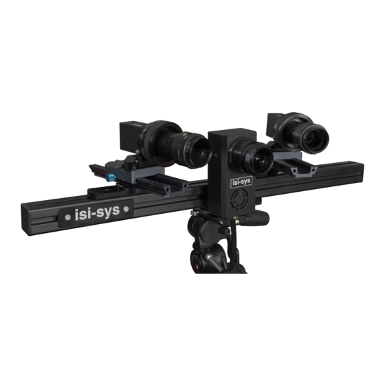
- Page 36 STEREO CAMERA MOUNTING INSTRUCTIONS Items List: A. Tripod B. Tripod 3-axis adjustable head C. Tripod quick-release adapter D. Slide block E. 23” Aluminum profiles F. Adjustable extrusion mounting hinge G. Camera FLEX mounts H. Extrusion profile end caps Tools required: I.
- Page 37 Figure 1. Items List Set up tripod Pull the three legs outward to the desired location b. Unlatch each leg and raise to the approximate desired height Lock them back so the tripod is stable.
- Page 38 Figure 2. Tripod There is an option whether to incorporate the tripod 3-axis adjustable head in the setup. The tripod head allows for additional degrees of freedom and more adjustability. However, the more degrees of freedom that are present in the system, the less rigid the system is.
- Page 39 Screw the tripod 3-axis head onto the tripod. Make sure the handles are attached. Figure 3. Trip with 3-axis head/bracket assembly Snap the quick-release bracket to the tripod 3-axis adjustable head. Figure 4: Quick-release bracket...
- Page 40 a. To fasten the slide block to the tripod 3-axis adjustable head, verify that there is a helical insert present in the slide block. This will allow the slide block to screw directly onto the tripod head. Figure 5. Slide block with helical insert Screw the slide block onto the tripod 3-axis adjustable head.
- Page 41 Figure 7. Slide block without helical insert Figure 8. Slide block mounted to tripod Carefully slide one of the 23” aluminum extrusion pieces into the slide block about halfway (the handle/T-nut may need to be loosened in order to be to do this), and then hand tighten the handle on the side of the block to fasten the extrusion in place.
- Page 42 Figure 9. Aluminum extrusion on slide block Attaching the hinge Loosen the T-nuts on the mounting hinge so that they will slide into the slots of the extrusion. Orient it so that the silver inserts on the hinge go through the slot of the extrusion. b.
- Page 43 Figure 10. Hinge mounted to extrusion Tighten the T-nut with the provided 5mm hex driver so that the hinge is close to the end of the extrusion. d. Slide the other 23” extrusion piece through the hinge’s other T-nut about halfway so that it is perpendicular to the already mounted extrusion bar, as seen in Figure 11.
- Page 44 Figure 11. Hinge attaches aluminum extrusions Attaching the camera/swivel mounting assembly Each swivel mount has two T-nut fasteners. b. Loosen the T-nuts so that they will slide into the slot of the extrusion. Slide the swivel camera mounts to the desired position on the extrusion bar. d.
- Page 45 Figure 12. Mounting the camera/swivel assembly...
- Page 46 Attach the 4 end caps to the aluminum extrusion ends. Figure 13. Attach all four end caps Adjust all degrees of freedom to the desired locations and tighten. Other mounting configurations are shown in Figures 14 and 15. Figure 14 displays the final configuration when the tripod head is omitted.
- Page 47 Figure 14. Complete system with omitting tripod head Figure 15. Complete system with vertical camera mounting...
- Page 48 CSI APPLICATION NOTE AN-722 EXTERNAL ORIENTATION CALIBRATION IN VIC-3D INTRODUCTION Calibration in Vic-3D serves to establish two distinct sets of parameters. • Intrinsic parameters: These parameters are specific to each camera. We calculate focal length, aspect ratio, and sensor center (the point on the sensor that corresponds to the center of the lens). These parameters will change if you move the lens or change the aperture or focus.
- Page 49 PROCEDURE 1: CALIBRATING SEPARATELY Select Calibration… Calibrate Camera 1 from the menu bar. Proceed as with stereo calibration; repeat for Camera 2. At this point, you may check the Calibration tab at the left side of the main window and confirm that both cameras are calibrated but the Transformation section shows “Not calibrated”.
- Page 50 Load this image pair as the Reference image, as normal. Define an area of interest that contains the two measurement marks and encompasses as much of the shape as possible. Using a patch that is too narrow or small may result in erroneous results.
- Page 51 Click Calibration… Calibrate camera orientation on the menu bar. You will see your reference image; where data is present, the image is overlaid with blue. Click on one of your measurement marks, and then the other. You will be asked to enter the distance between these points to establish scale: Enter the previously measured distance.
- Page 52 The calibration is now complete. If desired, you may note the figures in the Transformation section of the Calibration tab and confirm that they are as expected. Alpha, Beta, and Gamma are the three angles between the cameras; Tx, Ty, and Tz are the displacements;...
- Page 53 PROCEDURE 2: CALIBRATING TOGETHER To calibrate as a system and then refine the calibration with External Orientation Calibration, begin by calibrating as normal (Data… Calibrate… Calibrate Stereo System). Load a reference image and select an AOI that covers as much of your specimen as possible. If desired, check the initial guess.
- Page 54 NOTE: THE FIXED BASELINE METHOD WORKS BY ASSUMING THAT THE DISTANCE BETWEEN CAMERA SENSORS HAS NOT CHANGED. THIS IS A GOOD APPROXIMATION WHEN THE CAMERAS ARE IN A TYPICAL MOUNTING CONFIGURATION WHERE THEY MAY BE ABLE TO ROTATE BUT NOT TRANSLATE. IF THE CAMERAS HAVE MOVED IN A DIFFERENT WAY WHERE THE BASELINE CHANGES SIGNIFICANTLY, THIS PROCEDURE CAN CAUSE SCALE ERRORS IN YOUR RESULTS.
- Page 55 APPLICATION NOTE AN-708 VIBRATION MEASUREMENTS WITH THE VIBRATION SYNCHRONIZATION MODULE INTRODUCTION The vibration module allows complete analysis of cyclical events using low-speed cameras. This is accomplished by locking on to a drive or response signal, and taking images at user-defined phase intervals. Since the camera’s frame rate may not be fast enough to image several times during a single cycle, we may skip several cycles before advancing to the next phase, but the signal is accurately tracked by the phase locking logic.
-
Page 56: Connecting The System
Applications for the module include: • Tire and wheel testing Piston engines • • Speakers Flow-induced vibration • Shake table tests • • Fatigue testing NECESSARY EQUIPMENT/SOFTWARE Making measurements with the vibration module requires only the module, a standard Vic-3D system, and a facility for triggering the system’s cameras. -
Page 57: Test Setup
TEST SETUP Setting up for a vibration test begins with pointing and focusing the cameras, as with a quasi-static test. There is only one major additional concern – lighting. It will be necessary to calculate, or establish empirically, the exposure time required to freeze your motion. -
Page 58: Software Controls
SOFTWARE CONTROLS To being a measurement, start Vic-Snap and click the Fulcrum Dialog toolbar button, or select File… Fulcrum Dialog. The Fulcrum control will appear in the workspace, and the cameras will be switched to hardware trigger mode. The (1.0 s) indicates that the signal is initially being sampled for 1.0 seconds to determine the levels. This time will be determined by the minimum frequency setting in the Advanced Options;... - Page 59 If the signal cannot be locked, the frequency box will display “---”, and a piece of the waveform will be displayed to assist in diagnosis.
- Page 60 Once running, the cameras will be triggered at the specified phase (0º, to start). To change the phase that you are viewing, you can select a different value in the Phase control. The step for this control is determined by the Step control. A sample waveform is displayed at bottom.
-
Page 61: Recording Images
RECORDING IMAGES There are several options for recording images in the vibration module. Since the cameras are hardware triggered, always at the selected phase, you can simply use the space bar to capture individual images, as well as the timed and streaming capture modes. -
Page 62: Usage Scenarios
USAGE SCENARIOS CYCLICAL TESTING In this type of test, the Record Sequence button can be used to acquire a full sequence. Be sure that the specimen is in a stable-repeating mode before you start acquiring; acquire your sequence using whichever step you desire. You may wish to acquire multiple sequences for a given test;... - Page 63 Then, use the Cycle recording interval in the Fulcrum dialog to record at set intervals. You can also use Timed Capture for this. For this kind of test the reference image will typically be taken with the specimen unloaded or slightly preloaded, in order to give strains relative to a relaxed state.
-
Page 64: Setting Advanced Options
SETTING ADVANCED OPTIONS Some adjustments will be found in the Advanced Options dialog (under File… Advanced Options), in the Fulcrum tab. • Default output state: this controls the level of the output trigger signal in between triggers; high is TTL high, low is TTL low. -
Page 65: Theory Of Operation
THEORY OF OPERATION The vibration system operates by setting an analog trigger and window in the hardware DAQ device. This provides the basis of the trigger detection. To provide the phase delay, the measured period is multiplied by the selected phase to establish the delay. -
Page 66: Appendix 1 - Hookup Diagram (Usb Device)
Appendix 1 – Hookup diagram (USB device) AI0. Set to ‘FS’ and connect input signal. USER1. Connect to camera trigger input. -
Page 67: Appendix 2 - Hookup Diagram (Pci Device)
Appendix 2 – Hookup diagram (PCI device) AI0. Set to ‘FS’ and connect input signal. CTR0OUT. Connect to camera trigger input. -
Page 68: Appendix 3 - Hookup (Trigger To Cameras)
Appendix 3 – Hookup (trigger to cameras) ATB-5 Trigger box BNC cable to trigger output Trigger to camera (CSI trigger cables) With ATB-5 BNC Tee BNC cable to trigger output Trigger to camera (Manufacturer BNC to trigger cables) Direct connection... - Page 69 CSI APPLICATION NOTE AN-1701 SPECKLE PATTERN FUNDAMENTALS INTRODUCTION In digital image correlation, using an optimal speckle pattern is one of the most important factors in reducing measurement noise and improving overall results. Understanding the requirements of an ideal speckle pattern and how to apply one to a specimen facilitates the use of DIC.
- Page 70 • Isotropic: The speckle pattern should not exhibit a bias in any particular orientation. • Random: It is actually hard to achieve a pattern regular enough to cause false matching, but if you are to print repeating patterns it can occur. Even using templates/stencils with repeating dots is typically irregular enough due to the paint seeping through the stencil being irregular.
- Page 71 Conversely, if the pattern is too small, the resolution of the camera may not be enough to accurately represent the specimen; in information terms, we call this aliasing. Instead of appearing to move smoothly as the specimen moves, the pattern will show jitter as it interacts with the sensor pixels; resulting images often showing a pronounced moiré pattern in the results.
- Page 72 COMMON TECHNIQUES VIC SPECKLE PATTERN APPLICATION KIT The VIC Speckle Pattern Application Kit contains an array of stamp rollers/rockers and stencil tools designed to consistently produce optimal speckle patterns. The stamp rollers apply ink to the specimen by rolling dots onto the surface. The stamp rockers are pressed onto the specimen, or specimen can be rolled over the unmounted stamp.
- Page 73 To apply small speckles, create a fine mist further away from the specimen. Quickly move the spray stream across the specimen. If large paint drops are landing on the specimen, consider holding the specimen above the spray stream, as to allow the larger drops to fall below.
- Page 74 SHARPIE/MARKER PATTERNS Applying speckles with a sharpie marker can often be a good technique for creating the speckle pattern. This technique affects the surface minimally and allows for measurement of very high strain. It also allows for very controlled speckle size and the ability to be applied to specimen with complex geometry and textures.
-
Page 75: High Temperature
LARGE SCALE Very large-scale applications can include bridges, trucks, or planes that are 10’s or 100’s of meters in size. Using a very large stencil, like one made from a vinyl sheet using water or laser cutting, can work well. The dots will be so large that you can simply roll paint over the stencil (using rollers that are used to paint walls). - Page 76 BACKLIGHTING For transparent materials, it is possible to avoid applying a base coat and instead backlight the specimen. Apply speckles to the surface of the material as usual, then backlight the specimen using diffuse light. When using this technique, it is important to be careful of any feature that is not on the surface of the specimen that may show up in the image.
- Page 77 GRIDS While grid patterns are neither necessary nor optimal for DIC, they may be used, with caution. Initial guesses must be selected carefully; with a nearly-perfect grid, it’s possible for DIC to find a good match that is actually off by 1 or more grid spacings.
- Page 78 VIC-SNAP HIGH SPEED GUIDE INTRODUCTION This guide lays out the steps for capturing and saving images using Vic-Snap with high speed camera systems. CAMERA SUMMARY The high speed camera system has a memory buffer that is constantly refreshing with images once you press ‘record’ this is important because you need to allow the buffer to fill once if you are going to use end triggering.
-
Page 79: System Mode
SYSTEM MODE Preview – While in preview you will see a live feed of the camera allowing you to adjust the focus and lighting to get best test results. You cannot trigger the camera to record images while in preview mode. Record –... - Page 80 Start Trigger – Once you activate the trigger using this setting, the camera will save all of the images from the triggering until the memory buffer is full. Using this trigger you will want to activate at the beginning of your test before anything you want to capture has occurred.
- Page 81 STRAIN CALCULATION IN VIC-3D The strain calculation in Vic-3D is similar to the algorithm generally used by FEA software. The input for the strain calculation is the grid of data points from the correlation – a cloud of X, Y, Z points and U, V, W displacement vectors. The separation between these points (in pixels) is dictated by the step size.
- Page 82 Rigid body motion is easy to remove at this point: The remaining deformation of the triangle gives us exactly enough data to compute a single, constant strain tensor for this triangle. We repeat this for each triangle: Since we want a strain for each existing data point, we interpolate from the surrounding strains: We repeat this process for each point until we have a strain tensor at each initial data point.
- Page 83 Because the local triangles are small, the directly calculated strain tensors can be noisy, so at this point we smooth over a group of points. The size of this smoothing group is dictated by the user (“Filter size”) and is a Gaussian (center-weighted) filter.
- Page 84 4-IN-1 CALIBRATION TARGET P/N AIG 045466 Grid Size (mm) Pitch (mm) Vic-3D settings for all grids: 14.929 1.780 Number of dots in X 10.720 1.340 Number of dots in Y 7.120 0.890 Offset in X 3.600 0.450 Offset in Y Length in X Tolerances +/- 0.002 mm Length in Y...
- Page 85 1” CALIBRATION TARGET P/N AIG 052985 Grid Specifications Size (mm) 25.00 Pitch (mm) 3.00 Number of dots in X Number of dots in Y Offset in X Offset in Y Length in X Length in Y Tolerances +/- 0.002 mm APPLICATION The 1-inch calibration target is designed to be backlit by cold light illumination (e.g.
-
Page 86: Recommended Maintenance Schedule
RECOMMENDED MAINTENANCE SCHEDULE BEFORE EVERY USE • Confirm that cables are tight and secure. Visually check lenses for dust. • AFTER EVERY USE • Place lens caps on cameras. • Back up any critical tests to safe media. EVERY 1 MONTH Perform a full dust check per the instruction by viewing a blank white wall.
Need help?
Do you have a question about the Vic-3D 8 and is the answer not in the manual?
Questions and answers