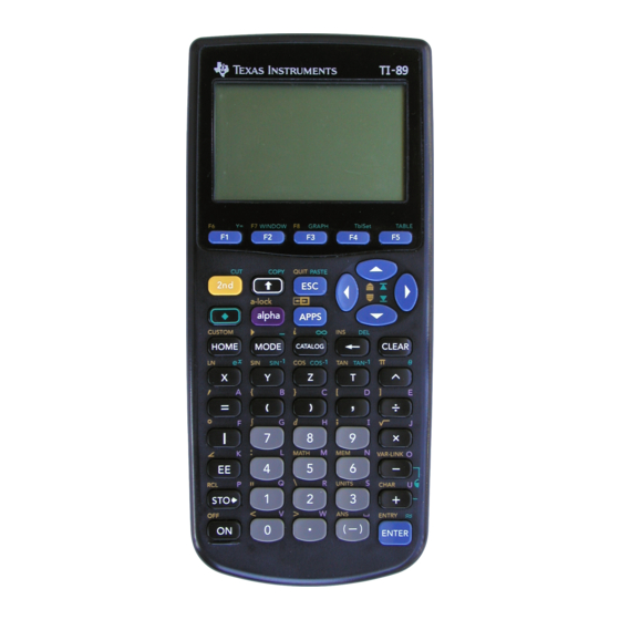
Texas Instruments TI-89 Tip List

Texas Instruments TI-89 Tip List

Graphing calculator
Hide thumbs Also See for TI-89:
Table of Contents

Advertisement

Neither I, Doug Burkett, nor any of the contributors to this tip list are responsible in any way
for any damage of any kind that you or anyone else may incur from using the information in
this tip list. These tips are provided for educational purposes only. The contributors and I
believe that all information is accurate and reliable, but we make no expressed or implied
warrantee or guarantee to that effect. Some tips may involve hardware or software
modifications to the calculator that may void the manufacturer's warrantee.
This document is a collection of useful tips and hints relating to the TI-89 and TI-92 Plus calculators.
The tips come from user experience and many other sources, and apply to all facets of calculator
operation and programming. The tip list has grown to include reference material, humor and oddities,
so perhaps the name Tip List, is no longer appropriate, but it stands for now.
The tip list is not a buglist, a wishlist or a FAQ. I maintain a wishlist, and good FAQs are available.
While a FAQ is, by definition, frequently asked questions, this list instead describes useful techniques
which may be 'infrequently asked'. These are sophisticated calculators and some features are not
obvious. All users have different skills, and what is obvious to some is not obvious to all.
I want the tip list to be the ultimate, exhaustive source of TI-89 / TI-92+ operation. If you find a good tip
or clever solution, please email me. In general I give credit to the first person to submit a particular tip.
Let me know if your tip is from a manual, or you really learned it from someone else. If a tip gives no
credit, that only means I came up with it on my own, not that I am the original inventor.
Bhuvanesh Bhatt has generously volunteered to keep this list on his site:
http://triton.towson.edu/~bbhatt1/ti/
Thanks Bhuvanesh! Bhuvanesh also maintains a bug list for these calculators.
Through the gracious efforts of Andrew Cacovean, the tip list is also available here:
http://www.angelfire.com/realm/ti_tiplist/
Andrew developed and maintains this site. You can download the entire tip list or individual tips, tip list
code and also the wishlist. Andrew has also written some very good examples of operation.
TI-89 / TI-92 Plus Tip List 10.0
Compiled by Doug Burkett, dburkett@infinet.com
Created 12 aug 99, revised 20 July 2002
Copyright 1999-2002 Doug Burkett. All rights reserved.
Dedicated to my wife,
Janet Katherine Scholz Burkett,
who cheerfully tolerates all this silliness...
Important!
0 - 1

Advertisement

Table of Contents
loading

Summary of Contents for Texas Instruments TI-89

  • Page 1 All users have different skills, and what is obvious to some is not obvious to all. I want the tip list to be the ultimate, exhaustive source of TI-89 / TI-92+ operation. If you find a good tip or clever solution, please email me. In general I give credit to the first person to submit a particular tip.
  • Page 2 Some tips include code listings, which can be typed in. Most of the code is included in a zip file called tlcode.zip. I use lots of comments and white space in these listings, so you will save considerable RAM or archive memory by deleting these comments. Beginning with version 9.0, the code listings shown in the tips are not the same as those in the tlcode.zip file.
  • Page 3: Table Of Contents

    1-19 ..... . . [1.16] Use your TI-89 / TI-92 Plus as an on-screen ruler and protractor 1-20 ..............
  • Page 4 ......[2.25] Factor on complex i to show polynomial complex coefficients 2-18 ..........[2.26] limit() fails with piecewise functions 2-18 3.0 Data structure tips...
  • Page 5 ..[5.5] Use TalkTI to develop PC applications which communicate with the TI-89 / TI-92 Plus ......
  • Page 6 ........[6.51] Review of TI-89 / TI-92 Plus Calculus Tools 6-88 .
  • Page 7 ......[9.13] Disable ALPHA default in TI-89 AMS 2.05 dialog boxes 9-17 .
  • Page 8 ......... . . [11.6] Use solve() as multiple-equation solver 11-6 .
  • Page 9: Contributors

    Contributors Contributors are credited in each tip. I would also like to list them here, and thank them again. Andrew Andy Kenneth Arnold Alex Astashyn Bhuvanesh Bhatt Billy Damien Cassou Andrew Cacovean Jordan Clifford cybernesto Martin Daveluy Stuart Dawson George Dorner Fabrizio Larry Fasnacht Glenn E.
  • Page 10: Revision Record: 9.0 To 10.0

    [D] Correct entries for avgRC(), setMode(), Table, Logistic. New tips added: [1.15] Permission to copy TI guidebooks [1.16] Use your TI-89 / TI-92 Plus as an on-screen ruler and protractor [1.17] Quick tips [1.18] Myth and legend from the TI discussion Groups [1.19]...
  • Page 11 [4.15] Delete statistics plots from programs [5.8] Opening variables in GraphLink changes some characters [5.9] GraphLink software sends either TI-89 or TI-92 Plus files [5.10] Run GraphLink under Windows XP [5.11] Improve font size of printed program source code Use R>P θ () for four-quadrant arc tangent function [6.48]...
  • Page 12: 1.0 Miscellaneous Tips

    Subject heading: ! Put something in the Subject field, it's hard to get to the post otherwise. ! Use something short but descriptive of your question/comment. Do not just put "TI-89", or "HELP!!!". ! Do not say "please read", the people likely to have an answer read all the posts anyway.
  • Page 13: [1.3] Alphabetic List Of Reserved Variable Names

    [1.3] Alphabetic list of reserved variable names The TI-89 / TI-92 Plus have several system variables and reserved names. These can be found in the manual. However, the TI-92 Plus module manual list was not updated. The most up-to-date list of...
  • Page 14: [1.4] Importing And Exporting Pc Data With The Ti-89 / Ti-92 Plus

    TI-89 / TI-92 Plus manual. That list shows the reserved names grouped by application type, and the list is not alphabetized. This makes it tedious to determine if a variable name is reserved. The table below shows all the reserved names, alphabetized. Variable names that start with greek letters are first in the table.
  • Page 15 Sending text variables to the calculator 1. Create the text in some application. 2. Use the standard Windows commands to copy the data to the clipboard. Even if the program Copy command does not explicitly mention the clipboard, the application most likely places a copy in the clipboard.
  • Page 16 The basic steps are: 1. Import the matrix data in the spreadsheet. 2. Enter the spreadsheet formulas which create an ASCII program in a spreadsheet column. 3. Cut and paste the ASCII program to a text editor, and save it as a text file. 4.
  • Page 17 In the two cells in column E following the last augment() expression, enter these two strings to create the program footer: EndPrgm \stop92\ This table shows the spreadsheet to create a 3x3 matrix. The TI-Basic program name will be makemat(), and the matrix will be called mat1. \start92\ \comment= \NAME=makemat...
  • Page 18: [1.5] Creating Picture Variables On A Pc

    While it is possible to create the picture variables directly on the TI-89 / TI-92 Plus, it is faster and easier to create them on the PC, then convert them to the calculator format. To convert them, use John Hanna's Image File Viewer program, which you can get here: http://users.bergen.org/~tejohhan/iview.html.
  • Page 19 This description assumes that you are using a PC with Windows. If you have some other operating system, the basic procedure is the same. I welcome your comments on the procedure for other operating systems. Pictures are displayed in the Graph window. The general process is: 1.
  • Page 20: [1.6] Manual Error For Setmode() Codes For Angle Modes

    To use your pictures in your programs, read about these commands in the manual: RclPic, AndPic, XorPic and RplcPic. [1.6] Manual error for SetMode() codes for Angle modes The on-line PDF verson of the TI-89 / TI-92 Plus Guidebook has an error in Appendix D, page 585. The codes for Angle should be Angle...
  • Page 21: [1.8] Make A Protective Plastic 'Skin' For Your Calculator

    [1.9] Physical characteristics of TI-89 and TI-92 Plus The table below shows some physical characteristics of the TI89 and TI92+. The characteristics for the TI-89 are for a HW1 calculator. Numbers in parenthesis refer to notes following the table. 1 - 10...
  • Page 22 Overhead LCD Agency approvals FCC Part 15 FCC Part 15 Canadian Class B Canadian Class B C-TIC (Australian) C-TIC (Australian) Patent markings 3819921 (same as TI-89) 3921142 3932846 4115705 4208720 4348733 Country of manufacture Taiwan R.O.C. Taiwan R.O.C. Copyright date...
  • Page 23: [1.10] Patents For Ti-89 And Ti-92

    This section contains abstracts of the six patents listed on the calculators, and additonal patents which may apply to graphing calculators in general. All the patents are assigned to Texas Instruments. For the full patent text including claims and figures, search by patent number at the US Patent and Trademark Office, here: http://www.uspto.gov...
  • Page 24 selecting the location in the ROM for read out of the next instruction. Input and output terminals are provided for keyboard input, display output, timing signals, etc. A test mode of operation is provided for quality control upon completion of manufacture of the chip. The test mode allows the entire ROM to be tested by reading in addresses to the address register from external and reading out the resulting word from the instruction register.
  • Page 25 The following patents are not listed on the calculator, which means that they may not include claims which apply to the TI-89 and TI-92 Plus. However, it is good practice to mark the product with all relevant patents, because this aids in proving willful infringement during litigation, with its attendant treble damages.
  • Page 26 5,168,294 Display demonstration system for providing enlarged projected image of calculator display [magnifying device for View Screen] Inventor(s): Davis; Peter H.; Christensen; Brad V.; Ahlfinger; Robert R. Issued/Filed Dates: September 27, 1991 / December 1, 1992 A calculator or other computing device uses a remote display set upon an elevated platform above the base of an overhead projector.
  • Page 27: [1.11] "Low Battery" Indication Voltages

    There are two levels of low-battery indication. The first level at the highest battery voltage is displayed as "BATT". The second level at a lower voltage is displayed as "BATT" in inverse video (white characters on a black background). This table shows the battery voltages for a HW1 TI-89 and a HW2 TI-92+.
  • Page 28: [1.13] Developer's Guide Describes Calculator Internal Operation

    [1.13] Developer's guide describes calculator internal operation The SDK developer's guide, formally called the TI-89 / TI-92+ Developer Guide, is a 1400-page document which describes much of the internal operation of the calculator. While this document is intended to enable software developers to write calculator applications, it is interesting reading even if you have no intention of writing applications, but you are just curious as to how your calculator works.
  • Page 29 5. Let the calculator dry for at least 24 hours. 6. Reassemble the calculator. See instructions below. The instructions below apply to a HW1 TI-89 and a HW2 TI-92+. They may not apply to other hardware versions. Disassembly and assembly instructions for the TI-89 You will need a small Phillips screwdriver (#0), a Torx T6 driver, and a small flat-blade screwdriver to pry out back-up battery.
  • Page 30: [1.15] Permission To Copy Ti Guidebooks

    Permission to Copy TI Guidebooks and Teacher Guides Texas Instruments (TI) grants you permission to copy and distribute, but not modify, all or any portion of any user support documents on this web site (http://www.education.ti.com). You can use this material for the purpose of preparing classroom instructional materials and educational articles for publication.
  • Page 31: [1.16] Use Your Ti-89/Ti-92 Plus As An On-Screen Ruler And Protractor

    Use or distribution for any other purpose is expressly prohibited without written permission from Texas Instruments. Permission to use TI materials for other purposes To obtain written permission from TI to use or distribute TI materials for purposes other than those described above, contact:...
  • Page 32 Push [O] to move the origin, then push [O] again to move the target. Repeat as necessary. Push [-] on the TI-89, don't use [alpha]. [UP] Move cursor up one pixel...
  • Page 33 This feature is accomplished with the copyto_h() utility, which must be installed in a folder named util\. One version of ruler() runs on both the TI-89 and the TI-92 Plus. This table shows the measurement limits for the two calculators.
  • Page 34 Instead, I test for the unmodified key code for that letter key. For example, the [O] key is the same as the [-] key, so I just test for the [-] key code (45), instead of the [O] key code (79). The TI-89 user presses the [-] key to perform the origin/target toggle function.
  • Page 35 the cursor key moves one pixel, and pressing [2ND] with the cursor key moves the cursor a larger step. There are a few dedicated function keys, and they are not necessarily obvious, so I include a 'help' screen, which is shown each time the program starts. ruler() has two shortcomings which could be remedied.
  • Page 36 Define draw_all()=Prgm PxlHorz main\±oy PxlVert main\±ox PxlHorz main\±ty PxlVert main\±tx PxlCrcl main\±oy,main\±ox,2 EndPrgm © help() © Display help dialog box Define help()=Prgm Dialog Title "Ruler Help" Text "[O] Set origin" Text "[M] Measure" Text "[STO▶] Copy measurement to Home" Text "[H] Help" Text "To quit:"...
  • Page 37 © set [H] key code 8273→khm © set [HOME] key code .013772→main\±scl © set scale factor in inches/pixel else 159→main\±x © For TI-89: set maximum x-dimension 77→main\±y © set maximum y-dimension 45→ko © set [O] key code 53→km © set [M] key code 56→kh...
  • Page 38 move_y(mode,⁻1) © Move cursor 1 pixel up draw_all() © Update screen ElseIf key=344 Then © [DOWN] move_y(mode,1) © Move cursor 1 pixel down draw_all() © Update screen ElseIf key=4436 Then © [2ND] [RIGHT] move_x(mode,10) © Move cursor 10 pixels right draw_all() ©...
  • Page 39: [1.17] Quick Tips

    13. The STAT VARS screen (ShowStat command) shows sample standard deviation, not population deviations. Display the population standard deviation by entering σx or σy. To enter the σ character, use [DIAMOND] [ ( ] [alpha] [S] on the TI-89, or [2ND] [G] [S] on the TI-92 Plus. ·(·(f(x,y),y),x) 14.
  • Page 40: [1.18] Myth And Legend From The Ti Discussion Groups

    [1.18] Myth and legend from the TI Discussion Groups "The duty of Old Timers: Since there is no known archive of these discussion groups, there ought to be a written history." - oark "Alright, you asked for it. Just keep in mind that early written histories spent generations as oral histories before someone wrote them down, and thus they became exaggerated,...
  • Page 41 And so Kremer will be lost to a history untold." This doesn't sound very good for you Ray. I advise you to cheat fate and defend the TI-89 and TI-92 Plus lest these things befall you. However, you do seem to be a central figure after the Troll War.
  • Page 42 all must serve. And one day he spoke the runes and cast the bones, and the lightening lit the night skies, and the thunder rolled without end, and Ray of Kremer cried "Behold! From the void, I have created the new land of OffTopic for you, my brothers and sisters. Rejoice and be glad, but bloody well behave yourselves this time!"...
  • Page 43 calculated, and not a machine. And emperor Kilby was short with them, and said unto them, 'no, you twits! a machine which calculates!' And the minions did say 'oh, OK, gotcha', and they did go forth and toil, and toiled some more, until there came forth the beast with the eight baleful red eyes, and it was named the DataMath 2500, but the ways of the marketing witches are strange and without reason.
  • Page 44 But the empire of TI did not slumber, and the minions toiled, and toiled some more, and little by little built a leviathan after their own hearts. And the name of this leviathan was 92, with eye bigger than 48SX, and brain faster than 48SX, and memory deeper than 48SX, and knowledge broader than 48SX. And thus it came to pass that 92 was a worthy adversary to 48SX, and begat his progeny 89, who was much the same but could ride in a really big pocket instead of a small chipcart.
  • Page 45 Thereafter most of the battles took place there, and the land of 89 and 92+ was saved from the horrors of war. And through the end of the Golden Age, and even a bit after it ended, the jihad carried on in the battlefield of comparisons, and the warriors fought each other valiantly on the fields were the bones of many fallen heros lay.
  • Page 46 Not very long after this, the creators decided that the road they had built to lead apprentices to their temple was dull, and they feared that many apprentices would lose interest along the way. So they sent the malevolent and omnipotent goddess tispt, who is known to some by another name, to rebuild the road.
  • Page 47 Legends of the discussion groups: "The Platter of Amusements" by Ray Kremer [2:56, 12/27/01] In the olden days there were three great cities of amusements. There was the city of Tee Aye Fyles, but the years took their toll on that city and it fell into ruins, and eventually even the rubble where it had stood could not be found.
  • Page 48 delight much in directing the apprentices to go to the library and read the scroll which held the knowledge they did seek. Over the years, the library grew much, and it eventually held many times the scrolls that it had begun with. And the other sages of the Realm did praise the Library of Fak and the great sage Ray Kremer who had built it and filled it with scrolls.
  • Page 49: [1.19] Kraftwerk's Pocket Calculator Song

    I have to include a bit about this song, because it may be the only one ever written about calculators. It certainly isn't specifically about the TI-89/92+, or even about graphing calculators in general. It's just a little calculator oddity.
  • Page 50 I am adding and subtracting I'm controlling and composing I'm the operator with my pocket calculator I'm the operator with my pocket calculator I am adding and subtracting I'm controlling and composing By pressing down a special key, it plays a little melody By pressing down a special key, it plays a little melody I'm the operator with my pocket calculator I'm the operator with my pocket calculator...
  • Page 51: [1.20] Ti-92 Plus Internal Photographs

    [1.20] TI-92 Plus internal photographs These photographs show the internal assembly of a TI-92 Plus, hardware version 2. Inside the back cover Component side of PCB with shield 1 - 40...
  • Page 52 Component side of PCB GraphLink I/O connector detail 1 - 41...
  • Page 53 LCD connector detail PCB, switch side 1 - 42...
  • Page 54 Key pad sheet, contact side Key pad sheet, key side 1 - 43...
  • Page 55 Key cap detail 1 - 44...
  • Page 56: [1.21] Ti-89 Internal Photographs

    [1.21] TI-89 internal photographs In case you're curious, the photographs in this tip show a disassembled TI-89, hardware version 1. Back cover with batteries and battery covers removed Back cover removed Inside view of back cover 1 - 45...
  • Page 57 Component side of PCB with shield removed A detail view of the intergrated circuits 1 - 46...
  • Page 58 Detail view of the GraphLink I/O connector PCB, switch contact side Case front cover with keypad rubber sheet in place 1 - 47...
  • Page 59 Keypad rubber sheet, key cap side Inside front cover showing keycaps in place Detail of a key cap 1 - 48...
  • Page 60: [1.22] Ti Calc-Con '02 Trip Reports

    (In the spring of 2002, Ray Kremer, Bhuvanesh Bhatt and I met in Indiana, just to get together. Ray started calling this "Calc-Con '02", obviously as a joke. I posted the following report to the TI-89 / TI-92 Plus discussion group).
  • Page 61 experience. After a short promotional film for the state of Indiana, we all enjoyed the main feature on animal migrations. The film ended at 6:30, at which point we returned to Fort Harrison, as my family and I had reserved a room at the Harrison House for the night.
  • Page 62: Ray Kremer Interview On Ti Student Features Page

    A TI-86 and a couple of TI GraphLink cables. What is your favorite TI product? The TI-86 of course, although the TI-89 and TI-92 Plus are nothing to shake a stick at. Within the TI community, what are you famous for? I have written a fairly comprehensive list of Frequently Asked Questions about TI's graphing calculators.
  • Page 63 What made you keep coming back? The first time I came to the Discussion Groups, I went into the TI-85 area and read a few posts just out of curiosity about what was there. They were mostly questions of course, and I discovered that I could answer most of them just by virtue of having thoroughly read the manual.
  • Page 64 GENERAL INTEREST: What are your favorite TI-related websites? The first things that come to my mind when you ask for well-done, useful TI-related sites are Doug Burkett's TI-TipList, Techno-Plaza, and ti-cas.org. I also frequent several other TI-related forums – TI-Programmers is one of the better ones. What is your favorite time of day? I'm most active at night.
  • Page 65: 2.0 Computer Algebra System (Cas) Tips

    I've noticed the same thing with other large equations. If you enter an expression on the command line, the TI-89 will automatically simplify it. If it is too complex, it goes as far as it can, and leave it in a bit simpler state, but doesn't finish it. If you only paste the partially simplified answer back into the input line, and hit [ENTER] again, it will finish the job.
  • Page 66: [2.3] Use When() For Absolute Values In Integrals

    x −1 x−2 x +1 x +1 x−1 In this form, the CAS returns the original equation. If you add domain constraints on x like this x −1 x−2 x +1 |x = y 2 and y > 0 x +1 x−1 the CAS will return true.
  • Page 67: [2.4] Use Exact Mode To Ensure Limit() Success

    evaluated, though, using when() to implement the absolute value function: x^2-1→f(x) á(when(f(x)≥0,f(x),-f(x)),x,-2,3) which eventually returns the approximate answer of 9.3333 3370 4891 4. The exact answer of 28/3 can be found by integrating x^2 - 1 over the three intervals [-2,-1], [-1,1] and [1,3], and summing the absolute values of the results.
  • Page 68: [2.7] Use When() In Integration In Ams 2.03

    ¶ x −1 dx = ln ( x ) which is also correctly returned by the CAS. This is not a concern if you are doing problems by hand, but if you are doing this type of symbolic integration in a program, it is worth checking for this condition and trapping it as an error, or using the correct solution.
  • Page 69: [2.10] Cas Square Root Simplification Limitations

    á(t^2*ℯ^(-s*t),t,0,∞) If the mode is set to Rectangular or Real, undef is returned. If we constrain the soluton for s>0, like this: á(t^2*ℯ^(-s*t),t,0,∞)|s>0 but leave the complex format set to rectangular, the 89/92+ is 'busy' for a long time, then returns the original integral.
  • Page 70: [2.11] Force Getnum() And Getdenom() To Return Correct Results With Part()

    If you write programs that manipulate symbolic expressions, you need to consider the domain of the variables. For example, for x < 0, 2 = −x 3 $ i = − ( −x ) 2 $ i If x = -1, then the first expression gives -i, and the second is i. Both expressions do not simplify to x^(3/2), because the identity (x^a)^b = x^(a*b) is not true for non-integer exponents a and b.
  • Page 71: [2.12] Testing Equivalence Of Symbolic Expressions

    returns a, and getdenom(temp) returns b. (Credit to Frank Westlake) [2.12] Testing equivalence of symbolic expressions The CAS (computer algebra system) of the 89/92+ does the best it can, but it can return expressions in unexpected forms. To test if two expressions expr1 and expr2 are equal, just try expr1 - expr2 which will return 0 if the two expressions are equivalent, or expr1 = expr2...
  • Page 72: [2.13] Try Comdenom() To Find Limits

    7. Try plotting the difference of the two functions over the range of interest. [2.13] Try comDenom() to find limits (Note: AMS 2.05 fixes the specific example in this tip, but the general idea may still be useful for other limits.
  • Page 73: [2.15] Use Change Of Variable In Limits Of When() Functions

    Also, it is possible to create these functions in the Program Editor. Start the editor to create a New function. In the New dialog box, set the Type to Function and enter a Variable name. Delete the Func and EndFunc lines. Finally, enter only these lines to define the function: :sec(x) :1/cos(x) This will result in a function that can be manipulated by the CAS.
  • Page 74: [2.17] Use A 'Clean' Or Empty Folder For Cas Operations

    x 4 −x 3 +8x 2 −6x+7 ( x−1 )( x 2 +2 ) 2 expand((x^4-x^3+8*x^2-6*x+7)/((x-z)*(x^2+x)^2)) −1 − which returns x 2 +2 ( x 2 +2 ) 2 ( x 2 +2 ) 2 x−1 [2.17] Use a 'clean' or empty folder for CAS operations Results from symbolic operations may not be correct if values are already defined for the variables in your expression.
  • Page 75: [2.19] Restrict Function Arguments To Integers

    returns q^2, which is just n, as desired. But this needs one more substitution, q^2 = n, to complete the simplification, and this does not work: (ln(t^n)/(ln(t))|t=p^2 and n=q^2)|q^2=n and in fact returns Memory error! To avoid this problem, Bhuvanesh Bhatt offers the following program: delay(xpr,constr) Func ©delay(xpr,constr) evaluates xpr and then imposes constraint...
  • Page 76: [2.20] Factor() With Respect To List Elements

    cos(2·Œ·@n0) which also returns 1. To type the "@" character, use [DIAMOND] [STO] on the 89, or [2nd] [R] on the 92+. (Credit to Hank Wu and Fabrizio) [2.20] factor() with respect to list elements You can use factor() to simplify expressions which include list elements. To simplify this expression a*d[1]+b*d[1]*d[2]+d[1]*d[2]*d[3] factor with respect to the list d, like this factor(a*d[1]+b*d[1]*d[2]+d[1]*d[2]*d[3],d)
  • Page 77: [2.22] Methods For Some Cas Functions

    [2.22] Methods for some CAS functions The descriptions below are from a file on the TI web site at ftp://ftp.ti.com/pub/graph-ti/calc-apps/info/92algorithms.txt These descriptions probably apply to the original TI-92, and may not accurately describe the latest version of the 89/92+ CAS. Even so, they may be useful as a general indication of how the functions get their results.
  • Page 78 factor() The methods include the well-known factorizations of binomials and quadratics, together with methods described by Geddes, Czapor and Labahn, Algorithms for Computer Algebra, Kluwer Academic Publishers, Boston, 1992. Laguerre's method is used for approximate polynomial factorization. (Press et. al: Numerical Recipes Cambridge University Press, 1986.) fMax() See fMin() fMin()
  • Page 79: [2.23] Try Comdenom() For Faster Partial Factoring

    [2.23] Try comDenom() for faster partial factoring It is not be obvious that comDenom() can be used for factoring, but this is mentioned in the TI-89/TI-92+ User's Guide, in the Alphabetical Listing of Operations section. As an example, consider the expression 6 $ x 5 −...
  • Page 80: [2.24] Infinity^0 Evaluates To 1

    [2.24] Infinity^0 evaluates to 1 The TI-89/TI-92+ CAS evaluate infinity to the zero power as one. In general, x^0 is 1, for x not equal to zero, however, since infinity is not a number, the usual rules of arithmetic do not necessarily apply.
  • Page 81 Warning: ∞^0 or undef^0 replaced by 1 I emailed TI Cares about this operation. Here is the response: "An infinity symbol is necessary for doing limits, and if it is allowed as an argument or result of the limit function, then something must be done when it is combined with other expressions. "What the TI-92 does in such compositions is consistent with extended analysis.
  • Page 82: [2.25] Factor On Complex I To Show Polynomial Complex Coefficients

    To which I would add this: A graduate student of Trinity Computed the square of infinity. But it gave him the fidgets To put down the digits, So he dropped math and took up divinity. - Anonymous [2.25] Factor on complex to show polynomial complex coefficients The CAS automatic simplification perturbs complex coefficients of polynomials, for example, ( a + bi ) x 2 + ( c + di ) x + e + fi...
  • Page 83: 3.0 Data Structure Tips

    3.0 Data structure tips [3.1] Using indirection and setFold() with matrix elements Suppose you have a matrix M of folder names, stored as strings, and you want to set the current folder in your program. This won't work: setFold(#M[k,l]) (won't work!) but this will: setFold(#(M[k,l])) (note extra parentheses around #M[k,l])
  • Page 84: [3.3] Delete Matrix Rows And Columns

    Once you have found the index, you can find the corresponding table x-value from x = dx ( index − 1 ) + x1 If the target x is less than the first x-value in the table, the equation returns zero. If the target x is greater than on equal to the last x-value in the table, the equation returns an index larger than the table size.
  • Page 85: [3.6] Convert True/False List To 0'S And 1'S

    While correct, this is hardly useful. In fact it will cause errors when used as an argument to programs that expect numeric matrix elements. You will get similar results for sizes of (2,1), (1,3) and (3,1). The work-around is to make sure you are in rectangular Vector mode when you create the matrix. This table summarizes the results of different Complex and Vector formats, and the resulting matrix that is created.
  • Page 86: [3.7] Replacement For Fill Instruction In Functions

    In this example list[] contains the True and False values, and list2[] contains the equivalent list of 0's and 1's. (Credit to Billy) [3.7] Replacement for Fill instruction in functions The Fill instruction is useful for building vectors and arrays of constants. However, since Fill is not a function, it cannot be used in 89/92+ functions.
  • Page 87: [3.9] Replace Matrix Rows And Columns

    columns with an equal number of rows. Since the program refers to the data variable, indirection is used (the # operator), and the data variable name is passed as a string. For example, to modify a data variabled named tdata, call datalist() like this: datalist("tdata") Note that the columns of data variables can be accessed with the column number in square brackets: #adata[1]...
  • Page 88: [3.10] Appending Is Faster Than Augment() For Adding Elements To Lists; Seq() Is Even Faster

    [3.10] Appending is faster than augment() for adding elements to lists; seq() is even faster Frank Westlake says that: When working with lists it can be much quicker to append rather than to augment new values. The append operation continues at the same rate, regardless of the size of the list, but the augment operation continues to decrease speed as the list grows in size.
  • Page 89: [3.13] Find Matrix Minor And Adjoint

    expr(M[j,k])→list [3.12] Don't use „list() „list() „list() „list() function in data editor NOTE: this bug has been fixed in AMS 2.05. The „list() function can be used as a column function definition. In the Data/Matrix Editor, you can define functions in the header to create columns of entries. Refer to the 89/92+ manual, page 248, for details.
  • Page 90 det(m)→d if d≠0 or gettype(d)="EXPR" then m^(⁻1)*d→n else rowdim(m)→k newmat(k,k)→n for i,1,k for j,1,k (⁻1)^(i+j)*det((mrowdel(mrowdel(m,i),j)))→n[j,i] endfor endfor endif return n EndFunc adjoint() uses equation [2] if the matrix is non-singular, or if the matrix is symbolic. There is no error checking, and a Dimension error occurs if the matrix is not square.
  • Page 91: [3.14] Randomize List Elements

    −7 6 −1 0 −1 which returns 1 −2 1 1 2 3 As an example of a singular matrix, find the adjoint of 0 1 2 0 0 0 with adjoint([[1,2,3][0,1,2][0,0,0]]) 0 0 1 0 0 −2 which returns 0 0 1 (Credit to Mike Roberts for pointing out equation [2]) [3.14] Randomize list elements...
  • Page 92: [3.15] Turn Pretty Print Off To Display Commas In Lists, Matrices

    variables, not local variables. 89/92+ functions cannot write to global variables, only local variables, so sorta will not work in a function. None the less, this method is sufficiently short that it can be embedded into your programs. The necessary global variable can be deleted when your program exits. (Credit to Daniel Lloyd) [3.15] Turn Pretty Print off to display commas in lists, matrices If Pretty Print is turned On, list and vector elements are separated with spaces in the history display:...
  • Page 93 1,1,1 1,1,2 1,2,1 1,2,2 2,1,1 2,1,2 2,2,1 2,2,2 For a particular element location {a }, we can find the corresponding list element index k from k = a 3 + a 2 − 1 d 3 + a 1 − 1 d 2 d 3 This can be expanded and factored to eliminate one multiply, and access each variable only once, like this: k = d 3 d 2 a 1 −...
  • Page 94 is a 3-element list that specifies the list dimensions as {d is the array list or the name of the array list m3rcl() returns a scalar result. To get the element at location {1,2,3} in a 2 x 3 x 4 array mat1, and save it in the variable var1, use m3rcl({1,2,3},{2,3,4},mat1)→var1 The index formula can be extended as needed for arrays of higher dimensions.
  • Page 95 This function shows the general expression to find the list index k for an element location {a ,...,a for an array of dimension {d ,...d mrankni(a,d) Func ©({loc},{dim}) return index ©Return list index for array element ©30nov00/dburkett@infinet.com; based on expression by Bhuvanesh Bhatt Σ(when(i≠dim(a),(a[i]-1)*‹(d[j],j,i+1,dim(d)),a[i]),i,1,dim(a)) EndFunc For example, to find the list index for the element at {1,2,3} in a 3x3x3 array, use...
  • Page 96 ©Rank 3 matrix ©25oct00 dburkett@infinet.com local a1,a2 intdiv(i-1,d[2]*d[3])+1→a1 intdiv(i-1-(a1-1)*d[2]*d[3],d[3])+1→a2 {a1,a2,i-d[3]*(d[2]*(a1-1)+a2-1)} EndFunc Find element address for a rank-4 array: m4aind(i,d) Func ©(index,{d1,d2,d3,d4}) return {a1,a2,a3,a4} ©Rank 4 matrix ©25oct00 dburkett@infinet.com local a1,a2,a3 intdiv(i-1,d[2]*d[3]*d[4])+1→a1 intdiv(i-1-(a1-1)*d[2]*d[3]*d[4],d[3]*d[4])+1→a2 intdiv(i-1-((a1-1)*d[2]*d[3]*d[4]+(a2-1)*d[3]*d[4]),d[4])+1→a3 {a1,a2,a3,i-d[4]*(d[3]*(d[2]*(a1-1)+a2-1)+a3-1)} EndFunc Find element address for array of any rank: mnaind(i,d) Func ©mnaind(i,dims) returns the array location of ith list element...
  • Page 97 EndFunc As an example, use m3aind() to find the element address of the 7th element of a 3x3x3 array: m3aind(7,{3,3,3}) returns {1,3,1} This example for m4aind() finds the 27th element of a 4x4x4x4 array: m4aind(27,{4,4,4,4}) returns {1,2,3,3} This example for mnaind() finds the address for the 40th element of a 5x4x3x2x1 array: mnaind(40,{5,4,3,2,1}) returns {2,3,2,2,1}...
  • Page 98 m1!→m3 Find the factorial of each integer element sin(m1)→m3 Find the sine of each element (also works for cos(), ln(), etc) (m1,x)→m3 Differentiate each array element with respect to x In general, more complex operations may be handled by nested for-loops that manipulate each array element.
  • Page 99 aRcl({loc},{dims},{arr}) Returns the array element at location loc for an array arr of dimensions dims aSto(val,{loc},{dims},{arr}) Returns the array arr of dimensions dims with the value val stored at location loc. To store this aSto(val,{loc},{dims},{arr})→myarray changed array, use newArray({dims}) Returns the list corresponding to an array of dimensions dims Contract({arr1},{dims1},{arr2},{dims2}) Contracts on the last index of arr1 and the first index of arr2.
  • Page 100: [3.17] Conditional Tests On Lists

    listSwap({list},i1,i2) Swaps the i1 and i2 elements of list (Credit to Bhuvanesh Bhatt for the general index and address expressions and programs, the transpos() function, and lots of help with this tip!) [3.17] Conditional tests on lists Suppose you have two lists L1 and L2 and you want to know if they are identical, that is, each element of each list matches the other.
  • Page 101: [3.19] Test A List For Identical Elements

    This is a well known way to exchange two elements. I include it only because you might be tempted, as I was, to do it in a more convoluted way. Note that this function takes advantage of the fact that you can write to the function arguments.
  • Page 102: [3.21] Convert Matrices To Single-Row Or Single-Column Vectors

    Both of these methods first convert the matrix to a list, then use min() and max() to find the most extreme element. [3.21] Convert matrices to single-row or single-column vectors It is occasionally necessary to convert a matrix to a row- or column-vector. To convert a matrix to a column vector, use this: mat2cvec(m) Func...
  • Page 103: [3.22] Create Lists With Logarithmic Element Spacing

    [3.22] Create lists with logarithmic element spacing Lists with logarithmic element spacing are useful for creating function plots with logarithmic x-axis scaling, and for making tables of functions which change rapidly for small values of the indpendent variable, but less rapidly for larger values. This program creates such a list. loglist(l,h,n) Func ©(xl,xh,n) make list of n+1 elements from xl to xh with log-spacing...
  • Page 104 than 32 flags, you can use lists of integers. This method of using a single bit for a flag has these advantages, compared to using a single true/false variable for each status item: ! Less RAM is used, if the program requires many status flags. ! Large groups of flags can be quickly initialized.
  • Page 105 Next, suppose that status is 0b00000111. To clear bit 1, use bitclr(status,1)→status then status would be 0b00000101. We may need to reverse the status of a flag, and bitnot() is used to do that. Suppose that status is 0b00000000, then bitnot(status,7)→status results in status = 0b10000000, and bit 7 has been changed from 0 to 1.
  • Page 106 We can simultaneously test several status flags by using a mask. A mask is simply an integer with certain bits set or cleared, as needed to perform some desired operation. We will use the built-in boolean operators and, or, xor and not to perform mask operations. For example, suppose we want to execute a block of code if flags 0, 4 and 7 are all set.
  • Page 107 flags and mask = {0b0110,0b1000} All the previous examples have shown the bit number argument passed as a number. It may, of course, be a variable instead, and you can improve program readability by choosing appropriate variable names for the flags. As an example, suppose that we have a program which may or may not calculate four sums, three limits and two integrals.
  • Page 108 The code for the four bit manipulation functions is shown below, and some explanation follows the listings. Code for bitset() - set a bit bitset(x,b) Func ©(wordOrList,bit#) set bit# ©18may01/dburkett@infinet.com local k,msg,type "bitset() err"→msg gettype(x)→type when(type="NUM",when(b<0 or b>31,msg,exact(x or 2^b)),when(type="LIST",when(b<0 or b>32*dim(x)-1,msg,augment(left(x,k-1),augment({exact(x[k] or 2^(b-(k-1)*32))},right(x,dim(x)-k)))|k=1+intdiv(b,32)),msg)) EndFunc...
  • Page 109: [3.24] Use Equations To Build Lists Of Lists And Matrices

    Func ©(wordOrList,bit#) test bit# ©22may01/dburkett@infinet.com local k,msg,type "bittst() err"→msg gettype(x)→type when(type="NUM",when(b<0 or b>31,msg,exact((x and 2^b)≠0)), when(type="LIST",when(b<0 or b>32*dim(x)-1,msg,exact((x[k] and 2^(b-(k-1)*32))≠0)|k=1+intdiv(b,32)),msg)) EndFunc All of the calculation for each function is performed with a single nested when() function: even though the listings above show three lines, each when() is a single TIBasic line. If the argument is a single integer, the function tests the bit number argument to ensure that it is between 0 and 31, since an integer has 31 bits.
  • Page 110: [3.25] Internal Error With Seq() And Boolean Operators In List Index Calculation

    and, interestingly, this {{1,2},{3,4}} returns the matrix However, you can create lists of lists and even more complicated data structures by using the list as an expression in an equation. Casting the first example in this form like this {3,a={1,2},b={3,4}} simply returns the list in the same form.
  • Page 111: [3.26] Find Indices Of Specific Elements In Lists And Matrices

    seq(t[1 and 0hF],k,0,1) In this example, t is the list, and the Boolean and operator is used to calculate the index. k is the sequence variable, and its limits are immaterial. Remember that Boolean operations on integers must be executed in Exact or Auto mode; in Approx mode they will fail with a Data Type error. The last example is the simplest possible command which demonstrates the error, but you would not likely attempt this, anyway.
  • Page 112 indexlst(l,v) func ©(l,v) return list of k|l[k]=v ©3nov01/dburkett@infinet.com local k,r,j {}→r ©Initialize result list ... 1→j ©... and result list index for k,1,dim(l) ©Loop to test each list element if l[k]=v then ©If list element matches target ... k→r[j] ©... save index in result list j+1→j ©...
  • Page 113 j→s[i,1] ©... save row index r[i]-n*(j-1)→s[i,2] ©... find and save column index endfor endif return s ©Return matrix of indices EndFunc The function returns an empty string ("") if the target value is not found. The calling program or function can test the result with getType() to determine if there are any matching indices.
  • Page 114 Tip [12.2] shows how to get around this by installing a couple of hacks. Note that you must use the correct version of inlist() for your calculator model: .89z for the TI-89, and .9xz for the TI-92 Plus.
  • Page 115 // throw the appropriate error if the user enters too many or // too few arguments, or doesn't enter a LIST or MATRIX if (argumentNumber > 2) ER_throwVar (940); if (argumentNumber < 2) ER_throwVar (930); if (*listPointer != LIST_TAG) ER_throwVar (90); // get a pointer to the second argument itemPointer = next_expression_index (listPointer);...
  • Page 116: [3.27] Fast Symbolic Determinants

    [3.27] Fast symbolic determinants The TI-89/92+ may take quite a while to find some symbolic determinants with det(). For example, a HW2 TI-92+ takes about 11 seconds to return the determinant of this matrix: d sin ( e ) f Timité...
  • Page 117: [3.28] Fill A List Or Matrix With A Constant

    For j,i+1,n m[j,i]→r If not is_0(r) Then r*m[i]-p*m[j]→m[j] q*⁻p→q EndIf EndFor EndFor Return 1/q*‹(m[k,k],k,1,n-3)*(m[n-2,n-2]*(m[n-1,n-1]*m[n,n]-m[n-1,n]*m[n,n-1])-m[n-2,n-1]*(m[n-1 ,n-2]*m[n,n]-m[n-1,n]*m[n,n-2])+m[n-2,n]*(m[n-1,n-2]*m[n,n-1]-m[n-1,n-1]*m[n,n-2])) EndFunc [3.28] Fill a list or matrix with a constant The built-in Fill command will fill a list or matrix with a constant expression, but it is not a function and cannot be used in TI Basic functions, nor return the result to the entry line.
  • Page 118: [3.30] Singular Value Decomposition (Svd) Of A Matrix

    local mθ,k,l,d,dl list▶mat(#mσ[1],1)→mθ © Convert first data column to matrix rowdim(mθ)→d © Find row dimension 2→k © Loop through remaining data columns loop #mσ[k]→l © Convert column to a list dim(l)→dl © Find row dimension if dl=0 then © Done when row dimension is zero exit elseif dl≠d then ©...
  • Page 119 m = u $ d $ v T u is a column-orthogonal matrix with dimensions a x b. d is an a x a diagonal matrix with positive or zero elements (these are the singular values), and v is an a x a orthogonal matrix. The call for Rivera's svd() is svd(m,"u","d","v") where m is the matrix to decompose, and "u", "d"...
  • Page 120: [3.31] Store New List Element At Index Greater Than Dimension

    dd→#é DelVar e1,uu,vv,dd EndPrgm Note that svd() creates and deletes global variables e1, uu, vv and dd; your own variables with those names, if any, will be deleted. (Credit to Hernan Rivera) [3.31] Store new list element at index greater than dimension You can store elements beyond a list's current dimension, if the new index is only one more than the dimension.
  • Page 121: 4.0 Graphing And Plotting Tips

    4.0 Graphing and plotting tips [4.1] Plot "vertical" lines on graph screen A vertical line is not a function, and the Y= Editor only plots functions, so you can't really plot a vertical line. There are at least three ways to plot a nearly vertical line as Y= function. Method 1 Definie a function like this: y1=1E100*(x-n)
  • Page 122: [4.2] Use Dispg To Force Update To „X And „ Y

    [4.2] Use DispG to force update to „ „ „ „ x and „ „ „ „ y „x and „y are system variables that represent the distance between the centers of two pixels in the graph view window. These variables are a calculated from the system variables xmin, xmax, ymin, and ymax.
  • Page 123 Local tlist,xlist,exp2 ClrDraw DispG DelVar τy1,τy2 exp1|y=τy2→exp2 exp1|y=τy1→exp1 augment(seq(expr("when("&string(exp1|x=xx)&",τy1,0)"),xx,xmin,xmax,„x*2),seq(exp r("when("&string(exp2|x=xx)&",τy2,0)"),xx,xmin+„x,xmax,„x*2))→tlist augment(seq(x,x,xmin,xmax,2*„x),seq(x,x,xmin+„x,xmax,2*„x))→xlist For τy1,ymin,ymax,„y*2 τy1+„y→τy2 PtOn xlist,tlist EndFor DelVar τy1,τy2 EndPrgm exp1 is the expression to be plotted, which must evaluate to true or false. The window variables xmin, xmax, ymin and ymax must be set before this program is called. This program will work on both the 89 and the 92+, since the program plots to view window coordinates, not absolute pixel coordinates.
  • Page 124: [4.4] Plot Data And Functions Simultaneously

    DispG DelVar τy1,τy2 exp1|y=τy2→exp2 exp1|y=τy1→exp1 augment(seq(expr("when("&string(exp1|x=xx)&",τy1,0)"),xx,xmin,xmax,„x*res),seq(e xpr("when("&string(exp2|x=xx)&",τy2,0)"),xx,xmin+„x,xmax,„x*res))→tlist augment(seq(x,x,xmin,xmax,res*„x),seq(x,x,xmin+„x,xmax,res*„x))→xlist For τy1,ymin,ymax,„y*res τy1+„y→τy2 PtOn xlist,tlist EndFor DelVar τy1,τy2 EndPrgm This varies from Andrew's original program only in that the window corner coordinates are passed as arguments, and the plot resolution can be set as a function argument as well. Specifically: exp1: Expression to be plotted xxmin, xxmax: Minimum and maximum x-coordinates...
  • Page 125 ©xyn: xy data plot number ©fplot: function to plot; expression ©fpn: function plot number local umode,gmode ©Save user's modes getmode("ALL")→umode stogdb gmode ©Set graph modes as needed setmode({"Graph","Function","Split Screen","Full"}) ©Clear previous graph contents clrgraph clrdraw fnoff plotsoff ©Get number of data points rowdim(xyspec)→xyrows ©Convert xy data points to lists mat▶list(submat(xyspec,1,1,xyrows,1))→xlist...
  • Page 126: [4.5] 3D Parametric Line And Surface Plots

    ! Display the graph screen using trace so that the data points and function can be traced. Control returns to the program after the user is done viewing the graph. Both the data points and the function can be traced, as usual, with the [UP], [DOWN], [LEFT] and [RIGHT] cursor movement keys. The user must press [ENTER] or [ESC] to continue running the program.
  • Page 127: [4.7] Graphing Piece-Wise Defined Function With A Unit Step Function

    y1 = x | x<3 y2 = -(x+3) | x3 and x<5 y3 = 1/2*x | x 5 Note that this method does not define a single, piece-wise continuous function. Instead, it defines several functions that, when plotted simultaneously, give the appearance of a single function. (Credit to Fabrizio) [4.7] Graphing piece-wise defined function with a unit step function This is another method to plot piece-wise continuous functions.
  • Page 128: [4.9] Faster Plots Of Slow Functions

    y1=f1(x) When the graph screen is displayed, both x^2 and x^3 will be plotted as separate plots. [4.9] Faster plots of slow functions The built-in 89/92+ function plotter can be very slow to plot complicated or time-consuming user-functions when the ZoomFit menu item is used. It seems that the plotter evaluates the function twice at each plot point, perhaps to determine the window limit system variables.
  • Page 129: [4.10] Faster Plots Of Integral Functions

    This program has these limitations: You can only plot a single function. The program will over-write current data plot definitions; use the pn parameter to specify which data plot to use to avoid this. For simple functions, the built-in function plotter is faster. You must pass the function name as a string, and the independent variable must be x.
  • Page 130 plotintg(fname,x0,xl,xh,pn,res) Prgm ©(f(x) or "f(x)",lower · limit,xlow,xhigh,plot#,xres) plot ·(f(x)) ©leaves global variables xx and yy ©11dec00/dburkett@infinet.com local dxx,k,p © dxx is the x-distance between the plotted points © k is a counter in the loops © p is (screen width - 2) ©Delete any existing xx and yy variables delvar xx,yy ©Find x-step and make x-list...
  • Page 131 You should run plotintg() in Approx mode, and the Graph Mode must be set to FUNCTION. This same program works with either the 89 or the 92+. If you have a global variable called x, delete it before running plotintg(). These are the program arguments: fname The name of the function to be plotted, as an expression or...
  • Page 132 A design goal for the program was never to attempt to plot beyond the maximum x-value specified by xh. This goal is desirable because the function might not even be defined beyond xh, or it might be increasing so rapidly that the resulting y-axis scaling would degrade the plot resolution. This is prevented by using the floor() function to calculate the number of points plotted.
  • Page 133 getmode("0")→umode ©Set modes to Function plot, full screen, and Approx setmode({"1","1","8","1","14","3"}) ©Initialize settings if nonexistent ©The settings are saved as global variables, for defaults each time the program ©is executed. If igrand does not exist, the program assumes none of the ©parameters exist, and they are initialized to valid values.
  • Page 134 title et text "Lower plot limit" text "must be less than" text "upper plot limit" enddlog goto l1 ©Validate plot resolution elseif res≤0 or fpart(res)≠0 then dialog title et text "Resolution must be an" text "integer greater than zero" enddlog goto l1 ©Validate data plot number elseif dpn≤0 or dpn>99 or fpart(dpn)≠0 then...
  • Page 135: [4.11] 3D Data Plots

    igrand, lil, lpl, upl, res, dpn Finally, if you're curious as to what the sine integral looks like over the range of zero to 15: [4.11] 3D data plots The 89/92+ can plot 3D functions in a few ways, but they cannot plot 3D data, that is, a set of discrete points in three dimensions.
  • Page 136: [4.12] Random Scatter Plots Of 'Noisy' Functions

    [4.12] Random scatter plots of 'noisy' functions The function plot feature of the TI-89/92+ will plot, at most, one point for each x-axis display pixel. If the function is rapidly changing, the resulting graph will not accurately represent the function. For example, the Y= editor was used to make this graph, with a resolution of one: The graph shows the error for a Chebychev polynomial fit of ln(x) for x=1 to x=2.
  • Page 137 This program, scatterf(), draws this type of scatter plot. scatterf(f,x,xl,xh,yl,yh,n) Prgm ©("f(var)","var",xmin,xmax,ymin,ymax,its) ©Function scatterplot with random points ©13aug01 dburkett@infinet.com local k,e false→e ©Clear graph screen clrgraph clrdraw plotsoff fnoff clrio ©Set x- & y-axis ranges xl→xmin xh→xmax yl→ymin yh→ymax ©Loop to plot the function points for k,1,n if getkey()≠0:exit (xh-xl)*rand()+xl→xn...
  • Page 138: [4.13] Bode Plots

    A sample call would be scatterf("y1(x)","x",1,2,¯3,4,1000) which plots 1000 points of the function y4(x) from x=1 to x=2, with a y-axis range of -3 to 4. scatterf() plots each point as it is calculated, so you can see the plot develop. You may stop scatterf() by pressing any key.
  • Page 139 = jw j = −1 where (Electrical engineers use j for the complex unit, but the TI-89/92+ use i). In the frequency domain, we work with frequencies in radians/second, not Hz, so first we convert the frequencies of interest: 10 Hz = 62.83 rad/sec...
  • Page 140 To create the list of sequential integers, use seq(k,k,1,51)→xcoord Note that the number of elements, 51, is one more than the loglist() argument of 50, since loglist() returns one more element than the number specified. Now that we have the three lists, it is a simple matter to use the built-in data plotting functions to create the plots.
  • Page 141 For both the magnitude and phase plots, you can use [F3] to trace the graph and read either the magnitude or the phase at the bottom of the display, as the yc variable. However, you cannot directly read the frequency, since the xc variable only shows the elements of the xcoord list. You can, though, manually display the frequency.
  • Page 142: [4.14] Completely Clear Graph Screen

    developing a comprehensive regenerative feedback theory. He invented techniques for synthesizing networks with desired characteristics, which has applications in telephone line equalization. He also worked with R. B. Blackman and Claude Shannon to model messages and signals in probabilistic terms, which was a new idea at the time. Hendrik Bode is obviously not the other well-know Bode, the German astronomer Johann Elert Bode, who lived from 1747 to 1826.
  • Page 143: 5.0 Graphlink Cable And Software Tips

    5.0 GraphLink Cable and Software Tips [5.1] Unarchive variables to fix GraphLink transmission errors This tip applies to GraphLink software for Windows 95/98, beta version, and the gray and black cables. It may also apply to other operating systems and GraphLink software versions. If you try to send a variable to the calculator, and that variable is locked, you will get a transmission error.
  • Page 144: [5.4] Try Var-Link To Fix Graphlink Transmission Errors

    To be completely safe, use the procedure in tip [5.2] to transfer your data and programs from your HW1 calculator to the HW2 calculator. In general this means transferring programs and variables individually with GraphLink, then restoring them individually to the HW2 calculator. (Credit to Lars Frederiksen) [5.4] Try Var-Link to fix GraphLink transmission errors Some ASM programs may crash your calculator, requiring that the batteries be removed.
  • Page 145 for 'black-compatible cable', because it is compatible with TI's black cable. The BCC works with TI's GraphLink software; other cable designs require custom third-party software. The BCC is built with inexpensive, non-critical, readily available parts. I have built both BCC versions, and they work quite well.
  • Page 146 The schematic for the original cable is shown above. The connection to the computer may be either a DB9 or a DB25 connector; the DB25 pin numbers are shown in parentheses. The GraphLink plug which connects to the calculator is a 3-conductor (stereo) 2.5 mm connector. The three conductors are named like this: 5 - 4...
  • Page 147 The parts list for the original cable: Designator Value Comments D1, D2, D3, D4 1N914 May also be 1N4148, 1N4004. Not critical. Q1, Q2 2N4401 May also be 2N3904, or any NPN transistor with at least 25V collector-emitter voltage rating Q3, Q4 2N3906 Any PNP transistor with at least 25V...
  • Page 148 The parts list for the deluxe cable: Designator Value Comments D1, D2, D3, D4 1N914 May also be 1N4148, 1N4004. Not critical. Q1, Q2, Q5, Q8 2N4401 May also be 2N3904, or any NPN transistor with at least 25V collector-emitter voltage rating Q3, Q4, Q6, Q7 2N3906 Any PNP transistor with at least 25V...
  • Page 149 RadioShack parts list for BCC deluxe Designator Value RadioShack part number Total cost US$ D1, D2, D3, D4 1N914/1N4148 276-1122 (pack of 10) 1.19 Q1, Q2, Q5, Q8 2N4401 276-2058 1.96 Q3, Q4, Q6, Q7 PN2907 276-2023 2.36 R1, R2, R3, R4 100kohm, 1/8W, 10% 276-1347 (pack of 5) 0.49...
  • Page 150 Components are shown in black, jumper wires in red, and off-board connections are blue. Note that the PCB is not vertically symmetrical; the two rows of single pads are near the top. This layout shows the component side of the board. All components are mounted on this side, but it will be easier to mount some of the jumpers on the reverse side (called the solder side).
  • Page 151 10. Check your work for solder bridges, which are particularly likely with RadioShack PCBs, because the pads and holes are so large. 11. Test the cable. Circuit description The GraphLink cable has three conductors. Two of the conductors are data lines, which connect to the tip and the ring of the 2.5mm plug.
  • Page 152 cases 1 and 2, the calculator is either in the idle state, or the 'other' data line is asserted low, so the plug tip and CTS must follow the RTS line state. The BCC circuit implements these cases as follows. Case 1: RTS is at about +12V relative to serial port ground.
  • Page 153 The voltage source V may be a power supply or even a 9V battery. The two resistor Ra and Rb set voltage Vh, and simulate the 10K source impedance of the calculator data lines. For a desired source impedance Rs and output voltage Vh, use these equations to find Ra and Rb: Rs$V Rs$V Ra =...
  • Page 154 3. You have selected the correct serial port for your computer. 4. You have reasonably fresh batteries in the calculator. 5. Both the GraphLink and serial port connections are secure. On the TI-89, in particular, the GraphLink cable connector must be firmly pushed into the calculator connector.
  • Page 155: [5.7] Graphlink Switchbox Aids Cbr/Cbl Programming

    programs using the SEND button in the GraphLink windows. This can usually be fixed by executing Recieve or Get Screen from the GraphLink menu. If you use the GraphLink software to develop CBL or CBR programs, you may want to build the switch-box circuit (described in tip [5.7] below) into your BCC.
  • Page 156 ! char(13) pastes as the carriage return symbol in TI Basic programs on the calculator, but pastes as an actual carriage return in GraphLink. For the character codes, refer to the table TI-89 / TI-92 Plus Character Codes in Appendix B of the TI-89/TI-92+ Guidebook.
  • Page 157: [5.9] Graphlink Software Sends Either Ti-89 Or Ti-92 Plus Files

    2. In the List Files of Type drop-down menu, choose All Files (*.*), then choose the desired file. 3. In the File Name text box, type *.89* to list all TI-89 files, or type *.9x* to list all TI-92 Plus files.
  • Page 158: [5.10] Run Graphlink Under Windows Xp

    Note also that most other GraphLink operations work with either calculator; for example, the screen grab and calculator backup and restore functions work correctly, regardless of which calculator is actually connected. [5.10] Run GraphLink under Windows XP Various visitors to TI's discussion groups have shared their tips on getting the Graph Link and TI Connect software running under Windows XP.
  • Page 159: 6.0 Math Tips

    Converting from a very complicated rectangular form to polar form in the exact or auto mode, can be extraneous on our TI-89 operating systems. Internal complex calculations are done in rectangular form. So, the polar complex numbers are converted to rectangular form.
  • Page 160: [6.3] Improving Floating-Point Solutions To Simultaneous Equations

    (103.416 < 27.1821) is generated in about 1 second. [6.3] Improving floating-point solutions to simultaneous equations Round-off errors in matrix calculations can create errors larger than you might expect when finding solutions to simultaneous equations with simult(). The closer the matrix is to being singular, the worse the error becomes.
  • Page 161 As an example, consider using simulti() to find the coefficients for the Langrangian interpolating polynomial. This is just the polynomial that fits through the given points. A polynomial of degree n-1 can be fit through n points. This function returns the coefficients as a list, given the x-y point coordinates in a matrix: polyfiti(xyd) func...
  • Page 162 gamma(z) Func © Γ(Z) by Stirling's formula ©M.Dave1 If real(floor(z))=z:Return when(z>0,(z-1)!,undef) Local n,x,y when(real(z)<0,1-z,z)→x 10-min(floor(abs(x)),10)→n n≠0:x+n→x approx(ℯ^(⁻x)*x^(x-0.5)*√(2*Œ)*polyEval({0.00083949872087209,⁻5.1717909082606⁻005,⁻0.000 59216643735369,6.9728137583659⁻005,0.00078403922172007,⁻0.0002294720936214,⁻0.0026813271 604938,0.0034722222222222,0.083333333333333,1},1/x)*when(n=0,1,‹(1/(x-k),k,1,n)))→y approx(when(real(z)<0,Œ/(sin(z*when(sin(Œ)=0,Œ,180)))/y,y)) EndFunc This function works for all real and complex arguments. The accuracy is near full machine precision, except for very large negative arguments. Since the gamma function is similar to the factorial function, the result overflows the calculator floating point range for relatively small arguments.
  • Page 163: [6.5] Round Numbers To Significant Digits

    [6.5] Round numbers to significant digits You may need to round a number to a specified number of significant digits. For example, this can be useful when simulating arithmetic on a different processor with fewer significant digits, or estimating the effects of round-off error on function evaluation.
  • Page 164: [6.6] Linear Regression Through A Fixed Point

    [6.6] Linear regression through a fixed point It can be useful or necessary to force a regression equation through a fixed point. For example, you might be modelling a system, and you know from the physical laws that the function must pass through (0,0).
  • Page 165: [6.7] Complex Derivatives

    which returns {1.3483146067416,0} This data can be used to test the routine for a fit through an arbitrary point: xl = {100,200,300,400,500} yl = {140,230,310,400,480} h = 300 k = 310 which returns {0.85, 55} This function can be used to find the unadjusted correlation coefficient for the curve fits: corrhk(f1,xl,yl) func ©(f1,xlist,ylist)return r^2 for y=f1(x)
  • Page 166: [6.8] Convert Trigonometric Expressions To Exponential Format

    − a 2 +b 2 2$a$b ( a 2 +b 2 ) 2 ( a 2 +b 2 ) 2 If you fail to specify the variables as complex, you may not get the answer you expect. For example, the derivative of the complex conjugate function conj() is undefined, yet (conj(z),z)|z=a+bi returns 1, which is not correct for complex z.
  • Page 167: [6.9] Convert Floating-Point Numbers To Exact Fractions

    Setting constraints on a and b may result in a more simple expression. (Credit to Glenn Fisher) [6.9] Convert floating-point numbers to exact fractions The usual method to convert a floating-point number n to an exact fraction is to use exact(n). However, this function will only work for numbers smaller that the 14-digit precision of the 89/92+.
  • Page 168 Func ©~cubic(p,v) Roots of cubic equ p - cubic equ v - independent var Local p,r,q,ù,a,b,u,v,w getType(é)≠"EXPR":Return "p\cubic:arg must be a cubic eq" p\coef(é,ý)→ù dim(ù)≠4:Return "p\cubic:arg must be a cubic eq" string(cZeros(é,ý))→w inString(w,".")=0 and w≠"{}":Return expr(w) ù[2]/(ù[1])→p ù[3]/(ù[1])→q ù[4]/(ù[1])→r (3*q-p^2)/3→a (2*p^3-9*p*q+27*r)/27→b (√(3*(4*a^3+27*b^2))-9*b)^(1/3)*2^(2/3)/(2*3^(2/3))→w If getType(w)="NUM"...
  • Page 169 Exit EndIf EndFor ú[k]→y √(ù[2]^2/4-ù[3]+y)→r If r=0 Then √(3*ù[2]^2/4-2*ù[3]+2*√(y^2-4*ù[5]))→d √(3*ù[2]^2/4-2*ù[3]-2*√(y^2-4*ù[5]))→e Else √(3*ù[2]^2/4-r^2-2*ù[3]+(4*ù[2]*ù[3]-8*ù[4]-ù[2]^3)/(4*r))→d √(3*ù[2]^2/4-r^2-2*ù[3]-(4*ù[2]*ù[3]-8*ù[4]-ù[2]^3)/(4*r))→e EndIf {⁻ù[2]/4+r/2+d/2,⁻ù[2]/4+r/2-d/2,⁻ù[2]/4-r/2+e/2,⁻ù[2]/4-r/2-e/2} EndFunc coef(): coef(è,ý) Func ©~coef(p,v) Make list of coefficents p - polynomial v - independent var Local ù,é,ì getType(ý)≠"VAR":Return "p\coef:2nd arg must be a VAR" If inString(string(è),"=")>0 Then left(è)→é...
  • Page 170 EndIf Else augment(o,{l[i]})→o EndIf EndFor If f=0 Then Else EndIf EndFunc cubic() is used to solve cubic (third-order) equations, and quartic() solves 4th-order equations. coef() and evalrt() are used by cubic() and quartic() to find the solutions. evalrt() can also be used on the results from cubic() and quartic(), as described below, to expand the solutions.
  • Page 171 ✍ = ✬ + 1 3$✬ ✎ = ✬ − 1 3$✬ ( −3$ ( 69 −9 )) 3 $2 3 $3 6 $2 ( 9− 69 ) ✬ = The first three elements are the solutions to the cubic polynomial. The last three elements define the variable substitutions used in the solutions.
  • Page 172: [6.11] Rounding Floating Point Numbers

    If you call cubic like this: cubic(x*(x-3)*(x+2)-7*(x-3)*(x+2)*i,x) then the returned solutions are {-2,3}: the complex solution of 7i is not returned. However, if cubic() is properly called with the underscore, to indicate that x is complex, like this cubic(x_*(x_-3)*(x_+2)-7*(x_-3)*(x_+2)*i,x_) then the correct solutions of {-2, 3, 7i} are returned. cubic() and quartic() first try to find an exact solution with czeros().
  • Page 173 The basic method is to replace nsolve() with a TI Basic program that uses Newton's method, coupled with an accurate estimating function. Further speed improvements are possible since you control the accuracy of the solution. The function is called fipoly(), and here is the code: fipoly(clist,fguess,yval,yemax,yetype) func ©Fast inverse polynomial solver...
  • Page 174 The function parameters are clist List of coefficients for the polynomial that is to be solved. fguess List of coefficients of the estimating (guess) polynomial yval The point at which to solve for x yemax The maximum desired y-error at the solution for x, must be >0 yetype A string that specifies whether yemax is absolute error or relative error: "abs"...
  • Page 175: [6.13] Find Coefficients Of Determination For All Regression Equations

    s = 5493.68334077 t = -2422.15013853 u = 425.883370029 So, to find x when y = 1.5, with a relative error of 1E-8, the function call looks like this: fipoly(fclist,fglist,1.5,1E-8,"rel") which returns x = 2.6627... Using the same test cases as in tip [11.5], the table below shows the execution times and errors in x for various maximum y error limits, for both the relative and absolute error conditions.
  • Page 176 Endfunc r2coefdf(lx,ly) func ©Find coefficient of determination r^2, adjusted for DOF ©lx is list of x-data points ©ly is list of y-data points ©24 nov 99/dburkett@infinet.com local n dim(lx)→n 1-((n-1)*sum((regeq(lx)-ly)^2))/((n-dim(regcoef)-1)*sum((ly-mean(ly))^2)) Endfunc Note that neither of these functions will account for weighting of the data points. Both functions should be run in Approx mode.
  • Page 177: [6.14] Use Norm() To Find Root Mean Square (Rms) Statistic For Matrices

    where m is the number of coefficients in the equation. For the simple linear equation y = ax + b, m = 2, because we have two coefficients a and b. It is appropriate to use r without DOF adjustment when the data to be fit has no experimental errors. For example, this is the case if you are fitting a curve to data generated by some other mathematical function.
  • Page 178: [6.16] Transpose Operator And Dot Product Find Adjoint And Complex Scalar Product

    These programs use built-in conversion functions to perform these general coordinate transformations on the equation: x = r $ cos(✕) y = r $ sin(✕) r = ! x 2 + y 2 ✕ = tan −1 The transformation equations might not return the results you expect, because the last two equations ✕...
  • Page 179: [6.17] Use Dd.mmssss Format To Convert Angles Faster

    [6.17] Use dd.mmssss format to convert angles faster Surveyors and civil engineers commonly measure angles in degrees, minutes, seconds and fractions of a second. The 89/92+ can convert these angles to decimal angles: just enter the angle on the command line, and enter it: 12°34'56"...
  • Page 180: [6.18] Use Ipart() And Int() Effectively

    ©By Doug Burkett & anonymous poster ©Angle a1 is returned in format dd.mmsss, 12.345678 = 12°34'56.78" ©Assumes angle 'a1' is degrees if angle mode is Degree, or radians if the mode is Radian. if getmode("angle")="RADIAN":a1*57.295779513082→a1 ipart(a1)+.01*(ipart(60*fpart(a1)))+.006*fpart(60*fpart(a1)) Endfunc In summary: dms() converts an angle in DMS format to degrees in Degree mode, or radians in Radian mode. dmsi() converts an angle to DMS format.
  • Page 181: [6.20] Generating Random Numbers

    Integration limits Integral t = 1 to t = 2 0.1359 0512 1983 28 t = 2 to t = 3 0.0214 0023 3916 549 t = 3 to t = 4 0.0013 1822 6789 7969 t = 4 to t = 5 3.1384 5902 6124 E-5 t = 5 to t = 6 3.8566 4984 2341 4 E-7...
  • Page 182: [6.21] Evaluating Polynomials

    You may want to use RandSeed to reset or initialize the random sequence. Also note that the randNorm() function returns normally distributed random numbers. [6.21] Evaluating polynomials You don't need to explicitly calculate a polynomial like this: 2*x^3 + 3*x^2 + 4*x - 7 → result Instead, TI BASIC has a polyEval() function that uses less ROM space: polyEval({2,3,4,-7},x) →...
  • Page 183: [6.23] Step-By-Step Programs

    These sites have programs that solve various problems step-by-step, that is, the program shows each of the steps used to solve a problem. I have not tried these programs. Oliver Miclo's ti-cas site: http://www.ti-cas.org/ ! Compute derivative: stepder.89g (TI-89) or stepder.9XG (TI-92+) ! Solution of linear systems: invm() TIcalc site: http://www.ticalc.org/pub/89/basic/math/ ! Solve Diophant equations: diophant.zip...
  • Page 184: [6.24] Fast Fibonacci Numbers

    TIcalc site: http://www.ticalc.org/pub/92/basic/math/ ! Solve n equations in n unknowns using Gauss-Jordan elimination: srref.zip [6.24] Fast Fibonacci Numbers The Fibonacci numbers are defined by this recurrence relation: = 1, = 1, This formula can be used to find the nth Fibonacci number: 1+ 5 1−...
  • Page 185: [6.26] Accurate Numerical Derivatives With Nderiv() And Ridder's Method

    func ©Convert vector v to polar [R▶Pr(v[1,1],v[1,2]),R▶Pθ(v[1,1],v[1,2])] EndFunc rect(v) func ©Convert vector v to rectangular [P▶Rx(v[1,1],v[1,2]),P▶Ry(v[1,1],v[1,2])] EndFunc polar([1,1]) [[√(2),Œ/4]]. rect([[√(2),Œ/4]]) returns returns [1,1]. Note that these routines assume the current Angle Mode setting. If the angle mode is radians, then the angles are in radians. If you or your application expect the arguments or results to be in degrees or radians, set the proper mode.
  • Page 186 The built-in functions avgRC() and nDeriv() are fast, but they may not be accurate enough for some applications. The avgRC() function can return, at best, an accuracy on the order of e , where e the machine accuracy. Since the 89/92+ uses 14 decimal digits, e = 1E-14, so the best result we can expect is about 1E-7.
  • Page 187 ✜ nder2("tan", /2.01) which returns 16374.242. The absolute error is about 1.01E-4, and the relative error is 6.19E-9. The table below demonstrates the improvement in the derivative estimate as h decreases, for tan(x) evaluated at x = 1. f'(x) difference in f'(x) 1E-2 3.4264 6416 009 (none)
  • Page 188 (√(abs(expr(ffun)/(d3/(h1^2)))))/10→hh if hh=0: .01→hh endif ©Initialize for solution loop (expr(fphh)-expr(fmhh))/(2*hh)→amat[1,1] big→err ©Loop to estimate derivative for i,2,ntab hh/con→hh (expr(fphh)-expr(fmhh))/(2*hh)→amat[1,i] con2→fac for j,2,i (amat[j-1,i]*fac-amat[j-1,i-1])/(fac-1)→amat[j,i] con2*fac→fac max(abs(amat[j,i]-amat[j-1,i]),abs(amat[j,i]-amat[j-1,i-1]))→errt if errt≤err then errt→err amat[j,i]→dest endif endfor if abs(amat[i,i]-amat[i-1,i-1])≥safe*err:exit endfor return {dest,err} endfunc nder1() is called with the function name as a string, the evaluation point, and the initial step size. If the step size is "auto", then nder1() tries to find a good step size based on the function and evaluation point.
  • Page 189 The value h is an initial step size. It should not be too small, in fact, it should be an interval over which the function changes substantially. I discuss this more in the section below, More comments on nder1() and Ridders' method. To use nder1() and return just the derivative estimate, use nder1(f,x,h)[1] where [1] specifies the first element of the returned list.
  • Page 190 reslist[1]→nderout dialog title "NDER1 RESULTS" text "Input x: "&string(xx) text "dy/dx: "&string(reslist[1]) text "Error est: "&string(reslist[2]) text "(Derivative → nderout)" enddlog if ok=0:return goto lp EndPrgm To use nderui(), nder1() must be saved in a folder called nder. nderui() should be stored in the same folder.
  • Page 191 Input x is the point at which the derivative is estimated. dy/dx is the derivative estimate. Error est is the error estimate. The derivative estimate is saved in the global variable nderout in the current folder. Push [ENTER] to find another derivative, or press [ESC] to exit the program. Diagnosing nder1() with nder1p() nder1p() uses the same algorithm as nder1(), but is coded as a program instead of a function.
  • Page 192 if d3=0: .01→d3 (√(abs(expr(ffun)/(d3/(h1^2)))))/10→hh if hh=0: .01→hh endif clrio disp "Starting interval hh: "&string(hh) newmat(ntab,ntab)→amat (expr(fphh)-expr(fmhh))/(2*hh)→amat[1,1] big→err for i,2,ntab hh/con→hh (expr(fphh)-expr(fmhh))/(2*hh)→amat[1,i] con2→fac for j,2,i (amat[j-1,i]*fac-amat[j-1,i-1])/(fac-1)→amat[j,i] con2*fac→fac max(abs(amat[j,i]-amat[j-1,i]),abs(amat[j,i]-amat[j-1,i-1]))→errt if errt≤err then errt→err amat[j,i]→dest endif endfor if abs(amat[i,i]-amat[i-1,i-1])≥safe*err then disp "SAFE limit exit" exit endif endfor...
  • Page 193 There are other methods for finding numeric derivatives. For example, you can fit a polynomial (either Lagrange or least-squares) through some sample points, then find the derivative of the polynomial. These methods might not have any speed advantage over nder2(), because an accurate, high-order polynomial requires considerable time to find the coefficients, although it is fast to find the derivative once you have them.
  • Page 194 If we could let h=0, then this equation would return the exact derivative. However, h=0 is obviously not allowed. Further, we can't just make h arbitrarily small, because the loss of precision degrades the answer. This can be seen by using nDeriv() with various values of h. The table below shows the results returned by nDeriv() for f(x) = tan(x), with various values of h, and with x = 1 f'(x) error...
  • Page 195 tan ( x+h ) −tan ( x−h ) sin ( x+h )( cos ( x−h ) −cos ( x+h ) sin ( x−h )) 2$h$cos ( x+h ) cos ( x−h ) This is a clever trick, because it converts the tangent function, which has asymptotes, into a function of sines and cosines, which don't have asymptotes.
  • Page 196 error 0.001 3.74E-10 0.005 1.48E-10 0.01 2.22E-11 4.70E-12 0.15 2.00E-12 1.64E-11 -1.10E-12 -4.60E-12 4.93E-01 Note that the error suddenly increases at hh = 0.5. Obviously, there is a best value for hh that reduces the error, but this best value is not too sensitive to the actual value of hh, as the error is on the order of E-12 from hh = 0.1 to 0.4.
  • Page 197: [6.27] Find Bernoulli Numbers And Polynomials

    abs ( f ( x )) f ∏∏ ( x ) where I have used the absolute value abs() to ensure that the root is real. I also divide the final result by 10 to ensure that h is small enough that nder1() doesn't terminate too early. nder1() can terminate in one of two ways: if the error keeps decreasing, nder1() will run until the amat[] matrix is filled with values.
  • Page 198 or, as mentioned above, by evaluating B (0). However, a faster method to find Bernoulli numbers on the 89/92+ uses this identity: ( −1 ) n−1 B 2n ( 2✜ ) 2n ✛ ( 2n ) = 2 ( 2n ) ! ✛...
  • Page 199 ¶ ff2 = ff1 − ff1 ( x ) dx To find the nth Bernoulli polynomial requires finding all the (n-1) previous polynomials, so this is time-consuming for higher-order polynomials. For this reason I wrote two different versions of programs to find the Bernoulli polynomials. One version is a function which returns a single polynomial of the order specified by the function argument.
  • Page 200 ©1jul00/dburkett@infinet.com ©Save polynomials in list bpoly[]. local k,k1,k2,bpdim,ff1,usermode,choice ©Save user's mode; set modes getmode("all")→usermode setmode({"Complex Format","Real","Vector Format","Rectangular","Exact/Approx","Exact","Pretty Print","Off"}) ©If bpoly[] exists unarchive it, else create it & initialize it. if gettype(spfn\bpoly)="NONE" then newlist(1)→spfn\bpoly x-1/2→spfn\bpoly[1] else unarchiv(spfn\bpoly) endif dim(spfn\bpoly)→bpdim clrio ©Loop to derive Bernoulli polynomials if nxx>bpdim then augment(spfn\bpoly,newlist(nxx-bpdim))→spfn\bpoly for k,bpdim+1,nxx...
  • Page 201 Endfunc These routines must both be installed in a folder called \spfn. The list of Bernoulli polynomials will be created in this same folder. To create a list of polynomials, execute bnpoly(n) where n is the highest-order polynomial you expect to use. For example, if you use polynomials up to the 20th order, then use bnpoly(20).
  • Page 202: [6.28] Bilinear Interpolation

    However, it turns out that the 89/92+ are extremely slow to find the dimension of lists with large elements, even if the lists have few elements. For example, if the bpoly[] has 70 polynomials, its size is dim(spfn\bpoly) about 24000 bytes, and takes over 30 seconds to return the dimension of 70! If dim(bpoly) bpoly[] has 100 elements,...
  • Page 203 Bilinear interpolation If we are given four (x,y) points such that ) = z > x ) = z > y ) = z ) = z then we can solve for a function in four unknown coefficients. There are an infinite number of such equations, but the most simple candidate is z = ax + bx + cxy + d so the system to solve for a, b, c and d is...
  • Page 204 (y-ya)/(yb-ya)→u (1-t)*(1-u)*zaa+t*(1-u)*zba+t*u*zbb+(1-t)*u*zab EndFunc Note that the variable names have been changed to avoid conflict with built-in variables. The equivalence is xa == x ya == y zaa == z zab == z xb == x yb == y zba == z zbb == z The z-variables are named so it is easy to remember which z-variable goes with a particular (x,y) data point.
  • Page 205 request "y1",ya request "y2",yb request "f(x1,y1)",zaa request "f(x1,y2)",zab request "f(x2,y1)",zba request "f(x2,y2)",zbb enddlog expr(xa)→xa expr(xb)→xb expr(ya)→ya expr(yb)→yb expr(zaa)→zaa expr(zab)→zab expr(zba)→zba expr(zbb)→zbb if ok=0:return string(x)→x string(y)→y dialog title "bilinui" request "x",x request "y",y enddlog expr(x)→x expr(y)→y if ok=0:return bilinint(xa,xb,ya,yb,zaa,zab,zba,zbb,x,y)→z dialog title "bilinui result" text "z= "&string(z) enddlog if ok=0:return...
  • Page 206 This method is good enough for many problems, assuming that the function changes slowly, and the x- and y-values are close enough together such that the function is 'close' to linear in both variables. The interpolated values change smoothly and gradually within a particular x and y pair, but the derivatives change abruptly as you move to the next row or column of the original data table.
  • Page 207 z 9 = a $ x 3 2$ y 3 2 + b $ x 3 2 $ y 3 + c $ x 3 $ y 3 2 + d $ x 3 2 + e $ y 3 2 + f $ x 3 $ y 3 + g $ x 3 + h $ y 3 + j In matrix form this system is written as x 1 2 $ y 1 2 x 1 2 $ y 1 x 1 $ y 1 2 x 1 2 y 1 2 x 1 y 1 x 1 y 1 1 x 1 2 $ y 2 2 x 1 2 $ y 2 x 1 $ y 2 2 x 1 2 y 2 2 x 1 y 2 x 1 y 2 1...
  • Page 208 and the inverse is 1 − 1 2 4 − 4 − 4 − − 3 4 1 − 1 4 1 − 1 4 2 −2 2 − − 3 − 3 1 − 1 − 1 1 −2 0 −1 X −1 = −1...
  • Page 209 Three-element list of the table x-coordinates {x1,x2,x3} Three-element list of the table y-coordinates {y1,y2,y3} zmat 3x3 matrix of the table z-values The x-value at which to interpolate The y-value at which to interpolate The z-values are passed as a 3x3 matrix only because that is a convenient way for the user to enter the z-values, directly as they appear in a printed table.
  • Page 210 title "INPUT ERROR" text "Entry error for" text msg text "Push ENTER to try again" enddlog EndPrgm ©Create lists & matrix newlist(3)→xl newlist(3)→yl newmat(3,3)→zmat ©Initialize variables "0,0,0"→x123 "0,0,0"→y123 "0,0,0"→zz1 "0,0,0"→zz2 "0,0,0"→zz3 "0,0"→xy 1→inhome Lbl in1 ©Prompt for input variables dialog title "INTRP9UI"...
  • Page 211 res[3]→yl[3] endif ©Extract row 1 z-variables util\rq3v(zz1)→res if res="ERR" then errdisp("z row 1") if ok=0 then return else goto in1 endif else res[1]→zmat[1,1] res[2]→zmat[1,2] res[3]→zmat[1,3] endif ©Extract row 2 z-variables util\rq3v(zz2)→res if res="ERR" then errdisp("z row 2") if ok=0 then return else goto in1...
  • Page 212 ©Do the interpolation math\intrpz9(xl,yl,zmat,x,y)→z ©Display result dialog title "RESULT" text "x: "&string(x) text "y: "&string(y) text "" text "z = "&string(z) text "" dropdown "Put z in Home?",{"no","yes"},inhome text "" text "Push ENTER to interpolate again" enddlog ©Copy result to home screen if inhome=2 util\copyto_h(string(x)&","&string(y),z) ©Exit, or interpolate again...
  • Page 213: [6.29] Dirac's Delta (Impulse) And Heaviside (Step) Functions

    You can press [ENTER] to return to the input screen and do another interpolation, or press [ESC] to quit the program and return to the home screen. For each interpolation, you can copy the interpolation result to the home screen by selecting YES in the drop-down menu labelled Put z in Home?.
  • Page 214: [6.30] Spherical Coordinate Conventions

      0 for x < 0 H ( x ) =   1 for x > 0   This is defined as a function with Define H(x)=when(x<0,0,when(x=0,undef,1)) Sometimes the Heaviside function is defined as   0 for x < 0 ...
  • Page 215: [6.31] Fast 2Nd-Order Interpolation With Quadreg

    [6.31] Fast 2nd-order interpolation with QuadReg Linear interpolation is adequate for most table-interpolation problems. A second-order (quadratic) interpolation is more accurate, but it does require entering one more data point. The first-order (linear) interpolation uses two points to find the coefficients a and b in ax + b = y then calculates y at your desired x.
  • Page 216 Prgm ©2nd-order interpolation ©15oct00 dburkett@infinet.com ©calls str2var() local a1,b1,a2,b2,a3,b3,x1y1,x2y2,x3y3,x © Initialize all the point variables © (note that a1==x1, b1==y1, etc) 1→a1 2→b1 3→a2 4→b2 5→a3 6→b3 0→x © Transfer control here to repeat interpolations lbl t1 © Convert x- and y-data to pairs as strings; also convert 'x' to string string(a1)&","&string(b1)→x1y1 string(a2)&","&string(b2)→x2y2 string(a3)&","&string(b3)→x3y3...
  • Page 217 © Do the regression and calculate y = f(x) quadreg l1,l2 regeq(x)→res © Display the result dialog title "QUADINT RESULT" text "x = "&string(x) text "y = "&string(res) text "y saved in 'res'" text "(Push ESC to quit)" enddlog if ok=0:goto exit1 ©...
  • Page 218: [6.32] Accurate Approximate Solutions To Quadratic Equations With Large Coefficients

    You can use this method with any of the built-in regression commands. You need to enter as many points as there are coefficients in the equation. For example, the CubicReg command fits the data to a cubic polynomial with four coefficients, so you would need to enter four points. I mentioned that the function str2var() is called by quadint().
  • Page 219: Sine And Cosine Integrals

    To put either of the roots in the history display, use a list index of [1] or [2] as needed: {0.5,0.25}[1] puts 0.5 in the history display {0.5,0.25}[2] puts 0.25 in the history display The TI92 operation mode should be set to APPROXIMATE, since the purpose of quadrtic() is to reduce floating-point arithmetic errors.
  • Page 220 These symmetry relations hold: Si ( −z ) = − Si ( z ) Ci ( −z ) = Ci ( z ) − i✜ 0 < arg ( z ) < ✜ where where ✏ = 0.577215664901533 (Euler’s constant) x d ∞...
  • Page 221 x 8 +a 1 x 6 +a 2 x 4 +a 3 x 2 +a 4 f ( x ) = 1 x + ✒ ( x ) ✒ ( x ) < 5 $ 10 −7 x 8 +b 1 x 6 +b 2 x 4 +b 3 x 2 +b 4 = 38.027264 = 40.021433 = 265.187033...
  • Page 222: [6.34] Error Function For Real Arguments

    if x=0:return 0 if x<0:return ⁻spfn\si(⁻x) if x>Œ then Œ/2-(((polyeval({1,0,38.027264,0,265.187033,0,335.677320,0,38.102495},x))/(polye val({1,0,40.021433,0,322.624911,0,570.23628,0,157.105423},x)))/(x)*cos(x)+(polye val({1,0,42.242855,0,302.757865,0,352.018498,0,21.821899},x)/polyeval({1,0,48.19 6927,0,482.485984,0,1114.978885,0,449.690326},x))/(x^2)*sin(x)) elseif x>.01 then nint(sin(z)/z,z,0,x) else polyeval({⁻2.2774643986765⁻9,0,3.0619243582207⁻7,0,⁻2.8344671201814⁻5,0,1.666 6666666667⁻3,0,⁻.055555555555556,0,1,0},x) endif EndFunc Code listing for ci(x): ci(x) Func ©(x) return ci(x), x real, |x|<112 ©Must be in folder \spfn ©23jan01/dburkett@infinet.com if x=0:return undef if x<0:return spfn\ci(⁻x)+*Œ...
  • Page 223 e −t ¶ erf ( x ) = 2 ✜ For x > -3 and x < 3, the error function looks like this: erf(x) approaches 1 and -1 for large x and large -x, respectively. Also note that erf(-x) = -erf(x). The complimentary error function erfc(x) is defined as erfc(x) = 1 - erfc(x) This function calculates erf(x) for all real x.
  • Page 224: [6.35] Cumulative Normal Distribution And Inverse

    While the function may look complicated, it is really nothing more than a series of nested when() functions to select the appropriate estimating method for value the input x argument. erf() calls itself for x<0; there is only one level of recursion. These references have more discussion of the error function: Handbook of Mathematical Functions, Abramowitz and Stegun, Dover, 1965.
  • Page 225 p ( x ) = This can be combined with [2] to yield a simple function to find the general CND, like this: cnd(x,m,s) func ©(x,m,s) find cum norm dist at x, mean m, std dev s ©Find cumulative distribution at x, with mean m and standard deviation s ©dburkett@infinet.com 8jun00 (erf(((x-m)/s)/1.4142135623731)+1)/2 Endfunc...
  • Page 226 shown here is more accurate than that included in the SLE application. For the upper-tail distribution with x = 2, mean = 0 and standard deviation = 2,the SLE returns a result of .022750062014, which is in error by about 8E-8. It is occasionally necessary to find the inverse of distribution function, that is, to find the value of the random variable x, given a probability, a mean and a standard deviation.
  • Page 227 sgn(x) = when(x≠0,sign(x),1) The function shown below, cndif(), implements the algorithm just described to find the inverse of the cumulative distribution function. cndif(p,m,s) func ©(probability,mean,std dev) inverse CND ©Inverse cumulative normal distribution ©Returns x with probability that X≤x ©Fast version. ©29oct00/dburkett@infinet.com local r,t p→r...
  • Page 228: [6.36] Integration May Return 'Undef' For Identical Integration Limits

    [6.36] Integration may return 'undef' for identical integration limits By definition, ¶ f(x)dx = 0 for any a and f(x). The TI-89/92+ evaluate such 'zero-width' integrals correctly with either nInt() or á(), unless f(x) cannot be evaluated at a. For example, these functions all return zero: á(1,x,0,0) nInt(1,x,0,0) á(x,x,0,0)
  • Page 229: [6.37] Random Number Generator Algorithm

    For some simulations and Monte Carlo numerical methods, it is important that the random number generator have a sufficiently long period. I emailed TI-cares concerning this. Here is the response: The TI-89 and TI-92 Plus all use the same random number generator. Rand() creates random numbers between 0 and 1.
  • Page 230: [6.40] Write Functions With Multiple Input Argument Types

    parcurve(f,x,y) Func ©ParCurve(f,x,y) parametrizes curve f(x,y)=0 as x(t),y(t) ©Bhuvanesh Bhatt expr("solve("&string(f=y-t*x)&" and y-t*x=0,{"&string(x)&","&string(y)&"})") EndFunc For example, to find a parametric expression for x 3 + x 2 − y 2 = 0 use the call parcurve(x^3+x^2-y^2,x,y) which returns x = t 2 − 1 and y = t 2 − 1 $ t or x = 0 and y = 0 The first two equations are the useful parameterizations;...
  • Page 231: [6.41] Integration Error In Ams 2.05

    rowdim(xx)→xxr coldim(xx)→xxc newmat(xxr,xxc)→r for j,1,xxr for k,1,xxc f1(xx[j,k])→r[j,k] endfor endfor return r else return "f1demo: type error" endif EndFunc This function accepts arguments that may be expressions, numbers, lists or matrices. If the argument is a list or matrix, the function is applied to each element. The function to be evaluated is defined as a local function f1();...
  • Page 232 ( 2x−3 ) ( 2x−3 ) 7 but the correct result is However, if symbolic values are used for the constants, the correct result is returned, that is 2 +1 2 ( ax+b ) ¶ ( ax + b ) n dx returns a ( n+2 ) If Approx mode is used instead of Auto mode, examples [1] to [3] return correct results.
  • Page 233: [6.42] Stddev() And Variance() Find Sample (Not Population) Statistics

    (called σx) after using OneVar, you must manually recall σx as follows: TI-89: [DIAMOND] [ ( ] [alpha] [S] [x] [ENTER] TI-92+: [2ND] [G] [S] [x] [ENTER] The stdDev() and variance() functions of the 89/92+ return the sample statistics, not the population statistics.
  • Page 234 ✤ 2 = s 2 n−1 ✤ = s n−1 The last line shows the identities we want, in which the desired population variance and standard deviation are functions of the sample variance and standard deviation. If desired, these definitions can be coded as simple functions: Population standard deviation: stddevp(x) Func...
  • Page 235: [6.43] Dot Product (Scalar Product) For Complex Vectors

    In these last two functions, the number of data points is found by summing the elements of the frequency list. [6.43] Dot product (scalar product) for complex vectors The built-in dotp() function can be used to find the scalar dot product for two complex vectors, but its behavior may be puzzling.
  • Page 236: [6.44] Nest Min() In Max() To Limit An Argument

    [6.44] Nest min() in max() to limit an argument You can limit an argument to two bounds upper and lower, with this expression: max(lower,min(x,upper)) For example, suppose we have a calculation in which we calculate the real inverse sine (arcsine) of the result of a previous calculation.
  • Page 237: [6.46] Solve() And Nsolve() Ignore Constraints With Local Variables

    return abs((at-(tArea(px,py,bx,by,cx,cy)+tArea(ax,ay,px,py,cx,cy)+tArea(ax,ay,bx,by,px, py)))/at)≤tol EndFunc The function returns true if point (px,py) is within the triangle defined by the points (ax,ay), (bx,by) and (cx,cy), otherwise it returns false. tol is a small positive number which specifies the tolerance at which the two areas will be considered equal. If you are using Exact mode, you may set tol = 0. If you are using the function in Approx mode, with floating point coordinate arguments, set tol to specify the precision at which you want to consider the two areas equal.
  • Page 238 In July 2001, David Dannenmiller posted an nsolve() example to the 89/92+ discussion group, where the constraints were ignored and nsolve() returned a root outside of the solution bounds. It turns out that David found a particular constraint expression which causes nsolve() to return a solution which is a root, but is outside of the solution bounds.
  • Page 239: [6.47] Unsigned Infinity Displays As Undef

    solve() shows the same behavior as nsolve(), except that it takes much longer to return the incorrect roots, and the correct root is often included as one of multiple solutions. [6.47] Unsigned infinity displays as undef 'Unsigned infinity' is sometimes used in math textbooks to indicate a limit which is +∞ on one side of the evaluation point, and -∞...
  • Page 240: [6.49] Taylor() Polynomial Function Finds Tangent Line

    Neither of these results are useful. A more elaborate function can be written which also handles list and matrix arguments: atan2(αx,αy) Func ©(x,y) 4-quadrant arctan(y/x) ©Must be installed in math\ ©6jan02/dburkett@infinet.com local αt,εm,τx © Function name, error message, αx type "atan2 error"→εm ©...
  • Page 241: [6.50] The Savage Benchmark

    m = d f ( x ) x x = a then n = b − m $ a and if f(a) = b, we find n with The tangent line is the first-order Taylor series polynomial at x = a, so we can use the built-in taylor() function to find the line equation.
  • Page 242 benchmark n. [techspeak] An inaccurate measure of computer performance. "In the computer industry, there are three kinds of lies: lies, damn lies, and benchmarks." Well-known ones include Whetstone, Dhrystone, Rhealstone (see h), the Gabriel LISP benchmarks (see gabriel), the SPECmark suite, and LINPACK. See also machoflops, MIPS, smoke and mirrors.
  • Page 243 ! We cannot conclude that the HP-48GX is, in general, faster at numeric computation, because we have only tested a tiny subset of all the functions. ! We cannot conclude that the TI-89 / TI-92 Plus is, in general, more accurate, because again, only a tiny subset of the functions has been tested.
  • Page 244 For the TI-89 / TI-92 Plus TI Basic programs, this distinction is significant because the loop overhead is significant: 46 seconds for the TI-89 HW1, and 31 seconds for the TI-92 Plus HW2. This amounts to about 18 mS/iteration for the TI-89, and 12 mS/iteration for the TI-92 Plus.
  • Page 245 There has been some confusion about the number of significant digits used by the TI-89 / TI-92 Plus, which can be cleared up by referring to the TI SDK manual. In usual calculator operation, 12 significant digits are displayed, except for regression results, in which 14 significant digits can be shown. 14 significant digits are used for 'normal' calculator operation, and for TI Basic calculations.
  • Page 246: [6.51] Review Of Ti-89 / Ti-92 Plus Calculus Tools

    Sky & Telescope magazine, March 1987 Neither of these references discuss the benchmark in much detail. [6.51] Review of TI-89 / TI-92 Plus Calculus Tools (This review was written by George C. Dorner, September, 2001) This is a nice little package of programs for these two TI calculators. The package is downloadable for either calculator (which must be using the latest version of the calculator operating system, V.
  • Page 247 The package is a collection of programs which will be useful to students and teachers, mostly in calculus classes or courses where calculus is used. Once the package is loaded, the programs and functions basically become part of the calculator firmware. Here are the programs (functions) and a comment about each: Tangent Line and Normal Line: These two functions compute the equations of the respective lines, given a function and a value of the...
  • Page 248: [6.52] Return Complex Results In Real Mode With 0I

    The gamma function is included here, too. Its presence may encourage exploration of this complicated topic during the second calculus course and will be an occasional aid to students in applied courses. Its accuracy seems to be good beyond 5D, plenty for beginners. “Automatic”...
  • Page 249: [6.53] Implicit Derivatives

    I will skip the details here, and focus on finding implicit derivatives with the TI-89/TI-92+. The most straight-forward method to find the implicit derivative of f(x,y) is to specify y = y(x) in the expression and use the built-in differentiation function ().
  • Page 250: [6.54] Delete Variables After Using Numeric Solver

    i,2,ñ © Loop to find higher-order derivatives (e,x)+e1*(e,y)→e EndFor © Return derivative. © (Replace with factor(e) to automatically factor result.) EndFunc The arguments are impdifn(expression, independent variable, dependent variable, order) expression may be an algebraic expression, or an equation. order is the order of the derivative: 1 for the first derivative, 2 for the second and so on.
  • Page 251: [6.55] Algorithms For Factor() And Isprime()

    2, 2, 4, 2, 4, 2, 4, 6, 2, 6 to generate these primes plus a few extra harmless composites. "TI-92 Plus and TI-89 start the same way, except that they stop this trial division after trial divisor 1021, then switch to a relatively fast Monte-Carlo test that determines whether the number is certainly composite or is almost certainly prime.
  • Page 252: [6.56] Fourth-Order Splice Joins Two Functions

    "If the number is identified as composite, the factor() function then proceeds to the Pollard Rho factorization algorithm. It is arguably the fastest algorithm for when the second largest prime factor has less than about 10 digits. There are faster algorithms for when this factor has more digits, but all known algorithms take expected time that grows exponentially with the number of digits.
  • Page 253 s(x) is the splice function s ( x ) = a $ x 4 + b $ x 3 + c $ x 2 + d $ x + e In general, the splice function is s ∏ ( x ) = 4 $ a $ x 3 + 3 $ b $ x 2 + 2 $ c $ x + d and the first derivative is is the point between x and x...
  • Page 254 The c vector in [15] is the scaled coefficients; but we want the un-scaled result y = s(x). This is found with equation [9] where x−x 2 x s = [17] so s(x) can be calculated with the TI-89/92+ polyEval() function: 6 - 96...
  • Page 255 polyEval({a,b,c,d,e},k*(x-x2)) Do not expand the splice polynomial with the relationship shown in [17]! While this may seem to simplify the polynomial, it undoes the benefit of scaling, and the resulting polynomial is again unstable. Ultimately we use a single function for f(x), which is implemented as a nested when() function: when(x<x1,f1(x),when(x<x3,s(x),f2(x))) or, in terms of the splice evaluation when(x<x1,f1(x),when(x<x3,polyEval({a,b,c,d,e},k*(x-x2)),f2(x)))
  • Page 256 © © | y_1 (y1 = f1(x1)) © | y_2 (y2) © c = M^(-1) * | y_3 (y3) = f2(x3)) © | yp1 (scaled value of f1'(x1)) © | yp3 (scaled value of f2'(x3)) © © © M^(-1) has been pre-computed. The following expression is all one line. mat▶list([⁻.5,1,⁻.5,⁻.25,.25;.25,0,⁻.25,.25,.25;1,⁻2,1,.25,⁻.25;⁻.75,0,.75,⁻.25,⁻.25;0,1, 0,0,0]*[y_1;y_2;y_3;yp1;yp3]) EndFunc...
  • Page 257 For this example the difference plot crosses the x-axis, so the functions intersect at this point. We choose this point as the splice center, so that the splice will not have to span a large distance between the two functions. Solving for the root gives x 2 = 0.549220479094 In some cases, the two functions will not intersect at all, or at least in the desired splice range.
  • Page 258 (y1(x),x)-(y6(x),x)|x=x2-h returns 3.7629E-8 (y2(x),x)-(y6(x),x)|x=x2+h returns 7.446E-9 The errors seem small enough, but calculating the derivatives correctly (as shown below) gives the true errors: (y1(x0),x0)-k*(polyEval(spl4,x),x)|x=-1 and x0=x2-h returns -6.087E-11 (y2(x0),x0)-k*(polyEval(spl4,x),x)|x=1 and x0=x2+h returns 3.601E-11 So far, the splice seems to work well. As a final check, we graph the splice function over the splice interval.
  • Page 259 Note that the splice slopes still match the functions at the interval endpoints, but now the splice is above both functions. Differentiating the splice To differentiate the splice, do not expand the splice polynomial and differentiate it: accuracy will suffer because of round-off error.
  • Page 260 when(o=2,k^2*polyeval({12*a,6*b,2*c},xs), when(o=3,k^3*(24*a*xs+6*b),when(o=4,k^4*24*a,0))))) EndFunc spli4de() returns the string "spli4de err" if the order o is less than 1. No testing is done to ensure the order is an integer. Note that derivatives with order greater than four are zero. You should not, in general, use the splice function to estimate derivatives of order greater than the first, even though spli4de() provides that capability.
  • Page 261 spli4in() does not check xa and xb to ensure that they are within splice interval. Results may be inaccurate when integrating beyond the interval limits. Solving for the splice inverse Some applications require finding x such that s(x)=y, given y. This can only be done if the splice is strictly monotonic on the splice interval, that is, the splice s(x) has no minimum or maximum on the interval.
  • Page 262 We now have all the arguments for splice4(). To find x given s(x), use polyeval(spl4y,ky*(s(x)-yy2)) where ky = 1/hy. This inverse polynomial is not the true inverse of the original splice. It is simply a polynomial which passes through the same three points as the splice, and has the same derivatives at the endpoints. If the splice is used for a narrow interval, the accuracy can be very good.
  • Page 263 © yy1 f1(x1) © yy2 the mean of yy1 and yy3 © yy3 f2(x3) © hy y-interval half-width © expr("define f1(x)="&f1) © Define local functions to be spliced expr("define f2(x)="&f2) x2-h→x1 © Find splice interval bounds x2+h→x3 f1(x1)→yy1 © Find si(x1), si(x3) f2(x3)→yy3 (yy1+yy3)/2→yy2 ©...
  • Page 264 © Calls math\splice4() © Local variables local l,m,errx1,errx2,errx3,errd1,errd3,x1,äx2,x3,äh,yy1,äyy2,yy3,k,äf1,äf2,yp1,yp2,splc,äout © l drop-down selection variable © m drop-down selection variable © äf1 f1(x) © äf2 f2(x) © x1 lower interval bound © äx2 interval midpoint © x3 upper interval bound © yy1 f1(x1) ©...
  • Page 265 äf1(x1)→yy1 © Find splice bound y's äf2(x3)→yy3 if m=1 then © Set yy2 for s(x2) method: (yy1+äf1(äx2)+yy3)/3→äyy2 © ... 'mean' method elseif m=2 then (äf1(äx2)+äf2(äx2))/2→äyy2 © ... 'center' method endif (äf1(ä),ä)|ä=x1→yp1 © Find derivatives at interval bounds (äf2(ä),ä)|ä=x3→yp3 math\splice4(yy1,äyy2,yy3,äh*yp1,äh*yp3)→splc © Find splice coefficients splc→#(spl4v[6]) ©...
  • Page 266 For f1(x) and f2(x), I can just enter y1(x) and y2(x), since I have previously defined these functions in the Y= Editor. I set the splice center and half-width, and chose 'center' for the s(x2) method. I need not enter a value for 'manual s(x2)', since I am not using the manual method. After pressing [ENTER], the errors are shown on the program I/O screen: spli4ui() supports three options to set s(x2): center, mean and manual.
  • Page 267 y s −s x s −q substitute these expressions in the function definition x s −q y s = r $ f and solve for y x s −q dy s = r $ d then take the derivative dx s dx s dy s = r p $ d...
  • Page 268: [6.57] Sum Binary "1" Digits In An Integer

    ∞ ✟ I = lim s ( x ) $ ✁x m [2B] nd∞ x sb −x sa ✁x s m = where [3B] x b −x a ✁x m = [4B] Solve [3B] for n, replace in [4B], and define a new variable c such that x b −x a ✁x m ✁x s m =...
  • Page 269: [6.58] Extract Floating-Point Mantissa And Exponent

    -2,147,483,648 to 2,147,483,647. This is 0h0 to 0hFFFF. (Recall that the TI-89/TI-92 Plus use 0b to prefix binary integers, and 0h to prefix base-16 integers). sum1s() uses a table lookup (in the list t) to find the number of 1's in each 4-bit nibble of the input integer n.
  • Page 270: [6.59] Accelerate Series Convergence

    format(n,"s")→s expr(right(s,dim(s)-instring(s,"")))→e return {n*(10^⁻e),e} EndFunc If the list returned by mantexp() is stored to foo, then use foo[1] to get the mantissa, and foo[2] to get the exponent. Some examples: mantexp(0) returns {0,0} mantexp(1) returns {1,0} mantexp(100) returns {1,2} mantexp(1.23E17) returns {1.23,17} mantexp(-456E-100)
  • Page 271 s[n]→s0 © Save the individual sums we need s[n-1]→s1 s[n-2]→s2 s[n-3]→s3 s0-(s0-s1)^2/(s0-2*s1+s2)→sb © Find the last sum s1-(s1-s2)^2/(s1-2*s2+s3)→sa © Find the next-to-last sum return {sb,sb-sa} © Return the last sum, and the difference EndFunc aitkend2() is called with a list of series terms, and returns the last accelerated sum, and the difference between the last two sums.
  • Page 272: [6.60] Faster, More Accurate Exponential Integrals

    −x The TI-89 / TI-92 Plus also cannot find accurate values for this integral, and it is no wonder, since at the integrand singularity at x = 0, the limit is +infinity from the right and -infinity from the left. One...
  • Page 273 endif EndFunc I ported this algorithm, from Numerical Recipes in Fortran, to TI Basic. The input argument must be greater than zero, and error message strings may be returned. You can check for this condition by using getType() on the result. This table shows some results for the original example problem.
  • Page 274: [6.61] Find More Accurate Polynomial Roots

    [6.61] Find more accurate polynomial roots solve() may return false solutions to ill-conditioned polynomials. An ill-conditioned polynomial is one in which small changes in the coefficients cause large changes in the roots. Since zeros() uses solve(), zeros() can return the same incorrect solutions. This tip gives an example, shows how to check the results and gives alternative methods for finding the better solutions.
  • Page 275 These values may not seem 'close' to zero, still, they may be the best roots as defined above. The first step is to test each root. Command-line and TI Basic calculations on the TI-89 / TI-92 Plus are performed with a 14-digit mantissa, so we need to find the value of e for each root. If a root is expressed in scientific notation as a.bEc, where a.b is the mantissa, a is not equal to 0 and c is the...
  • Page 276 This call tests the roots returned by solve(): proot_t1({1,4.217E17,-3.981E20,-6.494E22},{-4.217E17,-141.81969643465,0}) which returns {true,true,false}, indicating that the first two roots pass the sign test and the last root fails. Note the proot_t1() also tests for f(x) = 0 for each root, and returns true in that case. proot_t1() can only be used to test real roots of polynomials with real coefficients.
  • Page 277 z2 = -4.2169 9999 9999 9 E17 (1.68E38, 3.72E39) z3 = 1085.8557 4101 61 (-5E10, 4.9E10) where the numbers in parentheses are y1(x-e) and y1(x+e). This method returns the correct first and third roots, but the second root fails the sign test. If you save your polynomials in coefficient list form and evaluate them with polyEval(), it is easy to use the list reversal method in tip [3.4] to reverse the coefficients.
  • Page 278 ©Set Complex format to Rectangular ©12may02/dburkett@infinet.com local m,roots,eps,maxm,i,j,jj,ad,x,b,c,root ©------------------------------------------------------------ © Define local function to find 1 root with Laguerre'e method Define root(a,x)=Func ©({coeffs},guess) polynomial root ©NOTE: {a} is reversed! local m,maxit,mr,mt,epss,iter,j,abx,abp,abm,err,frac,dx,x1,b,d,f,g,h,sq,gp,gm,g2 dim(a)-1→m © Find order of polynomial 2⁻12→epss © Set estimated fractional error 8→mr ©...
  • Page 279 1⁻12→eps © Set complex part limit newlist(m)→roots © Create list to hold roots seq(a[i],i,dim(a),1,⁻1)→a © reverse coefficients for simpler looping a→ad © Copy coefficients for deflation for j,m,1,⁻1 © Loop to find each root 0→x © Set guess to zero to find smallest remaining root root(ad,x)→x ©...
  • Page 280 getType(r)="STR" polyroot() uses Laguerre's algorithm for both the initial root-finding and the polishing, however, this is not mandatory: you could use some other method for the polishing. The references at the end of this tip discuss this more and give some suggestions. Since polyroot() uses complex arithmetic even to find the real roots, we have a dilemma I have not encountered before: when do we decide that a complex root is actually real, and only has a small complex part because of round-off error? It may be that the root really does have a small complex part,...
  • Page 281 reasonable to use instead. It assumes that any small imaginary part cannot be determined with an accuracy better than eps relative to the real part. In the meantime, I had tested polyroot() with about 30 polynomials from textbooks and numerical methods books, and in all cases it returned both real and complex roots, as appropriate.
  • Page 282 15504x 5 + 4845x 4 + 1140x 3 + 190x 2 + 20x + 1 Obviously, there are 20 repeated roots of -1, but proots() returns (approximately) these roots in about 100 seconds: -1.49339 ± 0.102038i -0.848193 ± 0.295003i -1.40133 ± 0.280223i -0.843498 ±...
  • Page 283 This situation is somewhat puzzling considering that the TI-86 returns, very quickly, three correct solutions. The TI-89 / TI-92 Plus probably use a more general algorithm, while the TI-86 uses an algorithm specifically designed for polynomials.
  • Page 284 References Polynomial root-finding is an important, well-developed topic in numerical analysis, so most books on numerical methods or numerical analysis include a section on finding polynomial roots. Those that have been most helpful to me follow. Numerical Recipes in FORTRAN; The Art of Scientific Computing Press, Teukolsky, Vetterling and Flannery, 1992, Cambridge University Press.
  • Page 285: [6.62] Try Asymptotic Expansion For Functions Of Large Arguments

    The present example shows that asymptotic expansion can fix a severe round-off error problem. In June 2002, a post on the TI-89 / TI-92 Plus discussion group reported problems evaluating this function for large arguments: f ( x ) = 1 −...
  • Page 286 The function starts getting erratic at about 370, and really gets chaotic at about x = 530. Since the limit of f(x) is one, there are definite problems in evaluating the function. As the problem occurs for large x, an asymptotic expansion is a potential solution. An asymptotic expansion is a series of the form a 0 + + ...
  • Page 287 a5 = − 4 6364 a 4 = 0 a 6 = 0 a 7 = − 1010625 a 9 = − 275708 a 11 = − 20793692 a 8 = 0 a 10 = 0 65690625 6897515625 a 13 = − −1335915116 a 12 = 0 a 14 = 0 596288828125...
  • Page 288: [6.63] Faster Numerical Matrix Inverses

    The plot shows the difference between the two function on the interval x = [5, 100]. The cursor readout shows that we could use x = 60 as the transition point between the functions. The function value at this point is about 0.989999885775, and the difference between the functions is about 6.3E-6. If we only need 5 or 6 significant digits in this range, the approximation is good enough.
  • Page 289: [6.64] Calculate Through Undef And Get Correct Results

    [6.64] Calculate through undef and get correct results In some cases you can calculate with undef values and still get the correct result. Suppose we want to find the reciprocal of the sum of reciprocals of numeric list elements, like this: 1/sum(1/list) where list is the list of elements.
  • Page 290: 7.0 Ti Basic Programming Tips

    7.0 TI Basic Programming Tips [7.1] Create evaluated Y= Editor equations in programs You can create equations in the 89/92+ by storing the expression to the system variables yn(x), where 'n' is the number of the equation. For example, a*x^2+b*x+c→y1(x) stores the expression to the first equation, y1(x).
  • Page 291: [7.3] Using Language Localization

    linreghk(xl,yl,h,k) func ©(xlist,ylist,h,k) return {b,a} for y=b*x+a through (h,k) When this program is selected in CATALOG, the status line shows ©(xlist,ylist,h,k) return {b,a} for y=b*x+a through (h,k) Consider using this feature to give the user all the critical documentation needed to use the function: 1.
  • Page 292 GetMode("1") True→V2XX Else False→V2XX ClrErr EndTry The V2XX variable will contain True if language localisation is supported, or False otherwise. It is convenient if the V2XX variable is a global variable, so that it can be used by functions to test for the version.
  • Page 293: [7.4] Return Error Codes As Strings

    To test for a mode in a function is a little complicated. It is necessary for an installation program to get the language dependent mode names and store them in global variable, which can be used by the functions. An example of translating Radian to the active language: If V2XX Then "3"→MAngle SetMode(MAngle,"1")→OldMode...
  • Page 294: [7.5] Considerations For Referencing External Programs

    This method fails if the function is designed to return a string instead of a number. In that case you may be able to use special coded strings for the error message. For example, suppose we have a routine that is supposed to build a string from two arguments: stringit(a,b) func if dim(a)=0 or dim(b)=0 then...
  • Page 295: [7.6] Recursion Limits

    In many cases, the problem can be avoided by just keeping a copy of B() in the same folder as A(), and using method 1 above. This approach has these disadvantages: ! If B() is used my many programs, in many different folders, RAM or archive is wasted with each copy that is necessary.
  • Page 296 stop endprgm Archive stopit(), then, at the command line, enter expr("stopit()") [ENTER] The BUSY annunciator in the LCD turns on and does not turn off. Keys seem to be recognized, but not handled. For example, pressing [green diamond] will toggle the 'diamond' annunciator, and pressing [2nd] will toggle the '2nd' annunciator.
  • Page 297: [7.8] Return Program Results To Home Screen

    4. Call the 'exit' routine as usual, but use return instead of stop to terminate program operation. [7.8] Return program results to home screen A TI-89/TI-92 Plus function can return a result to the command line, but a program usually cannot. However, there are two methods to get around this limitation.
  • Page 298 The first call to copyto_h() has only one argument (1.224), so that argument is placed in both the entry and answer columns of the history area. The next two calls have two arguments, so the first argument (the strings) is placed in the entry column, and the second argument is placed in the answer column. The last call shows that expressions are pretty-printed, as expected.
  • Page 299: [7.9] Passing Optional Parameters To Functions And Programs

    lres is a list of strings to return to the history area. You can use the "@" character to add labels to the results. Note that the input string lres is stored to the global variable wstr, so that you can also recall wstr to get the results.
  • Page 300: [7.10] Calling Built-In Applications From Your Programs

    ! You don't want to put the burden of remembering all this on the user, so it's easier to obligate the user to use the fixed number of arguments. On the other hand, Frank Westlake notes these advantages: ! You can write one function instead of several very similar functions, which saves memory. ! The user doesn't have to remember which function to use for a given case.
  • Page 301: [7.12] Access A Variable From Any Folder With "_" (Underscore)

    Func © ©Programmed copyright by Tip DS ©This program is free for use, provided ©no modification is made. There may be no ©charge for this program, unless ©permission is given in righting by ©Tip DS. For more information, right ©to tipds@yahoo.com ©...
  • Page 302: [7.13] Write To Program & Function Arguments

    store functions or programs in these variables. The variable will appear in Var-Link in the folder in which it was created. You can create these variables as global variables in programs, but not functions. You cannot create them in functions. You can execute a string stored in one of these variables like this: "test2()"→_ttt1 expr(_ttt1)
  • Page 303: [7.14] Determine Calculator Model And Rom Version In Programs

    EndIf EndFor When this code finishes, the variable 'timodel' is "TI-92", "TI-89", or "" if the calculator seems to be neither model. Frank notes that this is slow, but reliable. Lars Fredericksen offers this code which also determines if the calculator is a TI92 or TI92II: ©Identify model...
  • Page 304 92+, and the version is 1.05 or greater. Otherwise, the function returns undef. example() func local timodel model()→timodel if (timodel="TI-89" or timodel="TI-92+") and version()≥1.05:return func1() return undef endfunc This function returns the product ID as a string, or "TI-92" if the calculator is a TI-92 without the Plus module:...
  • Page 305: [7.15] Avoid For

    pid()→tmp if mid(tmp,4,3)="0-0":return 1.0 if mid(tmp,4,3)="0-1":return 1.01 if mid(tmp,4,3)="1-3":return 1.05 return 0 endfunc Frank also offers these comments on his code: "In most cases none of this will be necessary. In the rare case that it is, it will probably be more useful to incorporate fragments into a single function or program making the overall code much smaller.
  • Page 306: [7.17] Returning More Than One Result From A Function

    elseif x≥2 and x<3 then f3(x) else f4(x) endif The nested-when() version looks like this: when(x<1,f1(x),when(x<2,f2(x),when(x<3,f3(x),f4(x)))) The if...endif version is 107 bytes and executes in about 112 mS/call. The nested-when version is 73 bytes, and executes in about 100 mS/call. So, this method runs slightly faster and uses much less memory.
  • Page 307: [7.18] Simplest (?) Application Launcher

    udf(10,20,{1,2,3}) will be returned, as long as udf() is not actually defined as a function. You can use the part() function to extract the various results. With the expression above, part(udf(10,20,{1,2,3}),1) returns 10 part(udf(10,20,{1,2,3}),2) returns 20 part(udf(10,20,{1,2,3}),3) returns {1,2,3} In general, for part(exp,n), the nth argument is returned. (Credit to Glenn E.
  • Page 308 A typical appsdef matrix might look like this: "Voltage divider solver" "voltdiv" "vdiv()" "Cubic spline" "cubspline" "spline()" "RTD resistance" "rtdeqs" "RTD385()" For example, the program vdiv() is located in folder voltdiv. The description that will be shown in the pop-up box is "Voltage divider solver". The second application launcher Daniel's application launcher looks like this: kbdprgm1()
  • Page 309: [7.19] Bypass Programs Locked With Ans(1) And 4→Errornum:passerr

    [7.19] Bypass programs locked with ans(1) and 4→ → → → errornum:passerr It is possible to prevent viewing TI BASIC source code. First, put this near the beginning of the program: ans(1) From the command line, execute: 4→errornum:passerr then run the program. Now, you cannot view the program beyond the ans(1). Further, if you try to edit the program, all the 'invisible' code is lost.
  • Page 310: [7.21] Use Undef As An Argument

    expr("foofold\"&pname) where "foofold" is the folder where the program in pname resides. This is useful when you want to execute one or more programs from your program, but you don't know in advance which program. [7.21] Use undef as an argument undef, which means 'undefined', can be used as an argument in some functions and commands.
  • Page 311 t(fxx,xx) Prgm local xval,result ⁻10→xval expr(fxx&"|"&xx&"="&string(xval))→result EndPrgm Usually the function must be evaluated several times, and there is no need to build the entire string expression each time. Avoid this by saving most of the expression as a local variable: t(fxx,xx) Prgm local xval,result,fstring...
  • Page 312: [7.24] Use A Script For Self-Deleting Set-Up Programs

    When passing just the function name DOES work: Sometimes you can pass the function and variable, and it will work. For example, suppose we use the call t(f1(x),x) with this program t(fxx,xx) Prgm local xval,result 10→xval fxx|xx=xval→result EndPrgm In this case, the calculator will try to evaluate f1(x) when t() is called. If x is undefined, f1() will be symbolically evaluated (if possible) with the variable x.
  • Page 313: [7.25] Use Scripts To Test Program And Functions

    The set-up script can be created in the text editor or in GraphLink. Christopher Messick adds these comments: I noticed through accident that TI-89 text files have a self-destructive property (they can delete themselves). The above script runs the setup program, then deletes the program, then will delete itself from memory.
  • Page 314: [7.26] Dim() Functions Slow Down With Lists And Matrices With Large Elements

    While entering the command lines, use [F2] [1] to make each line a command line. The first line sets the folder to Main. The second line sets the mode to Approximate, which is how I want to test cnd(). The next three lines split the screen horizontally, and put the text editor in the top window, and the home screen in the bottom window.
  • Page 315: [7.28] Use Long Strings With Setmode() In Custom Menus

    subdeg() endif However, this will work since the test strings are in all capital letters: if getmode("angle")="RADIAN" then subrad() elseif getmode("angle")="DEGREE" then subdeg() endif [7.28] Use long strings with setMode() in custom menus The Custom menu structure lets you customize the 89/92+ for more efficient operation. You can replace the function key menu tabs at the top of the screen with more useful operations.
  • Page 316 EndPrgm "14" is the code for Exact/Approx. "1", "2" and "3" are the codes for Auto, Exact and Approximate, respectively. This program works, but you can't really identify tell from the displayed menu which item is which. A solution to this problem is to use extra Item commands, just as labels. With this solution, the program now looks like custom1() Prgm...
  • Page 317: [7.29] Table Of Getconfg() List Elements

    1:setmode("14","Auto") 2:setmode("14","Exact") 3:setmode("14","Approximate") If you switch modes often, this type of menu is faster than using the MODE menu. Using the MODE menu takes at least 7 keystrokes. The Custom menu method requires 3 keystrokes. However, the Custom menu method unnecessarily leaves the commands in the history display. You need to press [ENTER] after selecting the menu item, which is just one more keystroke.
  • Page 318: [7.30] Sign() Function Is Not Compatible With Other Programming Languages

    Beginning at index 9 the indices differ, depending on whether or not any flash applications have been installed. You can determine if certificates have been installed by testing the dimension of the list returned by getConfg(). If the dimension is 24, no certificates are installed. As an example, consider this expression which returns the number of free archive bytes, with or without certificates: when(dim(getConfg())=24,getConfg()[24],getConfg()[26]) If your program needs one of the first 8 parameters (Product Name through ID#), you need not...
  • Page 319: [7.32] Documenting Programs

    [7.32] Documenting programs Program documentation answers these questions about your programs: 1. What problem does the program solve? 2. How do I use the program? 3. How does the program get its results? 4. How can I change the program to better meet my needs? Documentation is work and it takes time.
  • Page 320 ! Does the program need other functions or programs? ! Can the program be intstalled in any folder, or does it have to be in a specific folder? ! How do I start the program? ! How do I exit (quit) the program? ! What Mode settings are needed? Does the program change my Mode settings? Does the program restore my mode settings? ! Does the program change the current folder? Does it restore the previous folder?
  • Page 321 am counting on your program to give me a correct answer, I deserve some assurance that it really works. In part, this assurance can come from knowing what algorithms you used to get the results. If the calculation depends on some built-in function, for example, solve() or nint(), and you tell me that, then I know that your program is limited by the performance of those functions, and I can evaluate the results accordingly.
  • Page 322: [7.33] Local Functions Must Be Declared As Local Variables

    ©Convert temp1 from degrees C to degrees K temp1+273.15→temp1 Some calculations can be efficiently coded as a single large, complex expression. These are the calculations that really need good explanations. Remember that the purpose of the description is to describe why you are doing something, not what you are doing - the 'what' is obvious from the code itself.
  • Page 323: [7.34] Use Linefeed Char(10) For Separate Lines In Program Help

    [7.34] Use linefeed char(10) for separate lines in program Help Your programs can make use of the Help feature built into the 89/92+ AMS. With this feature, the first comment in the program is shown when you press [F1] Help, in the Catalog display. You can embed line feed characters in the single comment line, to format the comments for better appearance and readability.
  • Page 324: [7.35] Conditonal Test In If

    {Behavior discovered by Kosh DV} [7.36] Input arguments for 'keyboard' programs The TI-89 / TI-92 Plus support up to nine 'keyboard' programs. These programs can be executed from any folder by pressing [DIAMOND][1] for kbdprgm1(), [DIAMOND][2] for kbdprgm2(), and so on. Unlike other programs, keyboard programs cannot have input arguments.
  • Page 325: [7.37] Simulate Switch Or Case Statement With Goto And Indirection

    to put 32_°F in the history display, then press [DIAMOND] [2] to run kbdprgm2(). A dialog box shows the result of 273.15K. For conversion programs such as this, it would be even more useful if the result is returned to the history display, as with functions.
  • Page 326: [7.38] Why Use Ti Basic

    BASIC programming language, but it is not BASIC." The Getting Started web page for the TI-89/92+ SDK has the only TI reference to "TI Basic" I have found, but I will use that term since it is common and well-understood in the calculator community.
  • Page 327 ! TI Basic can be used to add functional extensions to C or ASM programs which have reached the 24K ASM limit. ! TI Basic is extremely well documented. The user's guide thoroughly describes the language and provides many examples. The user's guide is available in many languages as both a printed document and an Acrobat PDF file.
  • Page 328: [7.39] Quickly Delete Locked, Archived Variables

    While TI Basic is particularly suited for quick, short programs and functions, it is certainly possible to use it to code significant applications: Roberto Perez-Franco's symbolic circuit simulator Symbulator is one good example. Applications which require maximum speed and fine control of the keyboard and display, as well as access to system functions, are best coded in C.
  • Page 329: [7.40] Recall Expression Without Variable Value Substitution

    [7.40] Recall expression without variable value substitution You can use the RCL operation ([2nd] [STO] on the TI-89 and TI-92+) to recall an expression without substituting variable values. For example, suppose you store an equation to eqn1: a+b=c→eqn1...
  • Page 330: [7.41] Indirection Bug With Local Variables

    Note that the expression is returned in the second history line, above the call to rclexpr(). The copyto_h() function is used to send the result to the history area; see tip [7.8], Copy program results to home screen. The expression is evaluated in the folder ä, which is an empty folder containing no variables.
  • Page 331: [7.42] Find Variable Names Used In Expressions

    Local ät getType(#än)→ät Return ät EndFunc A similar method embeds underscore characters "_" in the variable names. For example, you could use n_ for n, t_ for t, and so on. Again, you assume that the user does not use these names. As another work-around, expr() can be used to build expressions to evaluate, for example v→#n becomes...
  • Page 332 {}→g_ll 0→g_d For k,1,g_dim mid(g_str,k,1)→cc if cc≥"A" and cc≤"Z":char(ord(cc)+32)→cc If vardeb(cc) then cc→ss k+1→k mid(g_str,k,1)→cc if cc≥"A" and cc≤"Z":char(ord(cc)+32)→cc while k≤g_dim and varin(cc) ss&cc→ss k+1→k mid(g_str,k,1)→cc if cc≥"A" and cc≤"Z":char(ord(cc)+32)→cc Endwhile If cc≠"(" and ss≠"and" and ss≠"or" and ss≠"xor" then For i,1,g_d if ss=g_ll[i]:exit Endfor...
  • Page 333 ss&cc→ss k+1→k mid(g_str,k,1)→cc if cc≥"A" and cc≤"Z" char(ord(cc)+32)→cc Endwhile If cc≠"(" and ss≠"and" and ss≠"or" and ss≠"xor" then For i,1,g_d if ss=g_ll[i] exit Endfor If i>g_d then augment(g_ll,{ss})→g_ll g_d+1→g_d Endif Endif Endif Endfor g_ll Endfunc vardeb(): vardeb(c) Func Local cc ord(c)→cc If c≥"a"...
  • Page 334: [7.43] Faster Function Calls With List And Matrix Arguments

    where expr | string is the expression or string. Set excludeFunctions to 1 to exclude user functions from the list, or omit it to include user functions. VarList() must be executed in Auto or Exact mode. Some examples: VarList(a+b*x) returns {a, b, x} VarList("a+b") returns...
  • Page 335 Number of rows Number of columns Execution time per call 42.0 mS 66.9 mS 191 mS 438 mS 355 mS 685 mS 538 mS 50.5 mS 117 mS 373 mS The overhead is about 0.7 seconds for the largest tested matrix. This may not be critical for single function calls, but it is significant if the function is called repeatedly, as is the case when using the numeric solver, performing numeric integration, or plotting the function.
  • Page 336 tval() tref() Prgm Prgm © Pass matrix by value © Pass matrix by reference (name) Local f1,k,r Local f2,k,r Define f1(mat)=Func Define f2(mat)=Func Return mat[1,1] Return #mat[1,1] EndFunc EndFunc For k,1,50 For k,1,50 f1(m)→r f2("m")→r EndFor EndFor EndPrgm EndPrgm The tval() routine passes the matrix m by value, and tref() passes the matrix name as a string. tval() takes about 199 mS for each function call, while tref() takes about 31 mS.
  • Page 337 5.7 mS Na = Tcv−16.88 mS For example, suppose we have a matrix with 50 rows and 3 columns. We use equation [1] to find Tcv = 191 mS, and Nc/Na = 0.033. If the function accesses only three elements (Na=3), then Nc = 0.1. Since Nc <...
  • Page 338 T ar ( N ) = 23.0918E − 6 $ N + 16.948E − 3 Tav ( N ) = 23.1404E − 6 $ N + 10.368E − 3 where N is the number of list elements, so T ar ( N ) − T av ( N ) = 48.6E − 9 $ N + 6.58E − 3 The small N coefficient can be ignored.
  • Page 339 [15,15] 27.8 33.3 [20,20] 32.7 38.2 Table 2 shows the time required to access a matrix element when the indices are local variables, for example, matrix[m1,m2]. The data shows that it takes slightly longer to access an element with variable indices, but the overhead for indirect access is about the same, at a mean of 5.8 mS. Table 2 Matrix element access time, variable indices Element...
  • Page 340 26.8 29.1 30.9 30.5 31.0 31.7 33.3 33.2 20.5 34.9 23.7 36.4 26.9 37.9 30.3 The access time in Table 3 can be estimated with this model equation: T av = a + bN r + cN c + dN c N r where Nr = number of matrix rows Nc = number of matrix columns...
  • Page 341: [7.44] Local Subroutines Execute Faster Than Global Subroutines

    Table 4 Mean matrix element access time, indirect access Matrix Matrix Mean acces time, Indirect access Columns single element (mS) overhead (mS) 23.8 32.6 36.9 30.4 36.4 27.2 24.9 35.2 31.3 38.7 36.3 42.1 [7.44] Local subroutines execute faster than global subroutines TI Basic subroutines can be defined outside of the calling routine (an global subprogram), or they can be defined within the calling routine (a local subprogram).
  • Page 342: [7.45] Display Text In Multiple Fonts And Pretty-Print Expressions

    The C source code is included. The zip file includes versions for both the TI-89 (write.89z) and the TI-92 Plus (write.9xz). Make sure you use the correct version for your calculator. The examples in this tip show screen shots from the TI-92 Plus;...
  • Page 343 The first syntax writes a single string. The second syntax writes the strings as multiple lines. The third syntax writes expressions, or lines of text mixed with expressions. The square brackets indicate that the arguments font_size and mode are optional and need not be included. However, if you include the mode argument, you must also specify the font_size argument.
  • Page 344 For these examples, the write() function is stored in the util\ folder, so the function calls use that folder specification. If the length of the text line exceeds the display width, the text wraps around to the next line, as shown with this example: clrio disp...
  • Page 345 clrio disp util\write(10,3,{"Line 1","Line 2"},0,1) util\write(10,30,{"Line 3","Line 4"},1,1) util\write(10,60,{"Line 5","Line 6"},2,1) Syntax 3 example: Pretty-print expressions As mentioned above, this syntax is used to display expressions: write(x, y, {format_string, "expr",...,format_string,"expr"} [,font_size] [,mode]) format_string is string which contains one or more control characters. The control character char(174) will be replaced by the next expression expr in the list.
  • Page 346 Up to ten control characters may be used in a single format_string. This example shows a format_string which contains both control characters and text: char(174)→c util\write(50,40,{c&" and "&c,"(x^2+y^3)/√(z)","ℯ^(x)"}) In this case format_string is built by concatenating the control characters with the text using the "&" operator, with the expression c&"...
  • Page 347 You can use empty strings ("") to insert blank lines: char(174)→c util\write(50,10,{"Equations:","",c&" and "&c,"(x^2+y^3)/√(z)","ℯ^(x)","",c,"a*x^2+b*x+c"}) C source code // C Source File // Created 5/22/2001; 10:07:44 PM // Author: E.W. #define OPTIMIZE_ROM_CALLS // Use ROM Call Optimization //#define SAVE_SCREEN // Save/Restore LCD Contents //#include <tigcclib.h>...
  • Page 348 *exp=next_expression_index(*exp); return value; void _main(){ unsigned char *ap,tag,*ap1,*ap2,*ap3,*expr[10]; short f=1,c=-1,x,x1,attr,y,y1,NumArguments,bot,top,width,sindex,index,wi[10],tmax,bmax,i; char *s,*si[11],*s1; int error; ERROR_FRAME err_frame; WINDOW *w=WMAIN; clrscr(); InitArgPtr(ap1); NumArguments=remaining_element_count(ap1); if(NumArguments<3) ER_throwVar (930); if(NumArguments>5) ER_throwVar (940); x=GetInt(&ap1); y=GetInt(&ap1); ap=ap1; ap1=next_expression_index(ap1); if(NumArguments>3) f=GetInt(&ap1); if(NumArguments>4) c=GetInt(&ap1); if(f>2||c>4) ER_throwVar (40); if(f<0) f=1; tag=*ap;...
  • Page 349: [7.46] Custom Command Makes Menu Labels For Trapped Function Keys

    if(index--) { Print2DExpr(expr[i],w,x1,y); x1+=wi[i]; if(f!=1) WinFont (w, f); if(tag!=LIST_TAG) break; top_estack=ap1; y=y1; ER_success(); w->Flags&=~WF_TTY ; if(f!=1) WinFont (w, 1); if(c>=0) WinAttr (w, attr); if(error) ER_throwVar (error); ngetchx(); [7.46] 'Custom' command makes menu labels for trapped function keys This tip shows how to use the Custom command to create labels for function keys used in interactive programs.
  • Page 350 enddlog elseif key=270 then © [F3] key dialog title "Help" text "F3" enddlog endif endloop if dim(m)≠0:expr(m) © Restore menu disphome © Display home screen EndPrgm The basic principles are: 1. Display the graph screen. You may need to clear the axes and make other settings, depending on your program.
  • Page 351: [7.47] Global Variables Not Evaluated When Local Variable Has The Same Name

    After exiting tooltab(), I just press [CUSTOM], and my menu is restored. Note that I use the folder specifier main\, so custom92() is executed regardless of which folder from which tooltab() is executed. If you would rather not use this feature, just call tooltab() with an empty string: tooltab("") [7.47] Global variables not evaluated when local variable has the same name Unexpected behavior can result when global variable names are used as input in a Request statement.
  • Page 352: [7.49] Read And Write Text Variables

    chi(a,x,b)*f(x) which can be evaluated within the program, or at the entry line. We define the function within the program like this: chi(1,x,2)*x^2→g(x) this works, as a function and not like this: chi(1,x,2)*x^2→g this DOES NOT work, as an expression The second example results in an Undefined variable message if we try to evaluate g at the entry line.
  • Page 353: [7.50] Modify Loop Control Variables Within The Loop

    :Here is an expression :x^2+2 :"Let's try a string with quotes" General comments: For the variable name, you can specify a variable in the current folder or you can give the full path. For TxtWrite(), if the folder you specify does not exist, you will be prompted to create it. Any input errors (bad argument type, etc.) are shown in the status line.
  • Page 354 else augment(o,{ex})→o endif endif endfor endwhile The processing details are not relevant; the point is that the For loop will execute until the index reaches the current dimension of e, which is updated each pass through the loop. 7 - 65...
  • Page 355: 8.0 String Variable Tips

    8.0 String Variable Tips [8.1] Convert integers to strings without extra characters When building strings to evaluate with expr(), you may need to insert integer strings in the string. For example, suppose you want to build the string "y{n}(x)", where {n} is an integer that is determined while the program is running.
  • Page 356: [8.3] Creating Strings That Include Quote Characters

    [8.3] Creating strings that include quote characters Suppose you want to store "abcde" in a string str1. This won't work: ""abcde"" → str1 won't work! What actually gets saved in str1 is this: abcde*"" which is interesting, because the 89/92+ is interpreting the input string as abcde * ""...
  • Page 357: [8.5] String() Uses The Current Number Display Format

    EndFunc st is the string, and ch is the character to count. For example, charcnt("abcdddef","d") returns 3 (Credit to Mike Grass) [8.5] string() uses the current number display format When string() converts a number to a string, it uses the current display format. This behavior is not explicitly described in the 89/92+ manual.
  • Page 358: [8.7] Replacement For Mid() And Right() Functions Use Position Instead Of Count

    © 7may02/dburkett@infinet.com local ä,ï,ÿ ""→ÿ for ä,1,dim(s) ord(mid(s,ä,1))→ï ÿ&char(when(ï≥97 and ï≤122 or ï≥224 and ï≤246 or ï≥248 and ï≤256,ï-32,ï))→ÿ endfor return ÿ EndFunc Some examples: caseu("abc") returns "ABC" casel("ABC") returns "abc" caseu("a+b=C") returns "A+B=C" Both functions work by getting the code of each character in the string, with ord(), then adjusting the code by 32 only if the character has a lower-case equivalent, as determined by its code.
  • Page 359: [8.8] Relational Operators Compare Strings

    {"a","b","c"} > {"c","b","a"} returns {false, false, true} Strings are sorted in order of the TI-89 / TI-92 Plus character codes as found in Appendix B of the Guidebook. For example, these comparisons all return true: "A" < "a" character code 65 is less than code 97 "<"...
  • Page 360: 9.0 User Interface Tips

    9.0 User Interface Tips [9.1] Use icons in toolbars Custom toolbar titles and labels are usually text. It is an undocumented feature of the 89/92+ that you can also use small graphics (icons) in place of the toolbar titles and labels. This code extract shows the method: circ() Prgm...
  • Page 361: [9.2] User Interface Considerations

    ©Save the icon stopic icon1,1,1,16,16 EndPrgm You can also use the NewPic command with a matrix to to build an icon. Frank Westlake has written a program for the 92+ called Image Editor to create icons and other picture variables. You can get it here: http://frank.westlake.org/ti/index.html John Hanna's Iview program at http://users.bergen.org/~tejohhan/iview.html...
  • Page 362 strings should be very modular, and your program should provide an option to delete the help system, since this uses up RAM very quickly. In this way, inexperienced users get the help they need to run your program, and they can remove it when they don't need it anymore. ! Set the application's folder within the program itself.
  • Page 363: [9.3] Take Advantage Of Ok System Variable In Dialog Boxes

    [9.3] Take advantage of ok system variable in dialog boxes The Dialog...EndDlog structure always shows two button choices: [ENTER] and [ESC]. If [ENTER] is pressed, the system variable ok is set to 1. If [ESC] is pressed, ok is set to zero. You can use this information to exit the program if [ESC] is pressed, or return to a main program screen, or take some other appropriate default action.
  • Page 364: [9.6] Position Cursor With Char

    Enter x: x The variable name will be displayed. This can be avoided like this: if GetType(x)="NONE":0->x This statement is executed before the string() function. The variable is initialized if it doesn't exist, otherwise it is unchanged. If your program has a lot of inputs, consider saving them as a list. This creates a little more work for you, as the programmer, but it reduces the clutter of global variables in a folder.
  • Page 365: [9.7] Creating 'Dynamic' Dialog Boxes

    menus() Prgm custom title "funcs" item "f("&char(2)&"xyz"&char(2)&")" endcustm custmon EndPrgm This creates a custom menu with one menu tab, labelled "funcs". The menu has a single item, f(xyz). When you select this menu item, the argument xyz is highlighted. You can press [ENTER] to execute f(xyz), or you can press [CLEAR] or [BACKSPACE] to clear xyz and enter a different argument.
  • Page 366 then the expression results in a dialog box like this: what?: and the string that the user enters will be stored in myvar. The value of this approach is that the actual prompt string and variable name can be stored in promptn and vname by preceding code, then the single expr() executes the dialog box.
  • Page 367 "This is some text"→sometext "drop-down here:"→ddtitle {"item1","item2"}→dditems "dropvar"→ddvar ©Initialize the dialog box string "dialog"→dbox ©Build the dialog box string dbttl(dbox,boxtitle)→dbox dbreq(dbox,promptn,vname)→dbox dbdrd(dbox,ddtitle,dditems,ddvar)→dbox dbtxt(dbox,sometext)→dbox ©Terminate the dialog box string dbend(dbox)→dbox ©Display the dialog box expr(dbox) EndPrgm In this example, I use the local variable dbox to hold the dialog box string. Note that the dbox is initialized to "dialog";...
  • Page 368: [9.8] Dialog Box Limitations

    dbdrd(db,prmpt,ddlist,ddvar) func db&":dropdown "&char(34)&prmpt&char(34)&","&string(ddlist)&","&ddvar Endfunc dbtxt(db,txt) func db&":text "&char(34)&txt&char(34) Endfunc dbend(db) func db&":enddlog" Endfunc Note that you don't really need to use these functions, instead, you can just build the dialog box as a big string and use it as the argument to expr(). This is a better approach if you only have a single dialog box.
  • Page 369: [9.9] Display All 14 Significant Digits

    Function Properties Title Maximum length of Title string is 50 characters The Title string may be empty; Title "" Text Maximum length of Text string is 30 characters. If a Dialog box contains Text functions, at least one must contain text. DropDown STR,LIST,VAR STR may be empty.
  • Page 370 in the code. Some examples: grpfrc(1.23456789012,3) returns "1.234 567 890 12 E0" grpfrc(1.23456789012,4) returns "1.2345 6789 012 E0" grpfrcan() returns "1.414 213 562 37 E0" when 1.41421356237 is the first item in the history display My examples show the exponent 'E0' because I had the Exponent mode set to Engineering, but these routines work for any Exponent mode setting.
  • Page 371: [9.11] Access All Custom Menus From Any Custom Menu

    And the code for grpfrcan(), which just calls grpfrc() with the latest history area result: grpfrcan() func ©Group fraction digits of ans(1) ©2 nov 99/dab ©dburkett@infinet.com grpfrc(expr("ans(1)"),3) Endfunc Note that the first argument to grpfrc() in grpfrcan() must be expr("ans(1)"), not just ans(1), as you might expect.
  • Page 372: [9.12] Use One Request (In A Dialog Box) For More Than One Variable

    title "Menus" item "cmenu1()":item "cmenu2()":item "cmenu3()" EndCustm CustmOn EndPrgm cmenu3() Prgm Custom title "Menu 3" item "h":item "i":item "j":item "k" title "" title "" title "" title "" title "" title "" title "Menus" item "cmenu1()":item "cmenu2()":item "cmenu3()" EndCustm CustmOn EndPrgm These are very simple menus, just to show the idea.
  • Page 373 ©End up here if user omits comma between x and y lbl tryagain ©Prompt for x and y dialog title "GET X AND Y" request "x,y",xy ©x and y will be in string xy enddlog if ok=0:return ©Let user quit by pressing [ESC] ©Find the comma position in xy instring(xy,",")→s ©Test for comma...
  • Page 374 This idea can be extended to more than two variables. The program req3var() shows how to get three variables from one Request command. req3var() Prgm ©Demo, get three variables in one Request ©14oct00 dburkett@infinet.com local s1,s2,x,y,z,xyz ©Set default values for x, y and z 1→x 2→y 3→z...
  • Page 375 If you need to use this method more than once in a dialog box, you can reduce the total code size by with a subroutine which converts a string of parameters to a list. These two functions, rq2v() and rq3v(), perform the conversion. Use rq2v() for two parameters: rq2v(st) Func ©Convert ("a,b") to {a,b}...
  • Page 376: [9.13] Disable Alpha Default In Ti-89 Ams 2.05 Dialog Boxes

    TSR (terminate and stay resident) program for the TI-89 which does not reduce the amount of RAM available for normal calculations. It requires a special program for un-installation, which is included in the distribution.
  • Page 377 [9.14] Use keyboard programs to quickly change mode settings The mode settings (shown with the [MODE] key) control fundamental aspects of calculator operation. Many of the tips in this list show that the proper mode setting is important for getting the right result. If you use your calculator for a variety problem types you will switch modes quite often, and this is tedious because several steps are needed to change a setting: press the [MODE] key, scroll down to the mode category, open the mode submenu, scroll to the right setting, change it, and press [ENTER]...
  • Page 378 "Number of Graphs" "11" "Graph 2" "12" "Split screen ratio" "13" 2 for TI-89, 3 for TI-92+ "Exact/Approx" "14" "Base" "15" Refer to the User's Guide entry for the setMode() function for descriptions of the mode setting options. Note that modes "Split 1 App" and "Split 2 App" do not use number codes for the settings, and the "Language"...
  • Page 379: [9.15] [2Nd] [Enter] Quickly Selects, Copies Entries To Command Line

    kbdprgm1() Prgm ©Change Angle setting modecycl("3",2) EndPrgm kbdprgm2() Prgm ©Change Exact/Auto/Approx setting modecycl("14",3) EndPrgm kbdprgm3() Prgm ©Change Graph setting modecycl("1",6) EndPrgm Note that the [DIAMOND] keys are defined in the same order that the Mode indicators appear in the display status line. This makes it easier to remember the key which changes a particular mode. For the Angle units, Auto/Exact and the Graph modes, these programs work well because the setting is shown in the status line.
  • Page 380: [9.17] Speed Up The Keyboard

    If you make even the most trivial mistake with this procedure, you may well completely hang up your calculator. You've been warned.) Speed up the keyboard TI-89 / TI-92 Plus; mini how-to By Francesco Orabona...
  • Page 381: [9.18] Use Multiple Commands On Entry Line With

    Send the modified ROM to the calculator with TIBReceiver (You can find it on www.ticalc.org, read carefully its doc!) Note that you cannot use the last version of TI GraphLink to send a modified ROM, you must use another program, for example, I have used TilP. Turn the calculator off, then on.
  • Page 382: [9.19] Use A More Efficient Rpn Interface

    [9.19] Use a more efficient RPN interface The algebraic interface used on the TI-89/92+ is only one possible interface. One alternative is called RPN, which is an acronym for Reverse Polish Notation. RPN is popular with some users (including me) because it is more keystroke efficient than algebraic entry, and no parentheses are used.
  • Page 383: [9.20] Use A Graphical Equation Editor (Equation Writer)

    HP-48 and HP-49 calculators. E.W. has written an equation writer called EQW for the TI-89/92+. EQW is the winner of the 2001 Texas Instruments App Development Contest, 68000-platform division. You can get a free version at http://tiger.towson.edu/~bbhatt1/ti/...
  • Page 384: [9.21] Programs For Simple Equation Libraries

    HP-49G. The simple programs in this tip provide a simple but similar equation library for the TI-89/92+. These library programs do not include graphics, which are extremely helpful, and they cannot be used to solve multiple equations for a single variable.
  • Page 385 [APPS] [6] [3] to create a new matrix. Refer to the complete TI-89/92+ user's guide to learn how to use the matrix editor. As an example, eqdef might look like this: .5*m*v^2=e...
  • Page 386 If you later need to edit your equation library, it is easily done in the matrix editor. You can use the [F6] Util menu to insert and delete rows. When you start eqlib(), this pop-up menu is shown: You can press [ESC] at this point to exit the equation library and return to the home screen. If you press [3] to choose the pendulum equation, the numeric solver is started: Press [ENTER] to accept this equation, and the numeric solver continues: Note that the equation variables are displayed.
  • Page 387 Equation library with multiple menus If your often use many equations, it is awkward to choose the correct equation from the single pop-up menu used in eqlib(). One solution is to use multiple equation library matrices to organize groups of equations.
  • Page 388: [9.22] Minimize Ti-89 Alpha Entry Inefficiencies

    [9.22] Minimize TI-89 alpha entry inefficiencies The TI-89 alpha characters share keys with other functions. The characters are in alphabetic order except that [X], [Y], [Z] and [T] are dedicated keys. Some users find it very tedious to key in...
  • Page 389 alphanumeric entries such as function and variable names. These tips may make alpha entry more efficient. ! Learn the keyboard. While this seems obvious, some users become quite proficient. ! Use [CUT], [COPY] and [PASTE] to reenter variable and function names. ! Use the [MATH] and [CATALOG] menus to enter function names.
  • Page 390: 10.0 Units Conversion Tips

    10.0 Units Conversion Tips [10.1] Units calculations are approximate in Auto mode Bhuvanesh reports: When in AUTO or APPROX mode, the units system works in approximate mode. So, for example, 9*_dollars/_hour*8*_hour/_day*5*_day/_week*12*_week/_summer returns 4320.0000000002*(_dollars/_summer) Note that exact(ans()) still returns this answer. If this calculation is performed in EXACT mode, it returns 4320.*(_dollars/_summer) Notice that it keeps the decimal point, even in EXACT mode.
  • Page 391: [10.3] Remove Units From Numbers

    If a conversion includes units other than these seven, it is not a base unit conversion. (credit to anonymous poster) [10.3] Remove units from numbers Suppose x is a number with an associated unit, for example, 1.2_m. To extract just the numeric value, part(x,1) To extract just the units, use part(x,2)
  • Page 392: [10.6] Add Units To Built-In Units Menu

    tmpcnv(TF*_°F,_°C) which gives the result 0.5556·(TF-32)·_°C [10.6] Add units to built-in Units menu The built-in 89/92+ Units menu is lacking many common units. For example, the Area menu has only two units, and the Accelration menu has no units. You can remedy this by defining your own units, in terms of the built-in units.
  • Page 393 ©Speed units _ft/_s→_fps _m/_s→_mps ©Acceleration units _ft/_s^2→_fps2 _m/_s^2→_mps2 ©Density units (not in built-in menu) _kg/_m^3→_kgm3 _lb/_ft^3→_lbft3 EndPrgm Just run units() to define all the units it includes. Note that the density units will not be put in the built-in menus, since there is no Density category. These units can be used by typing them in the command line, or by putting them in a custom menu.
  • Page 394: 11.0 Solving Tips

    11.0 Solving Tips [11.1] Try nsolve() if solve() and csolve() fail nsolve() may be able to find a solution when solve() and csolve() cannot. For example, these both return false: cSolve((x+1)^(x+2)=0,x) Solve((x+1)^(x+2)=0,x) However, nSolve((x+1)^(x+2)=0,x) returns a solution of x = -1. As usual, all solutions should be checked by substituting the solution into the original equation.
  • Page 395: [11.4] Using Solve() With Multiple Equations And Solutions In Programs

    cSolve((-1)^n=1,n) returns n = 2*@n1, and cZeros((-1)^n-1,n) returns {2*@n1}; both of these results are correct. As another example, consider cSolve(ln(e^z_)=ln(z_^2)) As shown, with no guess, the returned result is e^z_-z_^2=0 which doesn't help much. However, with an initial complex solution guess: cSolve(ln(e^z_)=ln(z_^2),{z_=i}) cSolve() returns one complex result of 1.588...
  • Page 396 so the equations to be solved are a + b + c = -1 4a + 2b + c = -11 9a + 3b + c = -29 To make the eventual routine more general-purpose, rewrite the equations to set the right-hand sides equal to zero: a + b + c + 1= 0 4a + 2b + c + 11 = 0...
  • Page 397: [11.5] Using Bounds And Estimates With Nsolve()

    The routine returns the solutions in vlist order. Note that an external function strsub() is called. strsub() must be in the same folder as solvemul(). See tip [8.2] for details. To use solvemul() to solve our example, store two variables: eqs1 is {a+b+c+1, 4*a+2*b+c+11, 9*a+3*b+c+29} vars1 is {a,b,c} then call solvemul() like this:...
  • Page 398 as "x=4". This means that the result of nsolve() can be used in further calculations without parsing the number from the expression. Further, nsolve() is usually faster than solve(). The function format is nsolve( equation,VarOrGuess ) where equation is the equation to be solved, and VarOrGuess specifies the variable for which to solve, and, optionally, a guess of the solution.
  • Page 399: [11.6] Use Solve() As Multiple-Equation Solver

    Gamma function approximation for x from 1.5 to 2.5 First, note that we must use bounds to limit the solution range, because the function has a minimum at about x = 1.4. Otherwise, if we try to solve for f(x) = 1, we may get the solution x = 1 or x = 2. I wrote a simple test program to solve for x for 11 different values of f(x) over the range [1.5, 2].
  • Page 400: [11.7] Saving Multiple Answers With Solve() In Program

    but not every equation has every variable. For example, consider the equations for Ohm's law and electrical power: V = I * R P = I * V In this case, there are four variables, but by specifying any two, it is possible to solve for the remaining two variables.
  • Page 401: [11.8] Try Solve() For Symbolic System Solutions

    [11.8] Try solve() for symbolic system solutions Consider this system of equations: 2x - y + z = a x + y - 3z = b 3x - 2z = c The solution for x, y and z depends on the values of a, b and c. solve() can usually find solutions to these kinds of systems.
  • Page 402 func polyeval({6.177102005557⁻14,⁻3.724921779392⁻11,9.3224938547231⁻9,⁻1.239459227 407⁻6,9.2348545475962⁻5,⁻.0036542400520554,.075999519225692},ts) Endfunc solvebug() is a program that tries to find a solution t to the function vfts120(t) = vf, where vf is supplied as an argument. vfts() calculates a 6th-order polynomial polynomial function of its argument ts. Some typical values of vfts120(ts) near ts = 100 are vfts120(ts) 0.01612996896145...
  • Page 403: [11.10] Solve() May Return False Solutions For Trigonometric Expressions

    To summarize, the computed bounds cause the sequence of nSolve steps to take a somewhat longer time to settle on a "candidate" solution that is produced by roundoff noise due to catastrophic cancelation. While this "candidate" solution is not the best available, it is a good approximation with a very small relative error. Given the catastrophic cancelation and the fact that the slope of the curve is extremely small in the neighborhood of the solution, the reported "candidate"...
  • Page 404: [11.11] Exp ▶ List() Fails With Solve() In User Functions

    (Credit to Timité Hassan) [11.11] exp ▶ ▶ ▶ ▶ list() fails with solve() in user functions If entered from the command line, this expression exp▶list(solve(x^2+x=0,x),x) correctly returns the solutions {-1, 0} as a list. However, if you include this expression in a user function, the empty list {} is returned instead of the correct solution list.
  • Page 405 x2 = 1.1085 5630 2169 9 x3 = 2.1404 2730 947 and we want to find x3. Various permutations of the constraints give these results: x>2 and x<2.2 x3 returned 2<x and x<2.2 x3 returned x>low and x<high x3 returned low<x and x<high x1 returned - incorrect! low<x and high>x...
  • Page 406 9.2348545475962⁻5,⁻.0036542400520554,.075999519225692},ts) Endfunc While it may appear complicated, the logic is quite simple. We want to solve the function vfts120() for the input argument vf. To speed the solution, we first find an approximate solution for t, called tapx. tapx is in turn the center of a desired solution range tapx - 0.4 to tapx + 0.4. Finally, we don't want to search for solutions beyond t = 705.47, so that constraint is included, too.
  • Page 407: 12.0 C Programming Tips

    12.0 C Programming Tips [12.1] Advantages of TIGCC over TI SDK There are two options for C programming on the calculators: TI's proprietary SDK, and the open-source TIGCC. TIGCC cannot be used to develop flash applications, but it has many other advantages over the SDK: ! Global and static variables are allowed in RAM programs with TIGCC.
  • Page 408: Ti Basic Extension App Template

    http://sirryl.multimania.com/beta/ipr.zip But it gets better! This hack will not work on a HW2 calculator, unless you also install Kevin Koffler's h220xtsr hack, from here: http://members.chello.at/gerhard.kofler/kevin/ti89prog.htm#h220xtsr Many users have successfully used these programs with no problems, but there is no guarantee that they will work in all cases.
  • Page 409 /* Recommended that you maintain the same order as above */ APP_EXT_ENTRY const extEntries[] = {<extensionroutine1>, APP_EXT_FUNCTION}, {<extensionroutine2>, APP_EXT_FUNCTION} FRAME(tibasicextFrame, OO_SYSTEM_FRAME, 0, OO_APP_FLAGS, FRAME_LENGTH) ATTR(OO_APP_FLAGS, APP_NONE) ATTR(OO_APP_NAME, "My Flash App") ATTR(OO_APP_TOK_NAME, "MyApp") ATTR(OO_APP_EXT_COUNT, NUMBER_OF_EXTENSIONS) /* export extension functions ATTR(OO_APP_EXTENSIONS, extensions) /* address of extensions table */ ATTR(OO_APP_EXT_ENTRIES, extEntries)
  • Page 410 void <extensionroutine2>(void) (Credit to Bhuvanesh Bhatt) 10 - 4...
  • Page 411: Appendix A: Anti-Tips

    This section lists some things that you may want to do, or might think you should be able to do, but the TI-89 / TI-92 Plus or TI Basic do not support. This section might save you some time in finding out that you can't implement a particular feature.
  • Page 412: Appendix B: More Resources

    Texas Instruments maintains four FAQs for the TI-89, TI-92 and TI-92 Plus calculators, and the GraphLink. Note that the TI-92 FAQ has a lot more information that either the TI-89 or the TI-92 Plus FAQ, and almost all of it applies to all three calculators.
  • Page 413 Will there be a TI-89 Plus? The TI-89 already comes with the Flash memory. It is different from the TI-83 and TI-92, which were introduced before the Flash memory became available on the calculator. Therefore there is no need to introduce a Plus version of the TI-89 with the Flash memory update.
  • Page 414 ! Once a user has loaded the 2.0 operating system and a few applications, the hardware version 2.0 and the original TI-89 are practically the same. This scenario is expected for most users in the future as many great application ideas are floating around.
  • Page 415 solve() function - why does it not find all the solutions? Solve ignores With ( | ) constraints with trig functions - why? Store a value to a matrix element. nDeriv() (numeric derivative) algorithm. Calculator will not accept a key press - why? Can I use the link port for my own applications? Adding features to the existing TI-92.
  • Page 416 Press ENTER twice in a dialog box to save settings - Why? min() function - why does it not work on strings? Pictures in TI-92 Toolbars Phase Planes on the TI-92 Verifying a symbolic result d() (symbolic differentiate) algorithm I can't get my cover (snap cover) off. How do I get it off? How is the application-specific 68000 different from a regular 68000? Graphing and Geometry screens differ by one pixel each way - why? Implied multiplication-x[space](a+b) is not read as multiplication?
  • Page 417 factor() function algorithm. The methods include the well-known factorizations of binomials and quadratics, together with methods described by Geddes, Czapor and Labahn, "Algorithms for Computer Algebra", Kluwer Academic Publishers, Boston, 1992. Laguerre's method is used for approximate polynomial factorization. (Press et.
  • Page 418 3. Try solving a simpler related problem: For example, substitute appropriate simple numbers for some of the variables, or conversely try substituting variables for some of the messy constants or subexpressions. 4. Use a simpler physical model (such as ignoring friction). 5.
  • Page 419 propFrac() (proper fraction) function algorithm. propFrac() uses polynomial division with remainder to determine the quotient polynomial and the numerator of the resulting fraction. Superscripted numbers appear on multiple output statements - why? Some number are superscripted on multiple output statements because the "pretty print" is on. In the pretty print mode, the unit will calculate the size in pixels of the rectangle needed to hold this output.
  • Page 420 Some numbers not effected when I change certain mode settings-why? Check to see what type of numbers you are using. The "Display Digits" and "Exponential Formats" do not effect integers and rational numbers. Summation function (symbolic) algorithm? Iterated addition is used for modest numeric limits. Other sums are determined from formulas given in references such as "Standard Mathematical Tables and Formulae", CRC Press, together with tests for telescoping sums.
  • Page 421 (like color selections and cut/copy/paste) have been removed. Cabri II is not built in the TI-92. Texas Instruments worked with the authors of Cabri Geometry II to jointly develop a geometry package for the TI-92. Many of the features of Cabri II are in the TI-92.
  • Page 422 AUTO modes function - what is it? The AUTO mode will, through a predetermined method, display answers as either exact or approximated results. This mode will display default to an exact answer unless the answer becomes "messy" or would be better understood as an approximation. Answer in back of the book is different from the TI-92 - why? When a symbolic result is different than what you expected you can use several tools in the TI-92 to help verify that the result is equivalent:...
  • Page 423 To avoid this, functions and programs should be defined with argument variable names that WILL NOT be used as arguments during subsequent function or program calls. We suggest you avoid choosing variable names like x,y,z,a,b,c,... for argument names when defining a function or program. These common variable names are frequently used and could easily be included as an argument in a function or program call.
  • Page 424 The computer algebra software in the TI-92 is not DERIVE, in whole or part. It was jointly developed by Texas Instruments and the authors of DERIVE. It will do some things that DERIVE will not do and DERIVE will do some thing the TI-92 will not do. Generally, however, it is a fully capable symbolic manipulation package.
  • Page 425 inputStr "enter your function in x", var1 expr(var1&"store y1(x)") fMin() and fMax() are hard to use in programs. The functions fMin() and fMax() return a list of candidate "x values" where minimums or maximums could occur. The result is returned in the form of " x=2 or x=4 or x=19 ...". To get at the actual values of the candidates, use the exp>list() conversion function.
  • Page 426 For loop slower on the TI-92 than the TI-8x products - why? The For..EndFor loop on the TI-92 uses its arguments to compute the remaining step count every time thru the loop. This provides great flexibility. If variables are used to specify the step size and end value, then these variables, along with the index variable, can be altered within the body of the loop, thus affecting how the loop operates.
  • Page 427 ! Now you need to transfer that measurement onto the circle. Select F4, 9 (measurement transfer). Then select the measurement from step 6. Then select the circle. Next select the intersection point of the circle and the segment. A point will appear on the circle. ! Reflect this point across the perpendicular line.
  • Page 428 nSolve() (numeric solve) function algorithm nSolve() uses a combination of bisection and the secant method, as described in Shampine and Allen "Numerical Computing: An Introduction", W.B. Saunders Co., 1973. nInt() (numeric integration) algorithm nInt() uses an adaptive 7-15 Gauss-Kronrod quadrature somewhat like the algorithm described in Kahanner, Moler and Nash.
  • Page 429 fields there is a 2 level use of the ENTER key. When inside a drop down menu, the ENTER key can be used to make a selection in that menu without closing down the box. In an input field, ENTER has 2 levels of use also.
  • Page 430 Graphing and Geometry screens differ by one pixel each way - why? In function graphing, it is very important to teachers that the origin pixel be at (0,0) when abs(xmin) = xmax (e.g., -10 to 10). So, we had to make the screen an odd number of pixels high and wide. This was a change made from the TI-81 to the TI-82 and has stuck on subsequent products.
  • Page 431 Trig functions return unexpected answers in DEG mode - why? Internally, the trig functions always convert to radian measure. DEG (degree) mode simply multiplies trigonometric arguments by pi/180 before proceeding with simplification. Thus depending on the arithmetic mode (EXACT, APPROX or AUTO) and whether or not the trigonometric argument contains floating-point constants, you might see pi/180 in a result.
  • Page 432 What are the appropriate courses for the TI-92 Plus? How much do the AMS upgrades for the TI-92 Plus cost? Is Texas Instruments still selling the TI-92 Plus Module? Does the TI-92 Plus use the same ViewScreen as the TI-92?
  • Page 433 ! 3D Rotation and Contour Plots ! Systems of Equations Solving ! Units of Measure ! Interactive Numeric Solver ! Expanded Statistics features, like Sine and Logistic Regression models, and a Modified Box Plot ! Geometry Enhancements - Check Properties for Member and Equidistant, and expanded Redefinition tool ! Languages in Geometry - menus and messages in English, Spanish, Italian, French and German.
  • Page 434 Algebra, Geometry, and High School math courses, due to the existing TI-92 functionality. How much do the AMS upgrades for the TI-92 Plus cost? Advanced Mathematics Software upgrades for the TI-92 Plus are available from Texas Instruments at no charge.
  • Page 435 RS-232 port TX and RX lines to the proper pins on the calculator plug. Texas Instruments wants the interconnection of the Graphics Calculator to other devices to be as simple and cost effective as possible. For this reason, the link port on the calculator is not designed like RS-232.
  • Page 436 In line with this strategy, our first link cable (the black one (should be 'the gray one', Ed.)), utilized relatively simple transistor circuitry and did not even use the RX and TX lines of the RS-232 port. Instead, it used the RS-232 "control" lines (2 for inputs and 2 for outputs) to operate the data lines. The reason we had to change away from this approach is that many Macintosh computers do not have all the necessary control lines available on their serial port connections.
  • Page 437 Inserting lists into (exporting from) an Excel™ spreadsheet. You can import data from an Excel spreadsheet by the following procedure. In Excel, open the file that contains the data you wish to export. Select File, Save As... and choose Text (Tab Delimited) from the "Save File as Type"...
  • Page 438 from our TI at 800-TI-CARES. There is a charge for ordering the software from TI to cover handling costs. Power drained from the calculator by the cable? If the Graph Link cable is plugged into the calculator and not to the computer, it will drain power from the calculator.
  • Page 439 DOS: ! Ensure that the cable is pushed all the way into the calculator (This is probably the most common difficulty, and easily overlooked). ! Check that your computer meets Graph Link's system requirements. ! If you use a notebook computer, make sure the port you are using is turned ON. Secondly, try using Graph Link with the battery savings turned off.
  • Page 440: [B.2] Ti Documentation

    NOTE Texas Instruments has not tested the adapters supplied by these companies. Some TI-Graph Link users are reporting success in using some of these adapters. However, we do not make any claim that they will work with your calculator or that their use will not damage your calculator. USE AT YOUR OWN RISK.
  • Page 441: [B.3] Web Sites

    'advanced' mathematics book for the 89/92+. From the description: Here is a selection of basic and advanced mathematics, unified by common themes and supported by graphical and formal calculations provided by the TI-92, the TI-92 Plus, and the TI-89 graphing calculators.
  • Page 442 The advantage to using the emulator is that you can test programs before downloading them to your calculator. This can save battery life. Techno-Plaza http://www.technoplaza.net/ A very complete comparision between the TI-89 and the HP49G, with little or no bias. Some math programs. Good assembly programming tutorials. SoftWarehouse advanced functions ftp://ftp.ti.com/pub/graph-ti/calc-apps/92/swh/ Advanced math functions for the 89/92+.
  • Page 443 This is where to go to get Kevin's extremely handy autoaoff() program, which disables the default alpha keyboard in dialog boxes on the TI-89. Kevin has also written programs to automatically close open parentheses on the entry line, map common functions to unused key combinations on...
  • Page 444: B.4] Bibliography

    [B.4] Bibliography of TI-89 and TI-92 Plus books This bibliography lists books related to the TI-89, TI-92 or TI-92 Plus calculators. Some are out of print, but you may find them at used book stores or web sites, or on eBay. Many of these books are little more than (very) expensive pamphlets: make sure you know what you're getting before you buy them.
  • Page 445 Bernhard Kutzler, Eric Armin Inc., ISBN 3-901769-02-1 Learning Programming with the TI-92: Structures and Techniques Steve Blasberg et al, Texas Instruments, 1997, ISBN 1-886309-08-6 (TI Explorations Series, High school and university, $22.50) "In this book, we introduce many of the programming commands and functions of the TI-92. As you...
  • Page 446 (TI Explorations series, high school calculus, $16.00) "This book presents an introduction to the numeric, graphic and analytic features of the TI-89. It is our hope that as teachers and students become familiar with these features, they will experience the same excitement all mathematicians feel when a new idea is discovered."...
  • Page 447 Calculus with the TI-89 Brendan Kelly, Brendan Kelly Publishing, 1999, 96pp, ISBN 1-895997-13-5, $16.95 Exploring Calculus and Differential Equations with the TI-89/TI-92/TI-92 Plus Michael Schneider, Gilmar Publishing, ISBN 1-888808-06-05 Insights into Calculus Using TI Calculators: 83 Plus, 86, 89, 92, and 92 Plus...
  • Page 448 Contents: Getting Started with Scripts. Foundations. Functions. Applications. Limits. Derivatives. Integrals. Sequences and Series. Differential Equations. MultiVariable Calculus. Appendix. Skill and Practice Masters in Calculus Using the TI-89 David P. Lawrence, Pencil Point Press, Inc., ISBN 1-58108-040-9 Skill and Practice Masters in Calculus Using the TI-92 David P.
  • Page 449 PDF format. This books uses the Statistics with List Editor Flash Application (TI Explorations series, $22.50, Extensions: $9.00) "With the help of the Statistics with List Editor Application, the TI-89 brings to life topics in statistics such as: histograms, categorical data, probability and simulation, binomial distributions, confidence intervals, and more."...
  • Page 450 Revisited. Teacher Information. References. Geometrical Investigations for the Classroom on the TI-92 Charles Vonder Embse, Arne Engebretsen, Texas Instruments, 1996, ISBN 1-886309-04-3 (TI Explorations series, high school geometry, $16.00) "The explorations in this book are intended to promote an environment of inquiry through thought provoking, open-ended problems.
  • Page 451 If you do know how to solve the problem, this book will show you how to use the TI-89 to get the answer with more insight and less tedium.
  • Page 452 ! Use of a function that parallels resistors. This function allows students to enter complex series-parallel circuits in a simple format. ! A complete set of base conversions (including fractional) for digital electronics. ! Graphical display of a charging capacitor. ! Display and analysis of two and three phase waveforms, similar to the method used to calculate phase shift on an oscilloscope.
  • Page 453 William Volk, McGraw-Hill, 1982, 362pp, ISBN 0-07-067552-X Contents: Introduction. Statistical parameters. Probability distributions. The t test. Chi square test. Variance and the analysis of variance. Regression. Appendices: Hewlett Packard calculator programs, Texas Instruments Calculator programs. Programs for HP-97 and TI-59.
  • Page 454 "Written especially for yachtsmen, this book shows how the traditional methods of obtaining an astro-navigational fix can be superseded by using a scientific pocket calculator and a new book of calculator tables." Calculator Navigation Mortimer Rogoff, Norton, 1979, 418pp, ISBN 0-393-03192-6 Contents: Calculators and navigation.
  • Page 455: Appendix C: Glossary

    Acronym for 'three dimensional'. Refers to the calculator graphing mode in which functions of two independent variables can be plotted, for example, z = f(x,y). 68K, 68000 Refers to the microprocessor used in the TI-89 / TI-92 Plus, which is a Motorola MC68000. Abbreviation for TI-89 92, 92+, 92p Abbreviations for TI-92 Plus, although 92 strictly refers to the original TI-92, not the TI-92 Plus.
  • Page 456 These are known AMS versions: 1.00 Original version for TI-92 with Plus module. Also HW1 TI-89 1.01 TI-92 Plus, HW1 TI-89 1.05 TI-92 Plus, HW2 TI-89 2.01 Not an official release; leaked out on a few TI-89s in Europe 2.03 Added flash application support 2.04...
  • Page 457 ASM limit This is an artificial limit to the size of compiled programs that can be run on the TI-89 / TI-92 Plus. TI enforces this limit to prevent software piracy (theft) of a few large, for-pay applications. The ASM limit unfortunately also severely limits the program functionality that can be implemented by independent developers.
  • Page 458 A flash application for the TI-89 and TI-92 Plus which allows editing and analyzing Euclidean geometrical constructions. Also available as PC-based software as Cabri Geometry II. Cabri Geometry is free for the TI-92 Plus but not for the TI-89. Cabri Geometry was developed by TI and supports language localization. See also Geometer's Sketchpad.
  • Page 459 The keys which move the cursor in the display. Also called the 'arrow keys'. In this document I refer to these keys as [UP], [DOWN], [LEFT] and [RIGHT]. The TI-89 has dedicated cursor keys, the TI-92 Plus has a blue cursor pad.
  • Page 460 The name of the GraphLink serial link as described in the SDK manual. So named because the data lines are labeled D0 and D1? Derive A trade name for a PC-based computer algebra system, from which the TI-89 / TI-92 Plus CAS was derived. TI now owns Derive and continues to sell it. Acronym for discussion group.
  • Page 461 TI charges for them. Flash applications are started from the [DIAMOND] [APPS] key. flash; flash ROM flash is a short way to say flash EEPROM, which is one of the two types of memory on the TI-89/TI-92 Plus: the other type of memory is RAM. 'EEPROM' is an abbreviation for electrically erasable programmable read-only memory.
  • Page 462 The blue keys labeled [F1] to [F8] on the TI-92 Plus, and [F1] to [F5] on the TI-89. On the TI-89, [F6], [F7] and [F8] are accessed with the yellow [2nd] key. The operations performed by the function keys are determined by the current operating mode of the calculator, and usually select functions in the toolbar.
  • Page 463 Calculator files which have been combined into one file with the GraphLink software. hand key The TI-92 Plus has the hand key; the TI-89 does not. It is located above function key [F5]. It is used with [UP] and [DOWN] to scroll large expressions.
  • Page 464 An acronym for Hewlett-Packard, another respected vendor of fine graphing calculators. implied multiplication A convention used by the TI-89 / TI-92 Plus CAS which allows omission of the multiplication operator in some expressions. For example, 2x is equivalent to 2*x. However a(x) is not interpreted as a*x, but instead as calling function a() with an argument of x.
  • Page 465 Sometimes machine code is used when assembly is meant. manual Instructions for the calculator. TI no longer includes complete manuals with the TI-89 and TI-92 Plus, instead, an abbreviated edition is included. Complete manuals, which are necessary for most calculator operation, are available for download at www.education.ti.com.
  • Page 466 A modification to the calculator processor clock circuit which increases the operating frequency and therefore increases the calculator operating speed. Since the TI-89 / TI-92 Plus clock speed is set with a capacitor, over-clocking involves replacing the capacitor with one of smaller value. Over-clocking voids the warrantee and reduces battery life.
  • Page 467 The TI-89 / TI-92 Plus reserve some names for system variables and reserved function names. These names are specified in the TI-89 / TI-92 Plus Guidebook, in Appendix B. You cannot use these names for your own variables.
  • Page 468 Acronym for Software Development Kit. The SDK is a combination of software and documentation with which you can write applications for the TI-89 / TI-92 Plus. The software consists of a C compiler and assembler. Flash applications can only be developed with the SDK. The SDK is available from TI in two versions;...
  • Page 469 SMAP II The name of the BCD floating point number format used on the TI-89 and TI-92 Plus. Refer to the TI-89 / TI-92 Plus Developer Guide (the SDK manual) for more details. source code The original, human-readable form of calculator programs.
  • Page 470 TI-89 and TI-92 Plus. TIGCC Acronym for TI Gnu C compiler, which is a C cross-compiler for the TI-89 / TI-92 Plus based on the Gnu compiler collection. TIGCC is a third-party compiler, not a TI product. TIGCC is a popular alternative to TI's SDK.
  • Page 471 LCD display panel for overhead projectors which displays the calculator screen. TI-92, TI-92 Plus and Voyage 200 calculators all have a built-in ViewScreen port; a special version of the TI-89 is available with a ViewScreen port. Each ViewScreen port support all the calculators in a model family.
  • Page 472: Appendix D: Command Quick Reference Guide

    Appendix D: Command Quick Reference Guide The following quick reference guide is a condensation of the command reference in the TI-89/TI-92 Plus Guidebook. It consists of the following sections: ! Summary of commands ! Reserved system variable names ! EOS (Equation Operating System) Hierarchy I have included this information in the tip list to save you the trouble of referring to the guidebook while using the tip list.
  • Page 473 Quick reference guide Return answer from home screen. integer can be 1 to 99; not an expression; default is zero. to functions and commands approx() The function or command name is shown in (expr), (list), (matrix) bold text as the first line of the description. The Evaluate argument as decimal value if possible.
  • Page 474 (list[,var]), (matrix[,var]) if used. Using var can save time, memory and Return complex factors of argument over a screen space, and result in expressions on common denominator. If var is omitted, which further operations are less likely to result argument is factored with respect to all in Memory errors.
  • Page 475 Custom (matrix) Set up a custom toolbar. Similar to ToolBar Return the inverse hyperbolic cosine of square except that Title and Item statements cannot diagonalizable matrix, which is not cosh () of have labels. each element. Results are found with floating-point arithmetic.
  • Page 476 integer. If order is less than zero, the variable depVar. The prime symbol ' indicates anti-derivative is returned. d() does not fully the 1st derivative, two prime symbols ' ' indicate simplify the expression and var before finding the second derivative. the derivative.
  • Page 477 dim(list) does not change the Window settings. The Return dimension of list. t-arguments must be used if the current Graph mode is not Parametric. (matrix) Return list of dimensions of matrix as DrawPol expr, [,θmin] [,θmax] [,θstep] {rows,columns} Draw expr as a polar graph with independent variable θ.
  • Page 478 details. matrix must be diagonalizable. The result always contains floating-point numbers. Exit Exit the current For, While or Loop block. eigVc(matrix) exp▶ ▶ ▶ ▶ list(expr,var) Return matrix of eigenvectors of square matrix, whose elements may be real or complex. The Convert expr to a list of the right-hand sides of eigenvectors are not unique, but are normalized equations separated by 'or' in expr.
  • Page 479 introduced. Also, comDenom() can achieve and increments by step. step may be positive or partial factoring if factor() is too slow or negative and the default is 1. var cannot be a exhausts memory. See also cFactor() system variable. (ratNum) format(expr,format) Return factors of rational number ratNum.
  • Page 480 "Split 2 App", app2Name, attribute. The attribute names are the same for "Number of Graphs", numGraphs, the TI-89 and the TI-92+, but the attributes may "Graph 2", graphType, differ. The "Cert. Rev. #" attribute pair appears "Split Screen Ratio", ratio, in the list only if a certificate has been installed.
  • Page 481 Return the imaginary part of the argument. All Graph undefined variables are treated as real expr [,var] (function graph) variables. xExpr,yExpr [,var] (parametric graph) expr [,θvar] (polar graph) Input [[promptString,]var] expr [,xvar] [,yvar] (3D graph) If no arguments, pause program execution, Graph the expr argument with the current Graph display the Graph screen and update xc and yc (or rc and θc in Polar mode) by positioning the...
  • Page 482 mode=0: turn off the line Item mode=-1: invert the line itemNameString itemNameString,label LineHoriz y[,mode] Set up a drop-down menu within Custom ... Display Graph screen and draw a horizontal line EndCustm, or ToolBar ... EndTBar blocks. In a at window coordinate y, according to mode: Custom block, specifies the text that is pasted.
  • Page 483 Floating-point results are used. See cos() for LU matrix, lMat, uMat, pMat [,tol] calculation details. Calculator the Doolittle LU (lower-upper) matrx decomposition or real or complex matrix. matrix LnReg xlist,ylist[,[freqList],[catlLst],[catincList]] must be a matrix name. The results are Calculate logarithmic regression and update all lMat = lower triangular matrix statistics variables.
  • Page 484 MedMed xlist,ylist[,[freqList],[catlLst],[catincList]] mRow(expr,matrix,index) Calculate median-median regression and Return matrix with row index of matrix multiplied update all statistics variables. First four by expr. arguments must be variable names or c1-c99. Last argument need not be a variable name and mRowAdd(expr,matrix,index1,index2) cannot be c1-c99.
  • Page 485 sysdata,matrix Turn off all function and stat plots in the current Load matrix in the sysdata system data variable. graph mode. Perform ClrDraw, ClrErr, ClrGraph, SlrHome, ClrIO and ClrTable. NewFold folderName Create a folder with the name folderName, and nInt(expr,var,lower,upper) make that folder current.
  • Page 486 Simplify expr and return the number of top-level OneVar xList[[,freqList][,catList][,incList]] arguments or operands. Return 0 if expr is a Calculate one-variable statistics and update number, variable or symbolic constant. system statistics variables. All lists must have equal dimension except incList. The first three (expr,0) arguments must be variable names of c1 - c99.
  • Page 487 polyEval() collected, and the terms and powers are sorted (list,expr), (list,list2) with respect to var. Interpret list as the coefficients of a polynomial in descending degree, and return the polynomial (rationalExpr) evaluated for expr or each element of list2. Return a proper fraction expansion with respect to the most main variable.
  • Page 488 PxlLine arguments must be variable names or c1-c99. rowStart,colStart,rowEnd,colEnd[,drawMode] Last argument need not be a variable name and Display Graph screen and draw line from pixel cannot be c1-c99. All lists except catincList coordinates (rowStart,colStart) to (rowEnd, must have equal dimension. The regression colEnd), including both endpoints.
  • Page 489 used to generate the two system variables If used inside a Dialog...EndDlog structure, seed1 and seed2. create a user input box in the dialog box, otherwise create a dialog box with the input box. RclGDB GDBvar promptString must be less than 21 characters. If Restore all Graph database settings from the var contains a string, it is displayed as the variable GDBvar.
  • Page 490 "Fields" "SlpFld" "1" Home screen or execute GetCalc from a "9" "DirFld" "2" program. Use SendChat, instead, to send from "FldOff" "3" [e] a TI-89/92+ to a TI-92. "DE Axes" "Time" "1" "10" "t-vs-y'" "2" SendChat var "y-vs-t" "3" Alternative to SendCalc which works with either "y1-vs-y2"...
  • Page 491 setMode() "10" (modeString,settingString), (list) "Number of Graphs" "1" "1" Set mode modeString to settingString, and "11" "2" "2" "Graph2" Same as "Graph" return the current setting. list contains pairs of "12" modeString and settingString pairs. modeString "Split Screen Ratio" "1:1" "1" and settingString may be descriptive strings, or "13"...
  • Page 492 and expr2 use x as the independent variable. simult(coefMatrix,constVector[,tol]) xlow and xhigh specify left and right shading Return column vector with solutions to the boundaries, xlow and xhigh are bounded by, system of linear equations where coefMatrix is a and default to xmin and xmax. square matrix of the equation coefficients and constVector is a column vector with the same pattern sets the shading pattern:...
  • Page 493 unique arbitrary integers of the form @nj, where (matrix) j is an integer from 1 to 255. Use the "|" operator Return the matrix hyperbolic sine of square to constrain the solution interval or other matrix, which is not the hyperbolic sine of each variables.
  • Page 494 vectorName1[,vectorName2][,vectorName3],... Display the Graph screen and copy a Sort the elements of the first argument in rectangular area of the display to picVar. ascending order. Sort elements of optional pxlRow and pxlCol specify the upper left corner arguments so that the element positions match of the copied area, the default is 0,0.
  • Page 495 n = 1: activate window 1, return previous active tanh() window number. (expr), (list) n = 2: activate window 2, return previous active Return the hyperbolic tangent of the argument. window number. The argument is interpreted in degrees or radians according to the current mode setting. ...
  • Page 496 differences are expanded. Best used in Radian Execute block1 until an error occurs, then mode, because degree-mode scaling interferes transfer execution to block2. errornum contains with expansion. tExpand() tends to reverse the error number. See also ClrErr and PassErr. tCollect(). Applying tCollect() to a tExpand() result, or vice versa, in two steps may simplify TwoVar xList,yList[[,freqList][,catList][,incList]] an expression.
  • Page 497 Execute block as long as condition is true. zeros() attempts to find all real solutions with Gaussian elimination if you include no guesses, "With" See | any equation is in non-polynomial in any variable, but all equations are linear in the solution variables.
  • Page 498 ZoomOut ZoomTrig Display the Graph screen, set x = Œ/24, xscl = Display the Graph screen, pauses so that a Œ/2, center the origin, set the y settings to zoom center point can be set, then updates the viewing window. The zoom magnitude depends [-4,4,.5] and update the viewing window.
  • Page 499 * (multiply) % (percent) expr1 * expr2 expr% Return the product of expr1 and expr2 list% matrix% list1 * list2 Return (argument/100) Return list whose elements are the products of the corresponding elements of list1 and list2. = (equal) List dimensions must be equal. expr1 = expr2 list1 = list2 matrix1 * matrix2...
  • Page 500 > (greater than) expr1 > expr2 expr .* matrix list1 > list2 matrix .* expr matrix1 > matrix2 Return matrix whose elements are the product Return True if first argument can be determined of expr and the elements of matrix. to be greater than the second argument.
  • Page 501 constants may be added so that the Return matrix raised to the integer power. matrix anti-derivative is valid over a larger interval. must be square. If integer = -1, return the matrix inverse. If integer < -1, return the inverse matrix ·() can be nested for multiple integrals, and the raised to the -integer power.
  • Page 502 → → → → (store) _ (underscore) expr_unit expr→var Designate the units for expr. All unit names list→var begin with the underscore. matrix→var var_ Create var if it does not exist and initialize it to Treat var as complex if it has no value. By expr, list or matrix.
  • Page 503 Reserved system variable names EOS (Equation Operating System) Hierarchy „tbl nmax yfact „x nmin ygrid Exponentiation (^) and element-by-element „y nStat yi1-yi99 Σx ymax exponentiation (.^) are evaluated from right to Σx plotStep ymin left, for example, 2^3^4 = 2^(3^4). Σxy plotStrt yscl...
  • Page 504: Appendix E: Tip List Programs And Functions

    .89p, .9xp, .89f and so on, depending on the original calculator file type. For some programs there are specific versions for the TI-89 and the TI-92 Plus, and these can be identified by the file types .89* and .9x*. Unless otherwise stated in the tip description, the routines will run on either calculator.
  • Page 505 ei() Exponential integral [6.60] eqlib() Equation library; single-menu [9.21] eqlibx() Equation library; multiple menus [9.21] erf() Error function [6.34] evalrt() See cubic() and quartic() [6.10] exprvars() Extract variable names from expression [7.42] f1demo() Evaluate function with expression, list or matrix argument [6.40] factrl() Factorial;...
  • Page 506 pid() Calculator product ID [7.14] plotdemo() Plot data and functions simultaneously [4.4] plotintg() Fast integral function plot [4.10] plotinui() Fast integral function plot; user interface [4.10] plotxy() Fast function plot [4.9] pnttrian() Determine if a point is inside a triangle [6.45] polar() Convert polar vector to rectangular...
  • Page 507 truthd() Truth plot with control arguments [4.3] units() Add units to built-in Units menu [10.6] variancp() Variance for population, not sample [6.42] varianpf() Variance for population, not sample, with frequencies [6.42] version() Calculator AMS version [7.14] vfts120() Used in solvebug() demo [11.19] E - 4...

This manual is also suitable for:

Ti-92+

Table of Contents