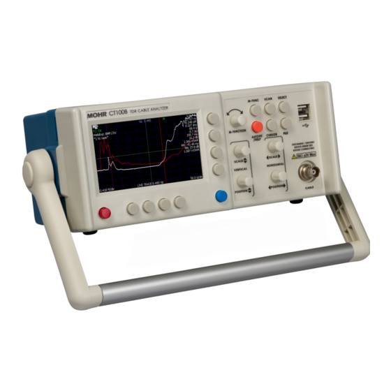
Page 1 Operator’s Manual: CT100B Series TDR Cable Analyzers For Software Version 2.24.5 Part No.: CT100B-M-OM-012 CAGE Code: 4JEE1 Revision Date: 2023.03.07...
Page 3: Copyright Notice
This manual may not be reproduced, distributed, transmitted, displayed, published, or broadcast in any form or medium by any other party without written permission from MOHR. MOHR products are covered by U.S. and foreign patents, issued and pending. Information in this publication supersedes all previously published material.
Page 5: Manual Updates
Manual Updates We at MOHR are always working to improve the written materials we offer to our valued customers. Since our last printing, there may have been minor updates to this manual. To view our most recent manual revision, open the accompanying CT Viewer 2 DVD, or visit us online at www.mohrtm.com.
Page 7: Warranty
MOHR. If any such product proves defective during this warranty period, MOHR, at its option, will either repair the defective product without charge for parts and labor, or will provide a replacement in exchange for the defective product. MOHR’s liability and Buyer’s remedies under this Warranty shall be limited solely to repair, replacement, or credit.
Page 9: Contacting Mohr
Contacting MOHR Phone +1-888-852-0408 Mail MOHR Test and Measurement LLC 2105 Henderson Loop Richland, WA 99354 Email Sales: sales@mohrtm.com Technical Support: techsupport@mohrtm.com www.mohrtm.com CT100B TDR Cable Analyzers Operator’s Manual...
Page 11: Table Of Contents
Storage ... 3.2.4. Low Battery ..Contacting MOHR 3.3. Labels ....
Page 12: Contents
Contents 4. Operating Instructions 5. Math Functions 4.1. Connecting Cable 5.1. Difference (Subtraction) Traces . . Device-Under-Test (DUT) ..5.2. First Derivative (Slope) Traces . . 4.2. Common Types of TDR Cable Faults 40 5.2.1. Second and Higher Order 4.3.
Page 13 Contents 7.8. VSWR ....102 C.2.2. Standard SMA Accessories 7.9. Rise Time and Spatial Resolution . 103 – CT100B (SMA), CT100HF122 7.10. Timebase/Cursor/Horizontal Res- C.2.3. Optional Accessories ..122 olution .
Page 15: List Of Figures
List of Figures 3.1. Example nameplate label found on back of a CT100B ....3.2. Diagram of the CT100B front panel ......3.3.
Page 16 List of Figures 4.29. The name of the currently selected annotation is displayed in the multifunction indicator 60 4.30. Using the on-screen keyboard ....... 4.31.
Page 17 List of Tables 3.1. SCAN Button and Menu ........3.2.
Page 19: General Information
1. General Information 1.1. Product Description The MOHR CT100B TDR Metallic Cable Analyzer uses a form of closed-circuit radar known as time-domain reflectometry (TDR) to test cables for defects or “faults”. The instrument applies a fast rise time broadband step signal to the cable under test and then measures the reflected voltage at very short time intervals.
Page 20: Unpacking And Initial Inspection
MOHR-authorized sales representative. 1.5. Repacking for Shipment In the event that the CT100B needs to be shipped to a MOHR-authorized service center for repair, calibration, or other service, contact MOHR for a Return Material Authorization (RMA) number. Affix a label to the outside of the shipping container indicating: •...
Page 21: Safety Summary
2. Safety Summary The safety information presented in this brief summary is only intended for operators of the CT100B. Safety information relating to specific circumstances is present throughout this manual and is not necessarily present in this summary. Please read this manual in its entirety before using the CT100B and take note of safety information not included in this summary.
Page 22: Symbols In The Manual
2. Safety Summary 2.3. Symbols in the Manual 2.4. Symbols on the CT100B 2.5. Static Charge Any cable or wire can carry a significant static electric charge that could damage the sensitive internal electronics of the CT100B. For this reason, it is essential to discharge the electrical conductors of any cable or device-under-test (DUT) by shorting them to each other or to earth ground before connection is made to the CT100B’s sampling circuitry.
Page 23: Fuses
CAUTION: Use of any power source other than the supplied external power adapter(s) could damage the instrument and may void the Warranty. Use only MOHR-approved accessories. WARNING: To reduce the risk of electric shock, disconnect all external cables before connecting the 24 VDC external power supply.
Page 24: Grounding The Ct100B
2. Safety Summary 2.8. Grounding the CT100B When the CT100B is connected to the external AC adapter, the CT100B chassis, front panel USB, screen, and controls are grounded through the grounding conductor of the power cord. To avoid electrical shock, it is essential that the protective ground connection is present when operating the unit under AC power.
Page 25: Do Not Remove Covers Or Panels
Contact your local authorities for safe disposal in your area, or you may return them to MOHR for recycling. WARNING: The battery pack must be replaced with MOHR pn: CT100- AC-B2700. Use of any other battery pack will damage the instrument and pose a danger of fire.
Page 26 2. Safety Summary CAUTION: User replacement of components is limited. Multiple Warranty seals are installed on components within the CT100B. Removal or damage of these seals voids Warranty. CT100B TDR Cable Analyzers Operator’s Manual...
Page 27: Getting Started
3. Getting Started If you would like a detailed explanation of TDR measurement theory and applications before using the CT100B, please read Section 7, TDR Measurement Theory. 3.1. Handling The CT100B is designed to meet the rigors associated with normal instrument use both in the field and on the benchtop.
Page 28: Caring For The Battery
3. Getting Started 3.2.1. Caring for the Battery The CT100B has an intelligent battery-charging circuit that dynamically determines the optimum charge rate and reverts to low-level trickle charge when the battery is fully charged. Charging is automatic and there are no charge-length restrictions. The battery should be charged between 0 C and +45 C.
Page 29: Labels
The correct code for a particular device can be requested from MOHR. Installation instructions will be included with the license code or can be found in Appendix E.5.
Page 30: Preparing To Use The Ct100B
3. Getting Started 3.5. Preparing to Use the CT100B Before using the CT100B, make sure you have read and understand the Safety Summary section and the power requirements described in Section 3.2. If you would like a detailed explanation of TDR measurement theory and applications before using the CT100B to test cables, please read Section 7, TDR Measurement Theory.
Page 31: Rear Panel Connectors And Switches
The following numbered items describe the connectors and switches identified in the rear panel diagram (Figure 3.3). 24. 24 VDC power adapter plug. The provided 24 VDC AC adapter plugs into this port. Only MOHR-approved positive center tip, 24 V adapters may be used. CT100B TDR Cable Analyzers Operator’s Manual...
Page 32: Keyboard Alternate Controls
3. Getting Started Figure 3.3. Diagram of the rear panel of the CT100B/CT100HF. 25. Client USB connection. Allows the CT100B to be connected to a host computer for data transfer and PC control. 26. RJ45 Ethernet port. This is a 10/100 Mb Ethernet port that can be used for data transfer and remote PC control.
Page 33: Menu Selections And Function Buttons
3. Getting Started Figure 3.4. Keyboard controls for front panel buttons and knobs. 3.9. Menu Selections and Function Buttons 3.9.1. M-FUNC Button The M-FUNC button is used to switch between functions Brightness, Shift, Smooth, and Vp (and Fine/Coarse Vp) shown in the Multifunction indicator at the top of the display screen. Brightness controls how bright the screen display is.
Page 34: Scan Button And Menu
3. Getting Started Table 3.1. SCAN Button and Menu Menu Selection Purpose/Action Saves selected trace to internal storage. Renames Save/Rename previously saved traces. Turns all traces invisible except the currently selected Showing Sel. Trace Only/Showing trace. Select again to set all traces visible. All Traces Hides all traces except the live trace.
Page 35: Math Menu
3. Getting Started 3.9.2.1. Math Menu The Math menu is a menu selection under both the SCAN button and the blue MENU button. Math menu selections are shown in Table 3.2. Table 3.2. Math Menu Menu Selection Purpose/Action FFT Tools ▷...
Page 36 3. Getting Started Table 3.2 (Continued) Math Menu Menu Selection Purpose/Action ▷ ▷ ▷ OSL Bases Visible When enabled, the Open, Short, and Load traces will appear on-screen. Disabling it removes them from the screen, eliminating excess on-screen clutter. ▷ ▷ ▷ Align Base Traces When enabled, the Open, Short, Load, and DUT traces may be aligned to each other based on the common part of the beginning of the trace.
Page 37: Select Button
3. Getting Started Table 3.2 (Continued) Math Menu Menu Selection Purpose/Action Creates subtraction trace from selected trace and base Difference trace (Difference = Selected – Base). Creates first derivative trace from selected trace. 1st Derivative Toggles first derivative trace smoothing. Der.
Page 38: Cursor Button
3. Getting Started Figure 3.5. The Reset Options menu. For more information on default and user configurations, see Section 4.10. The Reset Options menu can also be found by briefly pressing the red POWER button and choosing Reset Options when the shutdown dialog appears. It is also part of the CT100B’s startup screens.
Page 39: Blue" Menu Button And Top-Level Menu
3. Getting Started Table 3.3 (Continued) FILE Button and Menu Menu Selection Purpose/Action ▷ Select ......Select the highlighted custom cable type. Instrument settings change to reflect the cable Vp setting. Use to select a built-in cable type from the standard Reference Cable Types cable type library.
Page 40: The Two Versions Of The Main Menu
3. Getting Started Figure 3.6. The two versions of the Main menu. On the left is the Special menu and on the right is the Standard menu. Note that the menu selections across the bottom are exactly the same for both menus. Top-level menu selections are listed below in Table 3.4.
Page 41 3. Getting Started Table 3.4 (Continued) MENU Button and Menus Menu Selection Purpose/Action Adjusts the pulse timing for different length cables: Cable Len (part of Standard Main menu) ▷ Short ......For cables of up to approximately* 300 ft. (90 m) long. ▷...
Page 42 3. Getting Started Table 3.4 (Continued) MENU Button and Menus Menu Selection Purpose/Action ▷ Find CT Viewer Searches the local area network for running CT Viewer 2 programs. If successful, it establishes a connection. ▷ Manual Connect A dialog with a list of PCs that have previously been added is displayed.
Page 43 3. Getting Started Table 3.4 (Continued) MENU Button and Menus Menu Selection Purpose/Action ▷ ▷ Next Segment Selects the segment to the right of the currently selected segment. ▷ ▷ Reset All Vp Resets the Vp of all segments to 1.000. ▷...
Page 44 3. Getting Started Table 3.4 (Continued) MENU Button and Menus Menu Selection Purpose/Action ▷ Meas. Settings ▷ ▷ Autoset Vp ▷ ▷ ▷ Autoset Vp with Autofit Set Vp from a cable of known length using Autofit. ▷ ▷ ▷ Autoset Vp from Current Set Vp from a cable of known length using manual cursor positioning.
Page 45 3. Getting Started Table 3.4 (Continued) MENU Button and Menus Menu Selection Purpose/Action ▷ ▷ Clear Resets all Ω/(unit) settings. See Table 3.2: Math Menu. Math Settings ▷ Meas. Settings See Meas. Settings under Measurement menu above. ▷ Save Trace Default Name Allows creation of default name for saved traces.
Page 46 3. Getting Started Table 3.4 (Continued) MENU Button and Menus Menu Selection Purpose/Action ▷ ▷ DC Shutdown Sets the inactivity timeout for shutdown while the device is running on external DC supply. ▷ ▷ Battery Power Save Sets the inactivity timeout for power save mode while the device is running on battery.
Page 47 Normally this setting should not be changed. ▷ ▷ Processor Displays CPU information. ▷ ▷ Contact Displays contact information for MOHR. ▷ ▷ Auto Update On/Off Toggles Auto Update on/off. With Auto Update on, the CT100B will automatically check to see if it is running the current software version and notify the user if a new version exists.
Page 48 3. Getting Started Table 3.4 (Continued) MENU Button and Menus Menu Selection Purpose/Action ▷ ▷ Temp Comp Toggles display of Temp Comp autocalibration status. ▷ ▷ Min/Max Display Toggles display of min/max values for high-resolution sampling. ▷ ▷ Horiz. Vert. Ruler Toggles display of horizontal and vertical rulers.
Page 49: Setting Up The Ct100B
3. Getting Started Table 3.4 (Continued) MENU Button and Menus Menu Selection Purpose/Action ▷ AutoSmooth On/Off When on, the CT100B will automatically pick a smoothing value based on the observed noise. When off, the CT100B will use the user-entered smoothed value. 3.10.
Page 50: Display Features
3. Getting Started With the keyboard off the screen, select the OK menu option to accept all changes to the current dialog box and close the dialog box. Select the Cancel menu option to close the dialog box while canceling all changes. With a USB keyboard attached, entries can be changed directly.
Page 51: Setting Date And Time
3. Getting Started Figure 3.9. Screenshot showing typical features of the CT100B. 3.10.3. Setting Date and Time The date, time, and time zone must be accurately set for saved data in the CT100B to be correctly time-stamped. 1. Change the date and time by pressing the MENU button. This calls up the Main menu. 2.
Page 52: Temperature Correction
3. Getting Started 3.10.4. Temperature Correction The CT100B automatically adjusts for changes in temperature. This eliminates the need for a warm-up period. However, a stable temperature is required for some functions, such as performance checks. To view the internal temperature, go to MENU Settings Display and toggle on Temperature.
Page 53: A Small Fault In A Long Cable
3. Getting Started thousand foot cable is displayed on the screen, there is only one measurement about every two feet. 2. Normal: Sample resolution setting is chosen to match the cable length setting for good compromise of detail and speed. For SHORT length cable settings, the resolution is 5.34 ps (less than a millimeter) or better.
Page 54: Measurement Settings
3. Getting Started 3.13. Measurement Settings 3.13.1. Horizontal Units Horizontal distance measurements can be displayed in meters, inches, feet, yards, or centimeters. 1. Select MENU Measurement menu. 2. Select the Horiz. Units menu item to switch between the different unit options. All measurements and all traces are immediately updated to reflect the unit change.
Page 55: Relative Reflection Coefficient (Rrc) Method
3. Getting Started 3.13.3. Relative Reflection Coefficient (RRC) Method The CT100B measures the relative reflection coefficient between cursors. When the two cursors of the CT100B are positioned on either side of a change in impedance, this measurement is the reflection coefficient for that change. The relative reflection coefficient is displayed on-screen with a prefix of ∆mρ.
Page 57: Operating Instructions
Figure 4.1 shows a comparison test of a coaxial cable using clip lead adapters (red, top) and a controlled-impedance adapter (black, bottom). The clip lead adapter TDR trace is severely degraded. MOHR is able to supply controlled-impedance adapters for almost every type of cable and connector. CT100B TDR Cable Analyzers Operator’s Manual...
Page 58: Common Types Of Tdr Cable Faults
4. Operating Instructions Figure 4.1. Clip lead adapter (red, top) and controlled-impedance adapter (black, bottom) testing of 3 ft. coaxial cable with short termination. Active cursor is at the test port. Clip lead adapters introduce severe TDR trace distortion. 4.2. Common Types of TDR Cable Faults TDR cable faults include opens, shorts, and soft (or partial) faults.
Page 59: A Scan Of An Sma Connector
4. Operating Instructions Figure 4.3. Short faults appear as a pulse downward in the TDR trace. Short or open faults measured through long lengths of cable (hundreds of feet) will show long, shallow reflections on the TDR trace. Figure 4.4 shows a scan of an SMA interconnect. The trace has a spike at the connection.
Page 60: Change Velocity Of Propagation (Vp)
4. Operating Instructions 4.3. Change Velocity of Propagation (Vp) Vp is expressed as a fraction of the speed of light. See Section 7.4 Velocity of Propagation (VoP, Vp) for a detailed description of Vp. The current setting for Vp appears on the lower center of the screen. Press the M-FUNC button until the top-center information indicator reads Vp.
Page 61: Screenshot Showing Autofit Result
4. Operating Instructions 3. If using the Special Main menu, press the MENU button then Distance to Fault. If using the Standard Main menu, press the AUTOFIT/HELP button, then select the AUTOFIT menu item. The CT100B will display a trace that includes the beginning and the end of the test cable.
Page 62: Final Vp Of The Cable
4. Operating Instructions Figure 4.6. Use of the HORIZONTAL SCALE knob to improve Vp accuracy. 5. Press the M-FUNC button to set the M-FUNCTION to Vp, and adjust Vp using the M-FUNCTION knob until the CT100B distance measurement to the active cursor equals the physical measurement.
Page 63: Cable Type Library
4. Operating Instructions 4.5. Cable Type Library The CT100B has a library of common cable types and associated velocities of propagation. Vp for these cable types can be loaded from the library. The user can add custom cable types to the CT100B as well.
Page 64: Distance-To-Fault
4. Operating Instructions Figure 4.8. Smoothed vs. unsmoothed traces at very small vertical scales (0.7 mρ per vertical division). 4.7. Distance-to-Fault 4.7.1. Measure Distance-to-Fault (DTF) 1. Attach the cable to the test port. 2. Set Vp to match the Vp of the attached cable or select an appropriate cable from the cable type library.
Page 65: Autofit Cable. The Cable Termination Is A Short
4. Operating Instructions Figure 4.9. AUTOFIT cable. The cable termination is a short. 4. Note the “bump” in the middle of the cable in Figure 4.9. This is where two short test cables are connected with a BNC barrel connector. Position the active cursor on the reflection caused by this cable fault.
Page 66: Relative Distance And Dtf Measurements
4. Operating Instructions Figure 4.11. A horizontally zoomed-in view of the cable fault with active (solid) cursor at the start of the fault (“toe” region) and inactive (dashed) cursor at the peak of the fault. The DTF measurement is highlighted (red circle). 4.7.1.1.
Page 67 4. Operating Instructions Figure 4.12. Relative distance measurement between two small impedance “faults” caused by BNC connectors. In general, for the most accurate relative distance or time measurements between two faults, place the cursors on the “toe” region of the faults where the TDR trace is just beginning to rise above or fall below the cable characteristic impedance.
Page 68: The Set/Clear Zero Offset Button On The Display Menu
4. Operating Instructions Figure 4.13. The Set/Clear Zero Offset button on the Display menu. Figure 4.14. The Zero Offset menu. Note that the cursor position is currently at 0.537 m in this example. CT100B TDR Cable Analyzers Operator’s Manual...
Page 69: Multi-Segment Cable Dtf Measurements
4. Operating Instructions Figure 4.15. After choosing Set New Position, the cursor position is now at 0.000 m. This setting only affects the on-screen display and measurements of the trace. This will not change a saved trace, and the zero offset cannot be saved. To clear the zero offset, go to MENU Settings Display...
Page 70: Multi-Segment Cable Segment With Vp Of 0.400
4. Operating Instructions 7. The Distance-to-Fault measured by the cursor reflects multi-segment Vp as shown in Figure 4.16 and Figure 4.17. Figure 4.16. Multi-segment cable segment with Vp of 0.400 (red circle). Figure 4.17. Multi-segment cable segment with Vp of 0.850 (red circle). Multi-segment cable measurements can be saved like other traces to the CT100B’s internal storage to be retrieved at a later time.
Page 71: Scan A Cable
4. Operating Instructions 4.8. Scan a Cable The CT100B can scan a cable with user-defined resolutions. The user can optionally save these records into internal storage. CT100B scans differ from traditional TDR traces because they can be used to save detail at a much higher resolution than displayed on the screen. Cable scans can subsequently be reviewed at different levels of detail and compared to prior scans to identify subtle changes in cable or connector performance.
Page 72: Working With Traces
4. Operating Instructions A scanned trace is created using the smoothing factor that is set at the time of the scan. Because of this, high-resolution or highly smoothed scans may take a long time. During a lengthy scan, a menu will appear with a Cancel option. See Figure 4.19. Select Cancel to abort the scan. Figure 4.19.
Page 73: Selecting The Live Trace
4. Operating Instructions Figure 4.20. Selecting the live trace. Figure 4.21 shows the same three traces with a saved scan selected. The saved trace has been moved vertically using the VERTICAL POSITION knob so that it is easier to see. Figure 4.21.
Page 74: Annotate A Trace
4. Operating Instructions Figure 4.22. Selecting a difference trace. 4.9.2. Annotate a Trace Entire traces, individual points on a trace, or a range of points on a trace can be annotated. If an individual point on a trace needs to be annotated, move the active cursor to that point. If a range of points on a trace needs to be annotated, move the active and inactive cursors to the starting and ending points of the range.
Page 75: The Annotations Selection In The Scan Menu
4. Operating Instructions Figure 4.23. The Annotations selection in the Scan menu. Figure 4.24. The Annotations menu. CT100B TDR Cable Analyzers Operator’s Manual...
Page 76: Use Set Start Point To Annotate A Specific Point On A Trace
4. Operating Instructions Figure 4.25. Use Set Start Point to annotate a specific point on a trace. Figure 4.26. Use Set Start Point and Set End Point to annotate a range of points on a trace. To view a list of all annotations attached to a trace, go to SCAN Annotations List Annotations.
Page 77 4. Operating Instructions Figure 4.27. The List Annotations selection brings up a list of annotations associated with a trace. From this box, the annotation text can be viewed or modified or an annotation can be deleted. An annotation for a specific point will show up as an arrow on the trace at that point. Annotations for a range of points show up as arrows at the starting and ending points of the range, connected by a line.
Page 78: Store A Trace
4. Operating Instructions Figure 4.29. After an annotation is created, the multifunction indicator at the top of the screen displays the name of the currently selected annotation. To save annotations, go to SCAN Annotations Save Changes. If annotations were made to an unsaved trace, a prompt for a name to save the trace with will appear and the trace will be saved with the annotations.
Page 79: Using The On-Screen Keyboard
4. Operating Instructions Figure 4.30. Using the on-screen keyboard. Choose Hide Keyboard when finished. Then choose OK to save the trace with the name you entered. 7. Select the Hide Keyboard option on the menu when finished. Then choose OK to save the trace with the name you entered.
Page 80: Load A Trace (Cable Records)
4. Operating Instructions 1. Press the blue MENU button. The Main menu appears. 2. Choose Settings Save Trace Default Name. 3. A dialog box appears. See Figure 4.31. Press the Show Keyboard menu option to display the on-screen keyboard, or use a USB keyboard. 4.
Page 81: Transfer And Delete Traces
4. Operating Instructions Figure 4.32. Loading a trace. Some stored traces, such as FFT traces, require some re-calculation to fully load. This calculation is done automatically, but it may take several seconds. 4.9.5. Transfer and Delete Traces The CT100B has a large storage space, capable of holding thousands of scans. However, with continued use, CT100B storage will eventually fill up.
Page 82: User Configurations
4. Operating Instructions CT Viewer 2. These scans are then stored in the Windows computer for later retrieval, review, email, and analysis. See Section 6: CT Viewer™ and/or the CT Viewer™ 2 Quick User Guide for details on transferring traces to a computer using CT Viewer 2. 4.9.5.1.1.
Page 83: Save Configurations
4. Operating Instructions User Configurations can reduce operator error when configuring the TDR to make important measurements. For this reason it is recommended that User Configurations be used when setting up the CT100B for important measurements, such as quality-control checks on a cable manufacturing line.
Page 84: A Trace That Passes The Mask Test
4. Operating Instructions Figure 4.33. A trace that passes the mask test. Figure 4.34. A trace that fails the mask test. To create a mask, use the following procedure: 1. Create a cable scan or load a scan from internal storage that will be used to generate a mask. 2.
Page 85: Storing A Mask
4. Operating Instructions 4.11.1. Storing a Mask The CT100B is capable of storing thousands of masks. To do this: 1. With a mask already displayed select FILE Masks menu. 2. Select Load/Save Mask. This will open a dialog for saving, exporting, loading, and deleting masks.
Page 86: Deleting A Mask
4. Operating Instructions 2. Press the FILE button. The File menu appears. 3. Press the Masks option to enter into the Masks menu. 4. Select the Load/Save Mask option. A scroll dialog appears, showing all saved masks. 5. Use the M-FUNCTION knob to highlight the mask you wish to export. 6.
Page 87: Envelope Plot With Fill Mode
4. Operating Instructions 2. Select MENU Measurement menu. 3. Select Envelope Plot submenu. 4. Toggle Envelope Plot to On. 5. Use the Fill Mode On/Off option to toggle between Fill Mode and Frequency Density display mode. The CT100B can monitor a trace for extended periods of time with appropriate power management settings.
Page 88: Envelope Plot With Frequency Density Display
4. Operating Instructions Figure 4.36. Envelope Plot with Frequency Density display. Figure 4.37. Envelope Plot with Fill Mode, showing the range of impedance values at the cursor position (51.5–172.3 ohms, red circle). Envelope Plots can be saved as screenshots: 1. With an Envelope Plot on-screen, select Save Picture. 2.
Page 89: Improving Measurements
4. Operating Instructions 4. Press the Select button to load the screenshot. 5. After the screenshot has loaded, pressing the OK or Cancel button will remove the screenshot from the screen. Screenshots can also be exported to a USB drive for storage or to transfer to CT Viewer 2 or another CT100B.
Page 90: Cable Resistive Loss Correction
4. Operating Instructions instance, if you are using a 100 ohm differential pulse splitter balun to measure differential impedance of twisted-pair cable, then the center impedance should be changed to 100 Ω. The CT100B is now configured for enhanced accuracy impedance measurements across a wide range of impedances.
Page 91: Take A Screenshot
4. Operating Instructions Figure 4.38. Resistive cable loss correction, before. Note that the trace slowly rises. Figure 4.39. Resistive cable loss correction, after. Note that the trace is nearly horizontal. 4.14. Take a Screenshot To save a screenshot, first insert a USB drive into the CT100B. Then hold down the SELECT button and press the M-FUNC button to trigger the screenshot.
Page 92: Web Server
4. Operating Instructions 4.15. Web Server The CT100B is able to export raw data and images in real time over Ethernet. To enable this feature, follow this procedure: 1. Select MENU Settings Network Settings. 2. Toggle Web Server to On. 3.
Page 93: Remote Control
4. Operating Instructions multifunction indicator at the top of the screen. There are two extra buttons, an up arrow and a down arrow, that can make scrolling through lists easier on the live control. Figure 4.41. The live control display on the CT100B web page. Each button and knob on the front panel of the CT100B maps to buttons on this page, which can be used to control the CT100B remotely.
Page 95: Math Functions
5. Math Functions The CT100B includes various math functions that can help highlight cable issues, measure impedance change, or otherwise help with cable analysis. The following sections explain how to perform those functions. 5.1. Difference (Subtraction) Traces Difference traces are traces calculated from the subtraction of one trace from another trace. A difference trace can allow the operator to identify subtle changes in cable or connector performance.
Page 96: First Derivative (Slope) Traces
5. Math Functions Figure 5.1. Difference trace. Live (base trace, purple, top), comparison scan (red, middle), difference (blue, bottom) traces show 3.43 ohm excess impedance (red circle) on the live trace due to a loosened BNC connector. 5.2. First Derivative (Slope) Traces The first derivative trace can be used for two main purposes.
Page 97: Second And Higher Order Derivative Traces
5. Math Functions Figure 5.2. First derivative trace (yellow, bottom). 5.2.1. Second and Higher Order Derivative Traces The 1st Derivative function can be applied to First Derivative traces to create second (and higher) order derivatives. 5.3. Fast Fourier Transform (FFT) Traces The CT100B can calculate FFT frequency-domain information from live and scanned TDR traces.
Page 98: Return Loss (S ) Traces
5. Math Functions Figure 5.3. FFT trace (blue). The FFT plot was created from the section of the black live trace that is currently red. FFT traces can be stored, reloaded, and transferred to CT Viewer 2 just like normal scanned traces.
Page 99: Return Loss (S ) Options
5. Math Functions 7. Select S Calibration. After going through an informational message box, the S Calibration menu will appear and the CT100B will ask for the open terminator. Attach the open terminator and press Scan Open, or alternatively press Use Selected to use the currently selected trace as the open calibration standard.
Page 100: Return Loss
5. Math Functions 5.5.1. Return Loss (S ) Pre-Filter The Pre-Filter can reduce aberrations in the S trace. This can be combined with a Common Mode Subtraction (CMS) transform on the input traces. To enable or disable these settings, do the following: 1.
Page 101: Cursors
5. Math Functions 5.5.4. Time-Domain Gating, or Return Loss (S ) Between Cursors The CT100B is able to use time-domain gating (also called time windowing) to isolate features in the time-domain trace for analysis in the frequency domain using the S Between Cursors feature.
Page 102: Return Loss
5. Math Functions Figure 5.6. S between cursors with tightened connector showing average return loss of -34.3 dB from 756 MHz to 3 GHz. Figure 5.7. S between cursors with loosened connector showing average return loss of -26.7 dB from 756 MHz to 3 GHz (7.7 dB excess return loss compared with the tightened connector in Figure 5.6).
Page 103: Other Return Loss
5. Math Functions 3. Toggle Use Calibration Kit Standards to apply offsets and coefficients to the S trace. 4. Set the Characteristic Impedance in Ohms. This is defaulted to 50. 5. Enter the offsets and coefficient values provided with the Open-Short-Load Calibration Standards.
Page 104: Normalized Tdr Traces
5. Math Functions Figure 5.8. Using a phase stable cable to improve S-parameter measurements on short microwave cables. Use the phase stable cable (green arrow) and position the rightmost cursor to the left of the secondary reflections (red circle) occurring after the open or short at the end of cable under test (blue arrow) so that they are excluded.
Page 105: Layer-Peeling (Dynamic Deconvolution) Traces
5. Math Functions Figure 5.9 shows a normalized TDR trace (blue) with a short fault in a 50 ohm cable. The normalized trace shows reduced aberrations and more accurate relative reflection coefficient and impedance after the fault compared with the live TDR trace. Figure 5.9.
Page 106: Smith Charts
5. Math Functions Figure 5.10. Example layer-peeling trace (yellow, bottom) versus live TDR trace (white, top). The layer peeled trace reduces the impedance error in the final cable segment (green arrows) by ~80%. 5.9. Smith Charts The Smith chart is a useful graphical tool for plotting reflection coefficients and complex impedance values and can be used to simplify impedance matching.
Page 107: Smith Chart Representation Of Open Fault
5. Math Functions Figure 5.11. Smith chart representation of open fault (red arrow). Figure 5.12. Smith chart representation of short fault (red arrow). CT100B TDR Cable Analyzers Operator’s Manual...
Page 108: Smith Chart Representation Of A 50 Ohm Resistive Load
5. Math Functions Figure 5.13. Smith chart representation of a 50 ohm resistive load (red arrow). Figure 5.14. Smith chart of reactive 200 ohm load showing effect of reactive impedance at higher frequencies. Cursor (red arrow) shows impedance value calculated at DC (0 MHz). CT100B TDR Cable Analyzers Operator’s Manual...
Page 109: Ct Viewer
6. CT Viewer The CT Viewer™ 2 computer software for Windows desktop allows users of the MOHR CT100B TDR Cable Analyzer to transfer, view, and manipulate cable scans that have been saved on their instruments. This software package allows the user to select scans from a stored database that can contain thousands of scans and compare, subtract, or find the first derivative of any of the traces.
Page 110: Send Saved Traces Over Usb
6. CT Viewer 6.1.2. Send Saved Traces over USB 6.1.2.1. Set up USB Drivers on the Host Computer The USB drivers need to be set up only once for each computer. The USB drivers for the CT100B should have been installed with CT Viewer 2. It is possible to skip this step during the installation. If the drivers aren’t installed, Windows will inform the user when the CT100B is connected over USB.
Page 111: Options Under The Connect To Ct Viewer Menu
6. CT Viewer Figure 6.1. Options under the Connect to CT Viewer menu. Figure 6.2. Selecting Manual Connect in the Connect to CT Viewer menu will bring up a server menu. 6.1.3.3. Manual Connection the First Time 1. From the server menu, Select Add PC . A window with various server settings appears. 2.
Page 112: Using Remote Control
6. CT Viewer 6.1.3.4. Connecting After the First Time 1. Navigate to the MENU Connect to CT Viewer Manual Connect menu. A window showing all the stored server connections will appear. 2. Use the M-FUNCTION knob to highlight the connection for the computer. 3.
Page 113: Tdr Measurement Theory
7. TDR Measurement Theory The purpose of this section is to familiarize the operator with the basic premise of time-domain reflectometry measurement theory as part of using the CT100B instrument. 7.1. Time-Domain Reflectometry (TDR) TDR is a form of closed-circuit radar in which a transient test signal is injected into a device-under-test (DUT) such as a cable, and reflected voltages are measured at precise elapsed times to construct a TDR waveform or “trace”.
Page 114: Common Types Of Tdr Cable Faults
7. TDR Measurement Theory The reflection coefficient is the ratio of the amplitude of the reflected portion of the test signal to the amplitude of the incident test signal. The reflection coefficient (Gamma, ) is related to the impedance change (Z) at a given point in a cable according to: where Z is the impedance of the load (e.g., the device under test [DUT]) and Z is the source...
Page 115: A Short Cable Fault Shows A Downward Step Edge At The Location Of The Fault
7. TDR Measurement Theory Figure 7.2. A short cable fault shows a downward step edge at the location of the fault. Short or open faults measured through long lengths of cable (hundreds of feet) will show long, shallow reflections on the TDR trace because the cable preferentially attenuates higher frequencies in the test signal, degrading the rise or fall time of the reflected fault.
Page 116: Normal Sma Female Barrel Interconnect Measuring 52.1 Ohms
7. TDR Measurement Theory Figure 7.4 and Figure 7.5 for SMA and BNC type connections. Connector damage and corrosion can change the impedance profile of a connector over time, typically increasing the excess impedance of the connector. Periodic surveillance with TDR can be used to confirm connector performance.
Page 117: Velocity Of Propagation (Vop, Vp)
7. TDR Measurement Theory 7.4. Velocity of Propagation (VoP, Vp) As mentioned in previous sections, a transmission line, such as a coaxial cable, has uniform geometry with a characteristic signal propagation velocity. This velocity of propagation (Vp, VoP, or VP), sometimes also called the velocity factor (VF) or wave propagation speed, is the measure of the velocity of an electrical signal within a cable expressed as a fraction of the speed of light in a vacuum.
Page 118 7. TDR Measurement Theory where Z(t) is the impedance at time t, Z is the source impedance, and (t) is the reflection coefficient at t. This is the basis for the CT100B ohms-at-cursor measurements. It is important to note that impedance is nonlinear with respect to reflection coefficient, as shown in Figure 7.6. Figure 7.6.
Page 119: Return Loss
7. TDR Measurement Theory 7.7. Return Loss Return loss is another way of measuring impedance change in a cable. Return loss is given in decibels (dB) and is always calculated using the relative reflection coefficient. Return loss is related to the reflection coefficient by the formula: Return Loss = 20 log...
Page 120: Vswr
7. TDR Measurement Theory 7.8. VSWR Voltage standing wave ratio (VSWR) is a way of displaying reflection coefficient in a nonlinear way that emphasizes changes in cable impedance. VSWR is related to the reflection coefficient according to: VSWR = VSWR measures the ratio of the maximum-over-time amplitude of the nodes and anti-nodes of the standing wave off of a reflection.
Page 121: Rise Time And Spatial Resolution
7. TDR Measurement Theory VSWR can also be selected as the vertical scale for a trace. From the Main menu, go to the Measurement menu and select Vertical Units. 7.9. Rise Time and Spatial Resolution Spatial resolution is defined by the ability of the operator to distinguish the presence of two closely spaced faults on a TDR waveform.
Page 122: Timebase/Cursor/Horizontal Resolution
7. TDR Measurement Theory Figure 7.9. Simulated comparison of a 90 ps rise time TDR (green) and an 800 ps TDR (red) with respect to the ability to depict two 1 cm long, 75 ohm faults spaced 1 cm apart on a 50 ohm cable.
Page 123: Frequency-Domain Measurements
7. TDR Measurement Theory 7.11. Frequency-Domain Measurements 7.11.1. Scattering Parameters The scattering parameter or S-parameter approach to describing a device-under-test (DUT) assumes that a DUT is a black box network with N ports. The S-parameter matrix contains the complex reflection and transmission coefficients of the network, describing the amplitude and phase of reflected and transmitted values from each port in response to excitation of one or more of the ports.
Page 124: Return Loss (S )
7. TDR Measurement Theory Figure 7.10. Comparison of S return loss of a 2.4 GHz WiFi patch antenna measured using a handheld VNA (Agilent® FieldFox N9927A, green) and TDR (CT100HF, blue), showing good agreement from DC to ~8.3 GHz. Note bandpass in the 2.4 GHz region. 7.11.2.
Page 125: Normalized Tdr Traces
7. TDR Measurement Theory incident voltage trace is reflected back to the TDR instrument, insertion loss (S ) is half of the corresponding S return loss measurement in dB: Cable Loss CL = Again, this relationship is valid if the cable is terminated with a short or open. One drawback to this technique is that the round-trip insertion loss reduces the length of cable that can be tested over a given bandwidth relative to a 2-port measurement because the attenuation of the test signal is doubled.
Page 126: Smith Charts
7. TDR Measurement Theory for the presence of these multiple reflections and provides more accurate impedance values. This effect is most pronounced when there are multiple large impedance transitions in a cable assembly and at short and open faults. Figure 7.11. Layer-peeling scattering diagram relating measured TDR trace (V [t]) to actual impedance changes (Z[x]) and their associated actual reflection coefficients ( [x, t]).
Page 127 7. TDR Measurement Theory Figure 7.12. Impedance Smith chart relationships. CT100B TDR Cable Analyzers Operator’s Manual...
Page 129: Specifications
A. Specifications A.1. Electrical Specifications Characteristic Specifications Notes Reflected rise time, CT100B 150 ps typ, 200 ps max 10 to 90%, into 50 Ω 10-90% Reflected rise time, CT100B 100 ps typ, 150 ps max 20 to 80%, into 50 Ω 20-80% Reflected rise time, CT100HF 100 ps typ, 130 ps max...
Page 130 DC power supply 24 VDC, 2.5 A, positive 500 VDC isolation from tip. Use only the test port. MOHR-approved power supply. Battery pack 12 NiMH AA cells, fused Pack may wear out over at 2.5 A time.
Page 131: Environmental Specifications
A. Specifications Characteristic Specifications Notes Battery charge time Up to 4 hours (2.5 hours typ.) from fully discharged state Overcharge protection Charging discontinues once full charge is attained. Discharge protection Instrument turns off Software shutdown when prior to battery damage battery is low.
Page 132 A. Specifications A.4.2 FCC Compliance CT100B and CT100HF emissions comply with FCC Code of Federal Regulations 47, Part 15, Subpart B, Class A Limits. A.4.3 CT100B and CT100HF comply with MIL-PRF-28800F, MIL-STD-461F RE102, CE102, and IEC61000. A.4.4 Shock and Vibration CT100B and CT100HF comply with MIL-PRF-28800F (class 3).
Page 133: Operator Performance Checks
NOTE: If a CT100B fails any Operator Performance Check, it should be serviced by a qualified repair facility. B.2. Required Equipment Table B.1. Required Performance Check Equipment for CT100B Item MOHR part number Precision 50 Ω terminator CT100-AC-ER50-S Connector, SMA female to BNC male CT100-AC-ISFBM 50 Ω...
Page 134: Getting Ready
B. Operator Performance Checks Table B.2. Required Performance Check Equipment for CT100HF and CT100B with SMA Option Item MOHR part number Precision 50 Ω terminator CT100-AC-ER50-S Connector, SMA male to BNC female CT100-AC-ISMBF Shorting cap CT100-AC-ISS 50 Ω 36 in. reference cable...
Page 135 B. Operator Performance Checks B.4.3 Pulse Amplitude Check 1. Pulse amplitude measurement should be taken with a device that can accurately measure frequency, pulse width, period, and amplitude. 2. Set the device input impedance to 50 ohms. 3. Connect one end of the 36 in. reference cable to a capable pulse measurement device and the other end of the 36 in.
Page 136 B. Operator Performance Checks 3. Connect one end of the 36 in. reference cable to a capable pulse measurement device and the other end of the 36 in. reference cable to the CT100B front panel cable connector. A trace should appear on the device display. 4.
Page 137 B. Operator Performance Checks B.4.12 Cursor Readout Range Check 1. In the Measurement menu, toggle on Extra Long Mode. 2. Turn the HORIZONTAL SCALE knob counterclockwise until horizontal scale is maximized. 3. Using the M-FUNC button and M-FUNCTION knob, set Vp to 1.000. 4.
Page 138 B. Operator Performance Checks B.4.17 Vertical Accuracy Check (ohms) 1. Vertical accuracy is checked by comparing CT100B impedance measurements against a load of known impedance. The supplied 50 ohm terminator is required. 2. Within the Main Settings Display submenu, select the Ohms Rho button until Ohms is marked with asterisks.
Page 139: Options And Accessories
C. Options and Accessories C.1. Options Model CT100B (BNC) – self-grounding BNC test port Model CT100B (SMA) – stainless-steel SMA test port Model CT100HF – high-frequency sampler, stainless-steel SMA-type test port C.2. Accessories C.2.1. Standard BNC Accessories – CT100B (BNC) BNC 50 ohm 36 in.
Page 140: Standard Sma Accessories
C. Options and Accessories C.2.2. Standard SMA Accessories – CT100B (SMA), CT100HF SMA 50 ohm 36 in. Reference Cable CT100-AC-W536-S SMA 50 ohm Terminator CT100-AC-ER50-S SMA Male to Male Adapter CT100-AC-ISMM Connector, SMA Female to BNC Male CT100-AC-ISFBM Connector, SMA Male to BNC Female CT100-AC-ISMBF Connector, SMA Female Short CT100-AC-ISSF...
Page 141: P Of Common Cables
D. V of Common Cables D.1. Cable Types Commonly encountered cable designations, along with their associated characteristic impedances and typical Vp values, are listed below. A more complete listing is stored in the CT100B’s internal memory. Note that the actual Vp of a given cable can vary by manufacturer, manufactured lot, cable age and condition, whether it is flat or coiled on a roll, and other variables.
Page 142: Rg Standards
D. V of Common Cables D.3. RG Standards Table D.2. Vp of RG Standards Designation (ohms) RG-6/U 0.66 RG-6/UQ 0.66 RG-8/U 0.66 RG-9/U 0.66 RG-11/U 0.66 RG-58/U 0.66 RG-59/U 0.66 RG-62/U 0.84 RG-62A 0.84 RG-174/U 0.84 RG-178/U 0.69 RG-179/U 0.67 RG-213/U 0.66 RG-214...
Page 143: Commercial Designations
D. V of Common Cables D.5. Commercial Designations Table D.4. Vp of Commercial Designations Designation (ohms) H155 0.79 H500 0.82 LMR-200 0.83 HDF-200 0.83 CFD-200 0.83 LMR-400 0.85 HDF-400 0.85 CFD-400 0.85 LMR-600 0.87 LMR-900 0.87 LMR-1200 0.88 LMR-1700 0.89 D.6.
Page 145: Maintenance And Service Instructions
E. Maintenance and Service Instructions E.1. Cleaning and Lubrication Ensure that the CT100B power is off before cleaning. Clean the CT100B with a damp cloth. Clean the LCD screen with LCD screen cleaner or optical lens cleaner. Do not use any powerful solvents when cleaning the CT100B.
Page 146: Calibration And Calibration Interval
Note: If multiple license files are on a USB flash drive, the CT100B will reject the file. Make sure the intended license file is the only MOHR license file on the drive. 1. Copy the file to an empty USB flash drive. (Do not change the file name.) 2.
Page 147: Operator Troubleshooting
F. Operator Troubleshooting F.1. General Information Use this troubleshooting guide when there is a problem with a CT100B or to assist with problem identification. This will help you to determine if the instrument should be repaired or is acceptable to continue using. Any time one of the internal thermal fuses actuates with an audible click, indicating thermal overload, turn off the rear panel battery-disconnect switch immediately and have the instrument serviced as soon as possible.
Page 148 F. Operator Troubleshooting F.3.1 Functional Block Diagram 24 VDC charging Internal 12 Cell Client USB, from AC adapter NiMH Battery Pack Ethernet CT100-AC-PS CT100-AC-B2700 DC Power, Temperature Ethernet, Back Panel Assembly DC Power Client USB CT209B Analog Power W1W5C1 Ethernet W2W6C1, Client USB W2W6C3, Serial Port +5 V Digital...
Page 149 Time Clock FAIL Verification (F.3.9) PASS Perform File IO FAIL Verification (F.3.10) PASS Return to MOHR for Return to MOHR for factory diagnosis and factory diagnosis and Device is in working repair repair order CT100B TDR Cable Analyzers Operator’s Manual...
Page 150 F. Operator Troubleshooting F.3.3 External DC Diagnostics Start External DC Diagnostics Plug 24 volt DC Replace power supply power supply into a (CT100-AC-PS) wall socket Change to a working Does the AC AC wall outlet outlet work? Does the green Verify the power light on the supply is firmly...
Page 151 F. Operator Troubleshooting F.3.4 Startup Diagnostics Start Is the screen blank/white and unchanging for >1 minute? Did the MOHR splash screen appear? Did a progress bar appear? Is the progress bar frozen or reporting an error? Is the device locking up after...
Page 152 F. Operator Troubleshooting F.3.5 Front Control Verification Start Front Control Diagnostics Press the blue MENU button Choose Settings -> Does the Main Diagnostics menu menu appear? item. Choose Front Panel Check menu item Does the front panel diagnostics screen appear? Turn each knob left and right and press each button except...
Page 153 F. Operator Troubleshooting F.3.6 Analog Diagnostics Start Analog Diagnostics Install a valid license Did a message appear file by following the on the device stating instructions in that the license was out Appendix E of the of date or invalid? manual and restart the device.
Page 154 F. Operator Troubleshooting F.3.7 TDR Pulse Diagnostics Start TDR Pulse Diagnostics Return to Main Menu and navigate to SettingsàDiagnostics and select Analog. Attach a shorted terminator and press OK. Using an oscilloscope, verify the TDR pulse Did all tests characteristics as displayed pass? described in “Operator Performance Checks”.
Page 155 F. Operator Troubleshooting F.3.8 USB Client and Ethernet Verification Start Connect back USB to known working PC with CT Viewer 2 installed. Does the PC recognize the device? Connect known working Ethernet cable that is connected to a network to the device.
Page 156 F. Operator Troubleshooting F.3.9 Real Time Clock Verification Start Navigate to Main Menuà Settingsà Infoà Time. Change the date and time and select Turn power off, then restart the device. Does the device display the new time? Reset correct date and time.
Page 157 F. Operator Troubleshooting F.3.10 File IO Verification Start Verify that only the live TDR trace is on the display. Enclose the leading edge of the live trace with the two cursors and generate a cursor scan. See Section 4.8 for instructions on creating a scan. While in the Scan menu select Save.
Page 158: Parts List
F. Operator Troubleshooting F.4. Parts List Subassembly Item Part No. Qty. Description CT100B — CT100B — CT100B TDR Cable Tester CT291 Rear Housing CT292 Front Cover Front Panel Assembly — CT290B — LCD display, front control board, switches, cables, and knobs W2W7C1 Digicomp-video PCB FFC 40 pin flat- flex 0.5 mm space...
Page 159: Glossary
Glossary Aberrations Imperfections or undesired variations in a signal. For example, aberrations in a TDR’s excitation signal are the result of the finite switching speed of the instrument’s electronics and cause it to deviate from a perfect step signal. AC Alternating current, a method of delivering electrical energy by periodically changing the direction of the electric field in a conductor.
Page 160 Glossary dB dB is the abbreviation for decibel. Decibels are a method of expressing power or voltage ratios as logarithms. When used for voltage ratios, as in TDR, the formula for decibels is dB = 20 log ) where V is the voltage of the incident pulse and V is the voltage reflected back by the load.
Page 161 Glossary IP Internet Protocol. The universal protocol used to send data through the internet. Also used in many other computer networks. Each computer on a network must have a unique IP address. Jitter The uncertainty in measurement of time in a TDR. The main effect of jitter is to cause apparent vertical noise in areas of changing impedance.
Page 162 Glossary Reflectometer An instrument that measures reflections to determine the state of a system. The CT100B measures the reflections of electrical energy. Resistance A conductor’s opposition to electrical current. The reciprocal of resistance is conductance. Electrical resistance can often be considered a constant that does not vary with respect to the voltage or current applied to an object.
Page 163 Glossary considered a complete characterization of a linear device for the frequency range of the scattering parameters. Short Circuit The condition in which the conductor in a cable or circuit comes into direct contact with the return path conductor or earth ground. The electrical length of the cable measured by TDR is shortened to the point of the short circuit.
Page 165: Index
Index .csv, 64 MENU, 12, 21 POWER, 12 AC power, 1, 5 SCAN, 13, 15, 60 adapter plugs SELECT, 13, 19 voltage, 9 V1, 13 add server, 93 V2, 13 annotations, 56 V3, 13 assistant mode, 94 V4, 13 auto-update, 29 cable fault balun common types, 40, 96...
Page 166 Index connecting over Ethernet, 92 impedance, 99 movie, 94 at cursor, 48 remote control, 75, 94 resistive loss correction, 72 working with USB drive, 91 toggle on/off, 29 impedance-matching adapters, see vertical damage reference calibration due to electrostatic discharge, 9 insertion loss due to static charge, 4 frequency domain (S...
Page 167 Index menu return loss (S ) options, 81 AUTOFIT/HELP, 19 aberration filter, 82 FILE, 20 align base traces, 85 Info, 11 between cursors, 83 Math, 17 calibration standards, 84 Power, 10 hide calibration traces, 85 SCAN, 15 noise filter, 82 Special, 21 phase correction, 82 Standard, 21...
Page 168 Index temperature velocity of propagation correction, 34 AUTOFIT/HELP button, 43 operating, 9 changing the value of, 42 storage, 9 finding an unknown, 42 temperature correction, 34 for common cable types, 123 thermal breakers, 5 load a cable type’s Vp, 45 time-domain gating, 83 load and save custom cable types, 45 time-domain reflectometry, 1, 95...

Mohr CT100B Series Operator's Manual

Quick Links

Need help?

Questions and answers

Subscribe to Our Youtube Channel

Related Manuals for Mohr CT100B Series

Summary of Contents for Mohr CT100B Series

Table of Contents