Page 1 MCA4A 4 Input Multichannel Analyzer 2 Input Multichannel Scaler User Manual © Copyright FAST ComTec GmbH Grünwalder Weg 28a, D-82041 Oberhaching Germany Version 2.09, October 25, 2018...
Page 2 ComTec GmbH...
Page 3 You have purchased the license to use this software, not the software itself. Since title to this software remains with FAST ComTec, you may not sell or transfer this software. This license allows you to use this software on only one compatible computer at a time. You must get FAST ComTec's written permission for any exception to this license.
Page 4: Table Of Contents
2.5.3 Simple Pulse Height Analysis...................... 19 2.5.4 Measuring a typical Pre-Amplifier Signal..................22 2.5.5 Multiscaling measurement......................26 2.5.6 Basic Usage of the RealTimeClock Option..................28 2.6 Installing more than one MCA4A Module.....................29 3 Hardware Description..........................31 3.1 Overview.............................. 31 3.2 Front Panel Connectors........................31 3.2.1 Analog ADC Inputs........................
Page 5 5.1 File Menu............................. 74 5.2 Window Menu............................77 5.3 Region Menu............................78 5.4 Options Menu............................84 5.5 Action Menus............................95 6 Programming and Software Options......................97 7 Appendix..............................98 7.1 Absolute Maximum Ratings......................... 98 7.2 Recommended Operating Conditions....................98 7.3 Specifications............................98 7.3.1 ADC inputs...........................
Page 6 Fig. 2.2: Driver Installation..........................11 Fig. 2.3: Choosing the right folder........................12 Fig. 2.4: Device Manager after successful driver installation................12 Fig. 2.5: MCA4A rear panel..........................13 Fig. 2.6: Software startup screen........................14 Fig. 2.7: MCA4A Settings window........................14 Fig. 2.8: ADC Settings dialog (2x)........................15 Fig.
Page 7 Fig. 4.12: Setting a ROI in the waveform for the pulse-height analysis of flattop pulses.........50 Fig. 4.13: How to switch off Auto Scaling ....................... 50 Fig. 4.14: Setting parameters for flattop PHA....................50 Fig. 4.15: Pulse Width Histogramming......................51 Fig. 4.16 Scaler Settings dialog box....................... 52 Fig.
Page 8 ComTec GmbH...
Page 9: Introduction
The 32 bit or 64 bit MPANT Windows Software is able to handle 6 MCA4A providing up to 24 MCA channels. In-field upgrade options enable upgrading of MCS mode, more MCA channels, 8 ns RTC time tagging, and multiparameter coincidences for 2 or 4 ADCs including Replay of list files.
Page 10: Installation Procedure
2.1 Hard- and Software Requirements For operating the MCA4A you need a standard PC with a high-speed USB 2.0 or USB 3.0 port and Microsoft Windows XP or higher. USB 1.0 ports do not work. The maximum throughput rate is approximately 32 Mbyte/sec on a USB 2.0 port and 120 Mbyte/sec on a USB 3.0 port.
Page 11: Driver Installation
Installation procedure 2.2 Driver Installation To install the driver, please start the device manager. You can do it by right-clicking the computer shortcut on the desktop and selecting ”Manage” from the drop-down-menu, then ”Device Manager”. Another way is to select in the Start Menu Settings..Control Panel, then System..Device Manager. Fig.
Page 12: Fig. 2.3: Choosing The Right Folder
If there is a exclamation mark at the driver and there is an error message that the device could not start, please remove the power from the MCA4A device and reconnect it. If you don't see the device at all, it is possible that the USB3 driver must be updated.
Page 13: Software Installation
USB cable into a high-speed capable USB port. Since USB is a hot-pluggable interface the sequence of applying power and connecting the USB port is not important. When the power is applied the “POWER ON” LED on the rear of the MCA4A should be lit and a second later “POWER GOOD” as well.
Page 14: Getting Started
First step is to start the MCA4A software by double clicking the corresponding icon. This will automatically start the MPANT program as well. On startup the MCA4A Server is iconized and one does not have to worry about it since all hardware settings are accessible from the MPANT program which actually is the graphical user interface and which will appear now on your screen.
Page 15: Fig. 2.8: Adc Settings Dialog (2X)
Fig. 2.8: ADC Settings dialog (2x) Make sure you have no signals connected to the MCA4A inputs! Click Get Zero and then Apply to perform a measurement of the input offsets. The zero value is expected to be somewhere around 3,200.
Page 16: Basic Scope Measurement
A calibration of the internal offsets (zero values) for all input ranges (pos. unipolar, bipolar and neg. unipolar Pulse polarity) should be performed at the first startup Please let the MCA4A warm up for some 30 minutes before calibration is performed 2.5.2 Basic Scope measurement This might be the best thing to start with.
Page 17: Fig. 2.10: Scale Parameters For The Scope Display
Installation procedure Before we will start the measurement we first set the display windows scalings. Click on the scope display window (A1 (3) in Fig. 2.12) to make it the active window in MPANT. Select Options – Scale parameters... or click and set the Counts Range to 0 …...
Page 18: Fig. 2.12: 1St Scope Measurement
Installation procedure Fig. 2.12: 1st scope measurement In the upper client window (A1) you see the scope picture of our square wave while in the lower (a_1) the spectrum of the analysed pulse height is displayed. Holding the left mouse button in a display window does set and move the cursor which values are shown just below the x-scale.
Page 19: Simple Pulse Height Analysis
Installation procedure Here select Custom Formula... to get the Custom-transformed spectra setup. Choose Formula #: 6 (ref. Fig. 2.14, left side) which is the FFT and click Create. Fig. 2.14: Setup a FFT analysis This creates a third display window containing the Fast Fourier Transformation data (ref. Fig. 2.15). Most probably you might want to switch the scaling from linear to logarithmic or vice versa (use the button).
Page 20: Fig. 2.16: Setup A Gaussian Fit Pha Measurement
Installation procedure Fig. 2.16: Setup a Gaussian Fit PHA measurement Select Action1 – Start or click and start the scope measurement - halts the measurement. The resulting picture is in Fig. 2.17. You clearly see the sine wave with 1MHz and 6V amplitude.
Page 21: Fig. 2.18: Switch To Firmware Based Pha
Installation procedure Again go to the ADC Settings and Presets dialog and deselect Scope-Mode (ref. Fig. 2.18). Fig. 2.18: Switch to firmware based PHA Now only one display (the PHA spectrum) remains in the MPANT window. After starting the measurement again a peak begins to rise approximately at channel 5559 and you can see a data rate of almost 1MHz.
Page 22: Measuring A Typical Pre-Amplifier Signal
Installation procedure 2.5.4 Measuring a typical Pre-Amplifier Signal We will now use the MCA4A's internal test pulser to produce pre-amplifier like input signals and setup the pole zero filter and the trapezoidal shaper. Since most pre-amplifier signals are typically negative we switch to the negative unipolar pulse polarity and use the scope mode to see how the input signals look like.
Page 23: Fig. 2.20: Setup The Internal Test Pulser
Installation procedure Fig. 2.20: Setup the internal Test Pulser Starting the measurement we see the negative going input pulses as in Fig. 2.21. Fig. 2.21: Scope Picture of the original Test Pulser Signals Now switch to Firmware based shaping (ref. Fig. 2.22). This inverts the input signals which is necessary since the firmware based shaping and pulse height analysis procedures are applicable for positive going pulses only.
Page 24: Fig. 2.22: Scope Picture Of The Internal Test Pulser
Installation procedure Fig. 2.22: Scope Picture of the internal Test Pulser Now we can see positive going, inverted signals that are applicable to the firmware shaping and analysis procedures. Fig. 2.23: Scope Picture of the inverted and positive going Test Pulser Signals ComTec GmbH...
Page 25: Fig. 2.24: Enable The Trapezoidal Filter
Installation procedure In the ADC Settings dialog enable the Trapezoidal Filter (ref. Fig. 2.24). Fig. 2.24: Enable the Trapezoidal Filter The resulting scope picture shows the trapezoidal shaped pre-amplifier pulses as in Fig. 2.26. With the now open Pole Zero Adjust window you may change the settings of the pole zero filter and optimize the resulting shaped pulse form.
Page 26: Multiscaling Measurement
Installation procedure Also try to optimize the Peaking and Gap samples. In Fig. 2.27 you see the resulting waveform with Peaking samples = 40 and Gap samples = 80. Fig. 2.27: Modified shaper parameters 2.5.5 Multiscaling measurement To setup a simple multiscaling measurement we need a square wave generator that provides 2 synchronous signals.
Page 27: Fig. 2.29: Mcs Settings For A Simple Measurement
Installation procedure Fig. 2.29: MCS Settings for a simple measurement Set Range = 1024, Dwelltime = 100ns, MCS Inputs Polarity to TTL, Impedance = 50 Ohm and click OK. After starting the measurement a garden fence like spectrum begins to grow (ref. Fig. 2.30). The distance of the peaks is 100 channels corresponding to 100 x 100ns = 10µs or 100kHz.
Page 28: Basic Usage Of The Realtimeclock Option
Installation procedure 2.5.6 Basic Usage of the RealTimeClock Option To familiarize with the usage of the RealTimeClock (RTC) option a simple experiment is setup. The intention is to measure the arrival time of single ADC events relatively to a start (trigger) signal like it might be done in Time-of-Flight or similar experiments.
Page 29: Installing More Than One Mca4A Module
2.6 Installing more than one MCA4A Module The software is able to operate up to 6 MCA4A modules with a single computer. Just connect them at an USB port, switch on the power, and install the driver when you are prompted. When starting the software, you will be asked to edit the MCA4.INI file as more than one MCA4A modules are found, and the notepad...
Page 30: Fig. 2.35: Editing Mca4.Ini
Installation procedure Fig. 2.35: Editing MCA4.INI That is all you have to do, next time when you start the software all modules will be found and can be operated. ComTec GmbH...
Page 31: Hardware Description
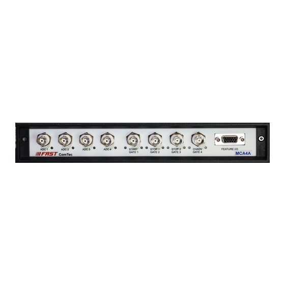
3.2.1 Analog ADC Inputs The analog ADC inputs are 4 BNC type connectors on the front panel of the MCA4A. Each is paired with a green LED that indicates that the input is active. They accept negativ or positiv uni-polar or bi-polar signals.
Page 32: Changing The Input Range
Hardware Description 3.2.2 Changing the Input range The full scale voltage range is jumper selectable between 2.0V, 2.5V, 8.0V and 10.0V (default). Fig. 3.2: Left: jumper setting for different input ranges, right: jumper positions The default setting is 10 V corresponding to a VPP value of 11019 (mV) for the full 16 bit range 0..65535. This value can be edited in the ADC settings, if the “advanced Settings”...
Page 33: Gate / Mcs Inputs
Hardware Description 3.2.3 GATE / MCS Inputs The GATE / MCS inputs provide a switchable 4.7kOhm pullup to +3.3V, 4.7kOhm pulldown to GND or 50Ohm to GND input impedance. Each input is equipped with a fast discriminator. The threshold level can be chosen from +1.3V for TTL signals or -300mV for fast NIM signals.
Page 34: Feature I/O Connector
Hardware Description 3.2.4 FEATURE I/O Connector Fig. 3.5: Circuit diagram of the FEATURE I/O port Single-channel-analyzer (SCA) Outputs When a maximum of the sampled analog ADC data is detected the corresponding maximum value is evaluated for lower- and upper-level thresholds (LLD and ULD). If the maximum falls in between LLD and ULD the pulse is accepted as valid and a SCA output pulse of 120 ns is initiated.
Page 35: Mca Section, Analog-To-Digital Converter
Hardware Description Fig. 3.6: Digital I/O port details GO-Line The system-wide open-drain wired-AND 'GO-Line' enables any connected device to start and stop all participating measurment equipment simultanously. The 'GO' line may be enabled, disabled, set and reset under software control. Fig.
Page 36: Pulse Height Analysis
Hardware Description The available trigger modes are SINGLE, NORMAL and AUTO. In SINGLE mode only the first trigger event is displayed. In NORMAL mode subsequent trigger events start a new display. In AUTO mode the measurement is triggered by real trigger events or - in absence of those - automatically.
Page 37: Fig. 3.9: Gaussian Shaped Pulse Fitting
Hardware Description Fig. 3.9: Gaussian shaped pulse fitting The conversion time (ref. chapter 7.4.2 ) depends on the number of samples used for the fit. NOTE: The optimum number of samples used for the fit depends on the shaping time of the input pulses. Flat top pulse fitting: For flattop pulses a chosen number of samples is averaged.
Page 38: Sampled Voltage Analysis
Hardware Description Fig. 3.11: Pile-up detection A second option to discard pile-up events is to use the GATE input as REJECT signal if the external electronics (e.g. pre-amplifier) provides such a signal. In this mode an active REJECT signal while the ADC input signal is above the threshold (i.e.
Page 39: Multichannel Scaler
Hardware Description 3.4 Multichannel scaler 3.4.1 Introduction In MCS mode of operation the MCA4 counts STOP events relative to the START (trigger) signal. The time resolution is equal to the selected dwell time. The total measurement time is the spectrum length in time bins multiplied by the dwell time.
Page 40: Octal 125 Mhz Counter / Timer
3.5 Octal 125 MHz Counter / Timer The MCA4A includes eight 48bit synchronous 125 MHz up-/down-counters. 2 counters are presettable. All inputs are TTL like and are terminated with 50Ω to ground. For each counter input the polarity is software selectable.
Page 41: Software Description
The window of the MCA4 server program is shown here. It enables the full control of the MCA4A to perform measurements and save data. This program has no own spectra display, but it provides - via a DLL (”dynamic link library”) - access to all functions, parameters and data.
Page 42: Action Menus
Software Description Fig. 4.2: MCA4.ini File 4.1.2 Action menus The server program normally is shown as an icon in the taskbar. After clicking the icon it is opened to show the status window. Using the “Start” menu item from the Action1 menu a measurement can be started. In the status window every second the acquired events, the counting rate and the time are shown.
Page 43: Fig. 4.3: Data Operations Dialog For Mpa Data (Left) And Selected Spectra (Right)
Software Description Fig. 4.3: Data Operations dialog for MPA data (left) and selected spectra (right) The menu item File – Replay... opens the Replay dialog. It enables evaluation of list data. The Replay software licence is usually programmed into the MCA4 module or by an optional USB dongle. Fig.
Page 44: Settings Overview
MCA4A.SET for the first MCA4 module.
Page 45: Mcs Settings
Software Description 4.1.5 MCS Settings Fig. 4.7: MCS Settings for one (left) or two stop inputs (right) Clicking the MCS Settings button opens the MCS Settings or MCS2 Settings dialog as shown in Fig. 4.7. The Range defines the number of time bins, the Dwelltime can be set in units of 10 ns from 30 ns (MCS) or 50 ns (MCS2).
Page 46: Presets
Software Description For the MCS Inputs the Polarity can be selected between TTL and ECL (NIM) signals. For each of the MCS inputs you can select between the rising and the falling edge. Usually for TTL signals, rising edge should be active and for (negative) fast NIM signals “rising edge”...
Page 47: Adc Settings
The offsets will be saved into the default settings file MCA4A.SET by clicking “Save” in the hardware settings dialog, and automatically reloaded when the software is started next time. See chapter 2.5.1. As the offset calibration can cause a shift in the spectrum, be careful not to do a new “Get Zero”...
Page 48 The MCA4A is able either to record the waveform and send the complete waveform data (Scope Mode) or to do a pulse height analysis and just send the result. The maximum count rate is of course much lower in Scope mode, therefore this mode is used for optimizing the electronics like adjusting a pole zero in the amplifier and also selecting the parameters for the PHA (pulse-height analysis).
Page 49: Fig. 4.11: Left: Setting Tag Bits, Right: Advanced Settings
Software Description Fig. 4.11: Left: Setting Tag bits, right: advanced Settings If you check advanced Settings more options will appear for the PHA parameters. VPP (mV) is the voltage corresponding to the full range of the ADC from 0 to 65535 LSB's. You can change it if you have a calibrated value for example by connecting a DC voltage to the ADC input that is known very well for example by using a good digital volt meter.
Page 50: Fig. 4.12: Setting A Roi In The Waveform For The Pulse-Height Analysis Of Flattop Pulses
Software Description on the electronics creating the flattop pulses, which method of anchoring the ROI gives the best result for a varying pulse height. Fig. 4.12: Setting a ROI in the waveform for the pulse-height analysis of flattop pulses Fig. 4.13: How to switch off Auto Scaling Fig.
Page 51: Pulse-Width Histogramming
Software Description 4.1.8 Pulse-width histogramming The pulse width of the analog input pulse at the threshold level can be measured in units of 64 ns, the pulse width data is inserted into the highest 12 bits of the RTC data, the length of the timestamp data is then only 32 bits instead of 44 bits.
Page 52: Scaler Setting
Software Description 4.1.9 Scaler Setting The “Scaler Settings...” button in the settings overview opens the respective dialog box to define the use of the 8 125 MHz Scaler/Counters. This is an option, see chapter 3.5 . A utility program mca4scal.exe is started automatically and shows the scaler values, optionally as a ratemeter.
Page 53: System Definition
Software Description 4.1.10 System Definition The “System...” item in the settings menu opens the System Definition dialog box. S everal MCA's can be combined to form up to 4 separate systems that can be started, stopped and erased together. The use of the Digital Input / Output and the GO-Line can be defined: It can be used either to show the ON or OFF status of the systems if the checkbox Status Dig 0..3 is marked.
Page 54: Calculated Spectra Dialog
Software Description 4.1.11 Calculated Spectra dialog Dependent on installed options like RTC and Coincidence Mode the MCA4 software allows to create several calculated spectra from different channels. By clicking "Spectra..." in the Settings menu or the corresponding MPANT toolbar icon the Dualparameter and Calculated Spectra dialog box of the MCA4 server is called.
Page 55: Fig. 4.21: Multi Time Display Setting, Left With Installed Rtc Option And Right Without Rtc Option
Software Description point marks the lower left corner of the zoomed map, and the Compr. by 2^n means the power of two by which the spectra are compressed. A value of zero means full resolution. Fig. 4.21: Multi Time Display Setting, left with installed RTC option and right without RTC option. Press Add Time to define a new Time spectrum in the Multi Time Display Settings dialog.
Page 56: Fig. 4.22: Calculated Spectrum Setting, With (Left) And Without (Right) Rtc And Coincidence Options
Software Description Fig. 4.22: Calculated Spectrum Setting, with (left) and without (right) RTC and Coincidence options You have a choice between several formulas to combine two parameters: Sum = left + right makes a sum spectrum, and Diff = Range + left - right can be used to subtract two spectra. The Range and Name can be defined in the edit fields or default values will be taken.
Page 57: Fig. 4.24: Sum Of Counts Spectrum Before And After Calibration
Software Description In the "Sum of counts" dialog you can select which ADCs will contribute to the superdetector. It is recommended to enable "Use Calibration" and to perform a careful calibration of all selected ADC's: Make a short acquisition using a pulser or a calibration source so you get a peak in each used ADC. In each ADC zoom into the spectrum, then by keeping the right mouse button pressed drag from left to right over the peak to mark a fit region and click on the "Fit"...
Page 58: Conditions
Software Description 4.1.12 Conditions If the RTC and Coincidence options are enabled, press Conditions... from the "Dualparameter and Calculated Spectra" dialog to define or edit ROI Conditions in the Conditions dialog. Fig. 4.25: Conditions To define a new condition, press Add Roi... to open the ROI Condition dialog. Fig.
Page 59: Fig. 4.28: Conditions Dialog With Tag Bits Enabled
Software Description Here a Condition can be defined as a combination using the Boolean operators NOT, OR or AND of already defined conditions. The OR will be symbolized in the automatically generated name by a plus sign "+", the AND by an asterisk "*". If tag bits are enabled in the user licence, it is also possible to define tag bit conditions.
Page 60: File Formats
Software Description 4.2 File formats The .mpa format is used to save all spectra in a single file. It starts with an ASCII header containing the settings and then the spectra follow one after the other, each proceeded with a header line like [DATA0,16384 ] (This means the first single spectrum with a length of 16384 channels.) [DATA1,16384 ]...
Page 61 Software Description The software adds at the end of a list file a small data block containing the counter values. The format follow the scheme of scope mode data, it can be distinguished by the waveform length that is only 12 16-bit words. The lowest two bits 0 and 1 are the channel number 0..3 for ADC1..ADC4.
Page 62: Control Language
A sequence of commands that are stored in a file with extension .CTL can be executed by the MCA4 server program or MPANT with the “Load ” or “Run” command. Also the configuration files MCA4A.SET or the header files with extension .MP contain such commands to set the parameters. Each command starts at the beginning of a new line with a typical keyword, the case is ignored.
Page 63 Software Description ; bit 10: GO Low at Stop ; bit 11: Clear before triggered start digval=0 ; 0..255 DIG I/O Output value trigger=6 ; bit 1..4 control_trigger for scope mode. ; bit 0: TRG_EDGE_DOWN ; bit 1: TRG_EDGE_UP ; bit 2..4: TRG_SRC,0=none (softw.), 1..4=CH1..4, 5=extern ;...
Page 64 ; calibration unit caluse=0 ; bit 0=1: use calibration, higher bits: calibration formula [ADC2] ; the following section concerns parameters of ADC2 The following commands perform actions and therefore usually are not included in the MCA4A.SET file: ComTec GmbH...
Page 65 Software Description start ; Clears the data and starts a new acquisition of system 1. ; Further execution of the .CTL file is suspended until any ; acquisition stops due to a preset. halt ; Stops acquisition of system 1 if one is running. cont ;...
Page 66 Software Description loadcnf configfile ; Loads a configuration stored in a config file like mca4a.set. run controlfile ; Runs a sequence of commands stored in controlfile. This ; command cannot be nested, i.e. it is not possible to execute ; a run command from the controlfile called with a run command, ;...
Page 67 Software Description deleteallrois MC_# ; allows to delete all ROIs of a specified spectra (1 for # means ; A1..). The following commands make sense only when using the serial line or TCP/IP control or DLL control interface: MC_A? ; Sends the status of MC_A via the serial port and make it actual. MC_H? ;...
Page 68: Controlling The Mca4 Windows Server Via Dde
Software Description 4.4 Controlling the MCA4 Windows Server via DDE The MCA4 program can be a server for DDE (Dynamic Data Exchange). Many Windows software packages can use the DDE standard protocols to communicate with other Windows programs, for example GRAMS, FAMOS or LabVIEW.
Page 69: Fig. 4.31: Executing A Mca4 Command From A Labview Application
Software Description Fig. 4.31: Executing a MCA4 command from a LabVIEW application The MCA4 program then executes the command and, after finishing, it sends an Acknowledge message to the DDE client. This can be used to synchronize the actions in both applications. DDE Request The DDE Request is a message exchange to obtain the value of a specified item.
Page 70: Close Conversation
Software Description Fig. 4.33: Getting the data with LabVIEW 4.4.3 Close Conversation After finishing the DDE communication with the server program, it must be closed. Fig. 4.34: Closing the DDE communication in LabVIEW The following figure shows the “Panel” of the described VI for LabVIEW. ComTec GmbH...
Page 71: Fig. 4.35: Control Panel Of The Demo Vi For Labview
Software Description Fig. 4.35: Control Panel of the demo VI for LabVIEW ComTec GmbH...
Page 72: Controlling The Mca4 Windows Server Via Dll
Software Description 4.5 Controlling the MCA4 Windows Server via DLL The MCA4 server program provides access to all functions, parameters and data via a DLL (“dynamic link library”). So the server can be completely controlled by the MPANT software that provides all necessary graphic displays.
Page 73: Mpant Software
MPANT Software 5 MPANT Software The window of the MPANT program is shown here. It enables the full control of the MCA4 via the server program to perform measurements and save data, and shows the data on-line in several windows. Fig.
Page 74: File Menu
MPANT Software Fig. 5.2: MPANT Map and Isometric display A toolbar provides fast access to many used functions in the menu. A status bar at the bottom gives help about the meaning of the toolbar icons. A cursor appears when clicking the left mouse button inside the graphics area.
Page 75: Fig. 5.3: File New Display Dialog
MPANT Software The data read from a file is shifted according to the calibration, if it is available and 'Use Calib' is checked in the MCA4 Data Operations dialog, see Fig. 4.3. This dialog can also be used to load spectrum data from a file into an existing display window.
Page 76: Fig. 5.4: Compare Dialog
MPANT Software Compare... The Compare... menu item opens a dialog that enables to show two spectra with different colors in the same window. The active display window can be checked as a primary window and there is a list of other spectrum windows that can be inserted as secondary windows.
Page 77: Window Menu
MPANT Software Print... The Print menu item opens the print dialog. It allows to arrange several pictures on a page into zones. The number of zones in vertical and horizontal direction can be specified. The Color can be black/white, RGB (colored) or Gray scale.
Page 78: Region Menu
MPANT Software Open All By selecting the Open All menu item, all Display windows are opened. Window list At the end of the Window menu, all created Display windows are listed with their names, the current active window is checked. By selecting any of the names, this window becomes the active window and is displayed in front of all the others.
Page 79 MPANT Software Rectangle Sets the region shape to a rectangle with arbitrary dimensions. To enter the rectangular region, press the right mouse button, drag a rectangle, and release the button to define the region. X-Slice Sets the Region shape to the rectangle with maximal height. Y-Slice Sets the Region shape to the rectangle with maximal width.
Page 80: Fig. 5.7: Slice And Rectangular Roi Editing Dialog
MPANT Software Fig. 5.7: Slice and rectangular ROI Editing dialog Clicking on it in the ROI list can change the selected ROI. In the MPANT spectrum display the total and net sum of the selected ROI is displayed. ROI names are implemented. The name can be entered in the ROI editing dialog. Press "Modify" to insert a new name from the edit field of the selected ROI into the list.
Page 81: Fig. 5.9: Single Gaussian Peak Fit
MPANT Software Fit... By selecting the Fit... menu item or the respective icon, a single Gaussian peak fit with linear background is performed for the currently marked region. The fitted curve is displayed and a dialog box shows the results: Fig.
Page 82: Fig. 5.10: Evaluation Of A Non-Gaussian Peak
MPANT Software Fig. 5.10: Evaluation of a non-Gaussian peak The Position and FWHM are displayed in channels and also in calibrated units, if a calibration is available. The area of the peak is also shown, as well as the FWTM and FWTM / FWHM ratio. Click on Save to append a line containing the results to a Log file with the specified name.
Page 83 MPANT Software Auto Calib Makes a Gauss fit for all ROI's in the active Display for which a calibration value was entered in the ROI editing dialog, and performs a calibration using the fit results. You have then only to check “use calibration” in the calibration dialog opened with to use it.
Page 84: Options Menu
MPANT Software 5.4 Options Menu The Options Menu contains commands for changing display properties like scale, colors etc., hardware settings, calibration and comments. Colors... The Colors menu item or respective icon opens the Colors dialog box. Fig. 5.12: Colors dialog It changes the palette or Display element color depending on which mode is chosen.
Page 85: Fig. 5.14: Single Display Options Dialog
MPANT Software Here the graphic display mode of single spectra can be chosen. The 'Type' combo box gives a choice between dot, histogram, spline and line. The 'Symbol' combo box gives a choice between None, Circle, Triangle down, Triangle up, Cross, Snow-flake and Diamond. The symbols can be filled by checking Fill, error bars can be displayed by checking Error Bar.
Page 86: Fig. 5.15: Map Display Options Dialog
MPANT Software Fig. 5.15: Map Display Options dialog From the MAP View dialog it is possible to change to Single view by clicking ">> Single" or change to Isometric View by clicking ">> Isometric". This can also be done directly via the respective toolbar icon Fig.
Page 87: Fig. 5.17: Axis Parameters Dialog
MPANT Software Fig. 5.17: Axis Parameters dialog It provides many choices for the axis of a display. The frame can be rectangular or L-shape, the frame thickness can be adjusted (xWidth, yWidth). The font size can be chosen between Small and Large. A grid for x and y can be enabled, the style can be chosen between Solid, Dash, DashDot and DashDotDot.
Page 88: Fig. 5.18: Scale Parameters Dialog
MPANT Software Scaling... The Scaling menu item or the corresponding icon opens the Scale Parameters dialog box. Fig. 5.18: Scale Parameters dialog It enables changing the ranges and attributes of a Spectrum axis. By setting the Auto scaling mode, the MPANT will automatically recalculate the y-axis maximum value for the visible Spectrum region only.
Page 89: Fig. 5.19: Calibration Dialog
MPANT Software Calibration... Using the Calibration menu item or the corresponding icon opens the Calibration dialog box. Fig. 5.19: Calibration dialog Choose between several calibration formulas. Enter some cursor positions and the corresponding values. The actual cursor position can be entered by pressing 'Cursor' or the last fitted peak position by pressing 'Fit'. Click on Add to insert the calibration position into the list, then on Calibrate.
Page 90: Fig. 5.20: Comments Dialog
MPANT Software Comments... Up to 13 comment lines with each 60 characters can be entered using the Comments dialog box. The content of these lines is saved in the data header file. The first line automatically contains the time and date when a measurement was started.
Page 91: Fig. 5.21: Settings Dialog
MPANT Software Hardware... The Hardware settings dialog box allows to make all the respective settings (ref. 4.1.4 ). Fig. 5.21: Settings dialog Data... The Data Operations dialog allows to edit format settings and to load and save spectra data, ref. 4.1.3 . Fig.
Page 92: Fig. 5.23: System Definition Dialog
MPANT Software System... The System Definition dialog box allows to make all the respective settings, see 4.1.10 . Fig. 5.23: System Definition dialog Spectra... The Spectra dialog box allows editing the list of calculated and dual parameter spectra, see chapter 4.1.11 Fig.
Page 93: Fig. 5.25: Slice Dialog
MPANT Software The slice position can be changed using the scroll bar in the Slice dialog, or by entering the value in the edit field and pressing the button, which is labeled ”Set” after creation of the slice view. Clicking its close field can close the Slice dialog. Created slice spectra displays remain visible and their coordinates can be changed later using the Slice utility again.
Page 94: Fig. 5.27: Tool Bar Dialog
MPANT Software Tool Bar... Selecting the Tool Bar Menu item opens the Tool Bar Dialog Box. It enables arranging the icons in the Tool Bar. Fig. 5.27: Tool Bar dialog If it is enabled, an array of icons in the MPANT Menu is shown. Clicking the left mouse button with the cursor positioned on an icon, the user can perform a corresponding MPANT Menu command very quick.
Page 95: Action Menus
MPANT Software the desktop and have the focus, i.e. it must be the top window. Uncheck the “Confirm Start” check box if you don't like the message box asking for a confirmation before starting a new acquisition. Status bar With this menu item the Status bar at the bottom of the MPANT main window can be switched on or off. A corresponding check mark shows if it is active or not.
Page 96: Fig. 5.29: Mpant With Four Systems Enabled
MPANT Software Fig. 5.29: MPANT with four systems enabled ComTec GmbH...
Page 97: Programming And Software Options
Programming and Software Options 6 Programming and Software Options The MCA4A can be controlled by user-written programs using the DLL software interface with example programs for Visual Basic, LabVIEW and C that is available as an option. Furthermore, LINUX software is available as an option containing a driver, library and console test program.
Page 98: Appendix
Appendix 7 Appendix 7.1 Absolute Maximum Ratings Input voltage: any ADC input: ..............-16 … +17 V any GATE / MCS input (short duration only): ...... -1.7 ... +5.5 any FEATURE I/O port: ............-0.5 … +5.5 any Counter input: ..............-0.5 … +7.0 V DC power supply: ................
Page 99: Sca Outputs
Appendix Input threshold voltage: positive (TTL, slow NIM) ..............+1.3V negative (fast NIM) ............... -300mV Pulse width (high, low): (MCS START and CHADV) ............. min. 1.0 ns (MCS STOP 1 and 2) ............... min. 0.8 ns Frequency: (MCS START and CHADV) ..........max. 100 MHz (MCS STOP 1 and 2) ............
Page 100: Performance
Appendix 7.4 Performance 7.4.1 General DDR2 Memory: ................... 1Gbit = 32M x 32 bit Memory modes: (FIFO) ..................Listmode Data throughput: (USB transfer rate) ................MB/s ADC data buffer memory: (each input) ................32k x 16 bit ........... segmentable in 1 / 2 / 4 / 8 equal sized blocks Basic operating modes Pulse Height / Multichannel Analysis ..........
Page 101: Fig. 7.1: Adc Noise Spectrum (Generated With A Ramp Generator And Gaussian Fit)
Appendix Fig. 7.1: ADC noise spectrum (generated with a ramp generator and Gaussian fit) Fig. 7.2: ADC integral linearity plot for 32k ADC range Fig. 7.3: ADC differential non-linearity plot for 32k ADC range ComTec GmbH Fig. 7.4: ADC DNL distribution...
Page 102: Counters
Appendix Fig. 7.5: Typical peak widths of Gaussian fitted pulses (32k range, 4µs shaping) 7.4.3 Counters Connector: ............15 pin high-density female D-SUB Count frequency: ...................max. 125 MHz Location of Carry outputs: ...............ADC GATE connector Input Impedance: ..................50 Ω / 0.25 W Input pulse width: (high or low)................min.
Page 103: Fig. 7.6: Mcs Noise Spectrum (32K Range, 50Ns Dwelltime)
Appendix Dead time: End-of-sweep: .................. 10 ns between time bins: ................none Sweep repetition time: ..................≥ (Range + 10ns) Differential non-linearity: (channels 2 … 32000, 50ns dwell time, ref. Fig. 7.7) ....< ±0.1 % Sweep counter: ......................48 bit Sweep counter preset range: .......................
Page 104: Physical
Appendix Fig. 7.8: MCS DNL distribution 7.5 Physical Case material: ....................aluminum Size: ............... 260 mm x 48 mm x 275 mm Weight: ......................1.7 kg Shipping case: Paper box with two foam pack, typ. 420 mm x 320 mm x 160 mm, 3.4kg 7.6 Accessories Included: USB 3.0 (A/A) cable, 3m , USB 2.0 compatible,...
Page 105: Trouble Shooting
3) check that the external power supply works – check it's output voltage The MCA4A is not found by the host computer • 1) check that the USB cable is properly plugged in 2) Remove the MCA4A power supply, wait 1s and reapply power ComTec GmbH...
Page 106 Appendix ComTec GmbH...
Page 107: Personal Notes
Appendix 7.8 Personal Notes ComTec GmbH...

FAST ComTec MCA4A User Manual

1 Introduction

2 Installation Procedure

3 Hardware Description

4 Software Description

5 MPANT Software

6 Programming and Software Options

7 Appendix

Quick Links

Need help?

Questions and answers

Summary of Contents for FAST ComTec MCA4A

Table of Contents