Chapters
Table of Contents

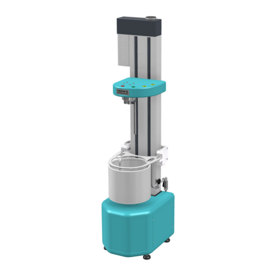
Related Manuals for Schleibinger Viskomat XL

Summary of Contents for Schleibinger Viskomat XL
- Page 1 Schleibinger Viskomat NT and Viskomat XL Schleibinger Gerte Teubert u. Greim GmbH Gewerbestrae 4 84428 Buchbach Germany Tel. +49 8086 94731-10 Fax. +49 8086 94731-14 www.schleibinger.com info@schleibinger.com April 5, 2019...
-
Page 2: Table Of Contents
2.1.1 Connecting the system ... . 2.2 Preparation for the measurement of the Viskomat NT 12 2.2.1 Installing the measuring probe ..12 2.2.2 Installing the sample container . -
Page 3: Contents
Contents 6 Plot 6.1 General information ....32 6.2 Plot area ......33 6.2.1 Title . -
Page 4: Contents
Contents 6.4.15 Line Colour ....43 6.4.16 Cut yes/no ....43 6.4.17 Cut sections . -
Page 5: Contents
13 Probe Calibration 13.1 Viskomat NT ..... . 60 13.2 The Basket Probe ....62 13.3 Viskomat XL . -
Page 6: Preface
Never open the system to try and repair it yourself - always contact the manufacturer. Protect the device from liquids. If any liquid gets into the device accidentally, unplug it and contact us. Do not try to continue using the device. Figure 1: Rheometers Viskomat NT and Viskomat XL. -
Page 7: Viskomat Operation
90 degrees. Since 2010 the silver connector is screwed to the socket (see figure 5) From 2011 a for the Viskomat NT a Lemo connector is plugged into the socket. Please don’t turn this connector, only push or pull for remov- ing (see figure 6). -
Page 8: Connectors On The Backside Of The Viskomat Elec
2 Viskomat operation Figure 2: Connectors on the backside of the Viskomat electronic Figure 3: Connectors on Viskomat NT... -
Page 9: Connectors On The Backside Of The Viskomat Xl
2 Viskomat operation Figure 4: Connectors on the backside of the Viskomat XL. Since 2011 the lift connector is beneath the motor connector. Figure 5: Connector for the Viskomat XL lift unit, used since 2010... -
Page 10: Connector For The Lift Unit, Used Since 2011
2 Viskomat operation Figure 6: Connector for the lift unit, used since 2011 Connect the electronics unit to a 110..230 V/50..60 Hz AC socket with protective earth conductor. For your own safety, make sure there is nothing standing on or rubbing against the power cable. The cooling and heating unit should not be placed in a wardrobe or cabinet because it is producing waste heat. -
Page 11: Alert Window Popping Up If The Motor Power Supply
2 Viskomat operation Figure 7: Power Switch, USB ports, status LED, version 1 Figure 8: Power Switch, USB ports, status LED, version 2 Figure 9: Alert Window popping up if the motor power supply is... -
Page 12: Preparation For The Measurement Of The Viskomat Nt
2 Viskomat operation 2.2 Preparation for the measurement of the Viskomat NT 2.2.1 Installing the measuring probe The measuring probe has a flat side at the top. Insert the probe into the sensor opening such that the flat side faces the fixing screw. -
Page 13: Fastening The Probe Into The Viskomat Nt
2 Viskomat operation Figure 10: Fastening the probe into the Viskomat NT. Don’t open this screws Tight this screw to fix the container Figure 11: Installing the sample container. -
Page 14: Position Measuring Head
2 Viskomat operation the vessel. Mount the tubes as low as possible, to avoid a collision between the measuring had and the tubes. Close the valves at the end of the tubes before you lift the tubes up, ore before you remove, to be sure that no water is lost, and no air comes into the circulation. -
Page 15: Calibrating The Torque Sensor
2 Viskomat operation 2.2.5 Calibrating the torque sensor Calibrating the gain The device is factory-calibrated at several calibration points for both measurement ranges and for clockwise and anti-clockwise rotation. This calibration is not lost during nor- mal operation, but if the torque sensor is overloaded or damaged, calibration should be repeated. -
Page 16: The Safety Guard Of The Viskomat Xl In The Working
2 Viskomat operation Figure 14: The safety guard of the viskomat XL in the working / normal position (left) and in the opened position (right). Figure 15: An alert window shows that the safety guard is open. -
Page 17: Mounting The Valves For The Double Wall Vessel For The Viskomat Xl
2 Viskomat operation Figure 16: An alert window shows that the motor power supply is off. Please close the safety guard and press ok to restart the motor power supply. 2.3.2 Mounting the valves for the double wall vessel for the Viskomat XL For cooling and heating the specimen a double wall container is used. -
Page 18: Installing The Measuring Probe
2 Viskomat operation 2.3.3 Installing the measuring probe The measuring probe has two small cylindrical rods, mounted on the upper side of the shaft of the probe. Insert the probe into the sensor opening such that the you are pulling the black star formed knob (see figure 18) to the right side of the instrument. -
Page 19: Installing And Removing The Outer Vessel
2 Viskomat operation Set the inner vessel into the outer vessel and press it into the spring loaded elements inside the outer vessel. Turn the inner vessel about 10 degrees. The sample container is now fixed in place (see figure 19). Figure 19: Installing the sample container for the Viskomat XL. -
Page 20: Position Measuring Head
2 Viskomat operation 2.3.6 Position measuring head When you start the measuring program, the measuring head au- tomatically moves to the correct position. If the device is switched off or if you want to position the measuring head, you can move it up or down by hand. 2.3.7 Calibrating the torque sensor Calibrating the gain The device is factory-calibrated at 100, 300, 500, 700, 1000, 5000 and 10000 Nmm for clockwise and... -
Page 21: Network Connection Of The Viskomat
The address is shown on the system or can be obtained from Schleibinger. The Viskomat is addressed from the control PC us- ing this address, for example with http://192.168.1.55 The network connection is best tested with the ping program. Un- der Windows, for example, you can call this via the MS-DOS shell with ping 192.168.1.55. -
Page 22: Getting Started
After approx. two minutes, a brown window is displayed containing the request for your username. Schleibinger is set as default, and should be preferred. Enter the password: viskomat. Please write the password with small caps. -
Page 23: Local Operation Of The Viskomat
2 Viskomat operation Figure 23: Main menu for operating the Viskomat NT from within the Internet browser On the left part menu bar is located. You can click any item under- lined in blue. The corresponding page will then be displayed in the right part of the window. -
Page 24: The Measuring Process
3 The measuring process Before switching off the Viskomat, exit all the programs by clicking the ’close’ icons (x). Click the red door or power switch symbol in the task bar. Click Log off. 3 The measuring process T his chapter describes the individual steps involved in taking a Viskomat measurement. - Page 25 4 Profiles For a step specification with the same values, the Viskomat will rotate at 120 rpm for 5 minutes. Enter the profile name in the next field. You can retrieve the pro- file under this name at any time and modify it or send it to the Viskomat again as a new job.
-
Page 26: Enter Profile Mask
4 Profiles constant amplitude in degrees in the 5th column of the pro- file table. Hz a-ramp = amplitude sweep: oscillation with a certain fre- quency at a fix amplitude (using step profile) or increasing amplitude (ramp profile option). You have to define the con- stant frequency in the 5th column of the profile table. -
Page 27: Enter Profile As Ramps
1 rpm, then changing to torque control, i.e. specifying a torque. The lowest speed that can be specified is 0.001 rpm, and the maximum is 300 rpm for the Viskomat NT and Geschw./Upm = Speed/rpm Zeit/min = Time/min... -
Page 28: Profile Select
4 Profiles 80 rpm for the Viskomat XL. Please note, in the case of torque control the maximum speed is about 4 rpm. Make sure that the required torque will be reached by selecting an appropriate material and measuring geometry. Also bear in mind that torque control is not infinitely fast, and that, for example, after a shear-induced breakdown, no new torque can be built up. -
Page 29: Sending The Profile To The Viskomat
4 Profiles Figure 28: File selection mask as used at several points/places in the program 4.2.1 Sending the profile to the Viskomat When you click Save and Send, the profile data is sent to the Viskomat control electronics. This takes approx. 20 seconds, dur- ing which time the status is displayed on the screen. -
Page 30: Measurement
5.1.1 Measurement Start with start button on the Viskomat The Viskomat NT has a green start button on the measurement head. By pressing this button the system automatically assigns a file name consisting of a current date and time followed by the file name extension .dat. -
Page 31: Measurement Stop
5 Measurement 5.2 Measurement Stop The measurement can be stoped at any time by pressing the red button on the measuring head of the Viskomat or by selecting the menu item Measurement Stop. By selecting the menu item Measurement Stop a confirmation is needed to make sure the measurement have to stop. -
Page 32: Plot
6 Plot 6 Plot 6.1 General information Plot allows you to display the measured data graphically in differ- ent variants. When you click this menu item, the usual file selec- tion menu is displayed. Click OK to list the measurement files. The second column contains the file name, the third column contains the associated comment. -
Page 33: Plot Area
6 Plot a hand. If you then click the x-axis, the bottom part of the window automatically scrolls to the area where you can enter the data for the x-axis. By clicking the Legend area, you can scroll to the part of the input mask where you can enter text for the legend. -
Page 34: Subtitle
6 Plot Figure 32: Input mask Plot, Plot area x- and y-axes manually. The distance between the lettering and between the grid lines must also be entered. This is done in the X-Axis and Y-Axis areas. 6.2.4 Subtitle Here you enter a subtitle to appear below the main title in a smaller font. -
Page 35: Colour/Output Type
6 Plot 6.2.6 Colour/Output Type The following options are available: Colour/JPEG An on-screen graphic is created in the JPEG for- mat. This graphic is displayed directly in the Internet browser, in colour or in grey levels. This is the default option and is supported by any Internet browser. -
Page 36: Drawing Resolution In X And Y Direction
6 Plot 6.2.8 Drawing resolution in x and y direction Here you can define the size of your sheet and thus the resolution in screen pixels. The higher the number, the higher the resolution of the graphic. However, depending on the screen resolution set, you may find that the virtual sheet is larger than the screen and so only part of the graphic is displayed. -
Page 37: Tick Spacing, Main Ticks, Small Ticks
6 Plot cylinder-cylinder probe, the basket probe or the cone-plate probe. Then you can choose as shear rate directly τ and shear stress ˙ γ . Therefore you have to select here the probe type for correct calculating the shear stress and the shear rate. If you are using other units then τ... -
Page 38: From/To
6 Plot Figure 34: Y-Axis area 6.4.1 From/to If the autoscaling function is not activated, you can select the axis section here. 6.4.2 Grid Here you can select whether or not you want a grid to be displayed in the background of the measurement. 6.4.3 Tick spacing, Y - Main ticks, Y - Small ticks As with the x-axis, here you enter the distance between the ticks and lettering on the y-axis and between the grid lines. -
Page 39: Data Set
6 Plot 6.4.7 Data set Here you select the measurement file to be assigned to the y-axis. 6.4.8 Unit Here you select which measurand of the measurement is to be represented. 6.4.9 Probe If you are working with the standard probes like the mortar or the cement paste probe you are making a relative measurement. -
Page 40: Vessel Angle Over Time, And Resulting Force On The
6 Plot The test procedure is defined within the profile see chapter 4.1. We will now focus on the frequency sweep. In the picture 35 you may see the angle of the vessel over time (black function) and the measure torque (red curve). You see that the delay between stress and strain is varying over time, also the amplitude of the strain is changing over frequency. -
Page 41: Torque Over Angle. A Typical Lissajous Figure. Ma
6 Plot Figure 36: Torque over angle. A typical Lissajous figure. Material wallpaper paste. Instrument: Viskomat XL G’’ δ G’ Figure 37: Calculation G and G from the ellipse The program is offering 4 calculations for δ, tan(δ), G and G The calculation of this parameters is not a trivial task, because most of the real materials have no linear response and are strongly time dependent. -
Page 42: Paste. Instrument: Viskomat Xl
6 Plot 2. Calculate the major and minor axis plus rotation angle. This is be done by using the inverse of the Covariance Matrix for all points of the ellipse. G is the has the length and the direction of the positive major axis. G , G δ and tan(δ) may be easily calculated from G . -
Page 43: Line Style
6 Plot 6.4.11 Line Style The usual line style is continuous lines connecting all measure- ment points. You can also use dotted and dashed lines for the representation in order to differentiate the individual curves more easily, especially in a black-and-white display. If None is selected for the line style, the measurement curve is not represented using lines but the measured values are displayed as single points. -
Page 44: Y-Axis 2
6 Plot Each curve can be cut out separately. This allows you, for exam- ple, to display several flow curves for individual cut-out ranges of a measurement. If you want to enter sections in seconds, you must enter the time as a decimal fraction. 6.5 Y-Axis 2 If you have selected more than one measurement curve, an in- put field for the y-axis will be set up for each measurement curve. -
Page 45: Legend Frame On/Off
6 Plot 6.6.1 Legend Frame on/off A frame is drawn around the legend. 6.6.2 Legend Background on/off If this is set to off the legend will be transparent, i.e. the measured values and grid lines are visible right through the measurement window. -
Page 46: Lines/Arrows
6 Plot Figure 40: Entering additional text and arrows. 6.8 Lines/Arrows To mark specific places in your measurement curve, you can draw in two lines or arrows. Altogether there are two input masks available for two lines or ar- rows. The start and end positions of the line are defined in turn by a pair of numbers from the range 0-1. -
Page 47: Text On/Off
6 Plot 6.9.1 Text on/off Activates or deactivates the text lines. 6.9.2 Char Size As with the legend text, here you can define the font size from the range 0-2. 6.9.3 Text Colour Here you define the colour of the additional text. 6.10 Footnote text Above and below the drawing area you can output an additional text. -
Page 48: Graphic In An Internet Browser
6 Plot are using Windows and you right-click the graphic, you will be of- fered options for exporting it into other programs or editing it fur- ther, e.g. Open Graphic in Microsoft Word. If you are happy with the way your drawing looks, you can go back to the input mask and save all the settings you made so that you can call them up again later. -
Page 49: Data
Viskomat data into other programs or onto other systems. 7.1 XCel The Viskomat NT program offers a new interface to Microsoft’s Ex- cel spreadsheet program. This means that data can be imported directly into this program. When you click the menu item Xcel, the file selection mask described in section 4.2 is displayed. -
Page 50: Excel Opens Automatically With The Selected Mea
Simply select the function File - Save As... in Excel. If you are working di- rectly on the Viskomat NT OpenOffice instead of Excel is opened if you double-click on a *.xls file. OpenOffice is free, available for Windows, Linux and other systems and at least as powerfull as other so called standard programms. -
Page 51: Vsc
Under this menu item you can create the file format of the Visko program for the Viskomat PC. This allows you to load measure- ments from the Viskomat NT into the Visko program for the Visko- mat PC and to compare the data. When you click this item, the familiar file selection dialog opens. -
Page 52: Database
8 Viskomat files, the Windows operating system automatically opens a file se- lection dialog. You can now save this file on your local control PC. It is best to save it in the data directory of the Visko program. Then when you start the Visko program on your evaluation PC, you can load the measurement file like a Viskomat PC file. -
Page 53: Online Display
9 Online display During measuring, a graphical and a numerical online display can be shown in the browser of the Viskomat NT. The display com- prises different optional graphics in the left part of the screen and a number of numerical displays in the right part of the screen. -
Page 54: The Sidebar
9 Online display Figure 46: Settings for the online display Figure 47: Information in the title of the online graph 9.3 The sidebar On the right bar of the online graphic you see in parallel some numerical online informations. If the measurement runs you may see the actaul measurement time, if the Viskomat is not active you see the actual time. -
Page 55: Multigraph With 8 Graphs
9 Online display Measurement time Measurement time (if test is running) (if test is running) or actual time or actual time Measurement time in % Measurement time in % of the total time of the total time status status Speed in rev. per minute Speed in rev. -
Page 56: System
You save the values you have set by clicking Submit . 10.1 Setup Here you can make some basic settings for the Viskomat NT. The top part of the input mask (see figure 51) contains the height set- tings, in which you define how far the probe is to be inserted into Warning: the sample container in increments of 0.025 mm. -
Page 57: Sampling Rate
10 System Figure 51: System settings the mortar probe, the cement paste probe, the modified cement paste probe and the basket probe the values are the same. The tau factor and gamma factor are defining the the calculation from torque and speed to shear rate and shear stress. This is only used in the plot menu for a right display of γ... -
Page 58: Filter Cut-Off Frequency
4s, each value in the new file is the mean value of the last 4s/0.1s = 40 values. 10.1.4 Filter cut-off frequency The measuring-head electronics of the Viskomat NT contain a dig- ital low-pass filter. This means that the recorded torque values of the measuring head are filtered to eliminate photoelectric noise levels or high-frequency vibrations. -
Page 59: Measurement Range
For the Viskomat XL also 3.000 Nmm and 10.000 Nmm ranges are available. Please don’t select a higher range then 500 Nmm for the Viskomat NT! 10.1.9 Temp. measurement yes/no The standard probe for cement paste or mortar has an integrated temperature sensor, which also records the temperature of the sample during measuring. -
Page 60: Probe Calibration
13 Probe Calibration 13 Probe Calibration 13.1 Viskomat NT The Viskomat NT is delivered with 2 standard probes: The so called mortar probe, designed for mortar and cement paste with a maximum aggregate size from 0..2 mm (fig. 52). The so called paste probe designed for a aggregate size from 0..0.5 mm (fig. -
Page 61: Flowcurve Of A Silicon Oil With 12.7 Pa*S Measured
Figure 54: Flowcurve of a silicon oil with 12.7 Pa*s measured with the mortar-probe of the Viskomat NT at 25.2C With the plot function you may display the torque vs. speed. With a interpolation you may calculate a viscosity as described in chapter 6.4.10. -
Page 62: The Basket Probe
N is the speed of the viskomat NT in rpm, T is the measured torque in N mm. The calibration constants are then given as fol- lows: τ... -
Page 63: Viskomat Xl
Unfortunately classical rheometer geometries like come plate or cylinder-cylinder systems doesn’t work with common building ma- terials like mortar, or fresh concrete. Therefore Schleibinger has developed a different probe design to avoid segregation and sedi- mentation of the material during the measurement. -
Page 64: Viskomat Xl
Gezeichnet Montage Betonpaddel Kontrolliert unbemasste Werkst ck- kanten DIN 6784 Norm -0,1 -0,2 Schleibinger Ger te vgr-811-06-11 Buchbach 06/11 Winkel der Flunken 45 , wg Abstr. C:\CAD-Arbeitsbereich\CAD Daten\viskomat gr\(8) paddel\vgr-811-zusammenbau-betonpaddel.idw nderungen 30.09.2015 Figure 57: Geometry and dimensions of the window- or... -
Page 65: Flowcurve Of A Silicon Oil With 12.5 Pa*S Measured
13 Probe Calibration Vskomat NT Concrete / Fishbone Probe 12.5 Pa*s 300.0 2015_Oct_5_Mon_15_51_23_fishbone_probe4.dat 250.0 2015_Oct_5_Mon_15_51_23_fishbone_probe4.dat h : 4.741 g : 0.010 korr :0.99981 2015_Oct_5_Mon_15_51_23_fishbone_probe4.dat h : -0.010 g : 25.099 korr :-0.99306 200.0 150.0 100.0 50.0 10.0 20.0 30.0 40.0 50.0 v /rpm Figure 58:... -
Page 66: Non Newtonian Fluids
NIST Several authors tried a calibration for the mortar or paste probe of the Viskomat NT. For the the mortar probe Flatt, Larosa and Rous- sel [1] tested in 2006 a polymer solution in a cp system against the Viskomat NT mortar-probe. The found the calibration coefficients shown in tabular 3. -
Page 67: The Vane Probe
13 Probe Calibration Table 4: Calibration constants from Banfill for the mortar-probe for the Viskomat NT. Attention: c seems to be wrong by factor 2 Shear rate /min 0.166 Shear stress P a/(N mm) Viscosity 1/G = c (P a s)/(N mm)(min) 46.8... - Page 68 M is the measured torque, a is the radius and l the length of the blades. For the Viskomat NT the probe has a radius a of 20 mm and a length l of 60 mm. For the Viskomat XL we have the following dimensions: l/a = 69mm/34.5mm = 2...
-
Page 69: Comparing The Vane And The Mortar Probe
13.6 Comparing the Vane and the Mortar Probe In the following graphs you may see a comparison of the mortar probe and the vane probe of the viskomat NT. The profile was simply an acceleration from 0 to 120 rpm in one minute and going back to 0 in another minute. -
Page 70: Comparison Of The Vane Probe And The Mortar Probe
References Viskomat NT 2016_16469 TU Wien 70.00 60.00 50.00 40.00 30.00 20.00 2016_Nov_20_Sun_17_12_55_500Nmm_oiltest_tu_wien.dat Mortar Probe 2016_Nov_20_Sun_17_46_55_oiltest_vane.dat Vane Probe dia. 40 mm / height 60 mm / 6 blades 10.00 0.00 0.00 50.00 100.00 150.00 200.00 v / Upm Figure 61: Comparison of the vane probe and the mortar probe with silicon oil as Newtonian fluid. -
Page 71: The Chiller Ukh
14 The Chiller UKH 67.2 For temperature control you may use the Chiller UKH 67.2. Please place the chiller near the Viskomat NT. Best position is below the Viskomat, for example below the table where the Viskomat stands. The chiller has a built in fan and needs open air circulation. So don’t place it in a closed cupboard or cabinet. -
Page 72: Chiller Inlet
14 The Chiller UKH 67.2 Figure 64: Chiller inlet. Figure 65: Chiller on/off button (red), on/off button for the cooling machine (green) and the controller. To program the set temperature please use the arrow buttons at the controller as shown in figure 65. Please set now temperatures below +5 C and for safety reasons no temperatures above +65 C. - Page 73 15 Packing List: 15 Packing List: part quantity Viskomat Electronic Connectin cables Probe cable Mortar probe Paste probe mod. Paste probe Outer Vessel Valves with screws Vessel TFT Display Keyboard Mouse Mousepad Scraper Allen key User Manual Network cable Multiple socket Mains wires Circulating unit Polysiloxane tube...
- Page 74 ......Connectors on Viskomat NT ....
- Page 75 System settings ..... 57 Geometry and dimensions of the mortar-probe for Viskomat NT..... . . 60...
- Page 76 Geometry and dimensions of the paste-probe for Viskomat NT..... . . 60 Flowcurve of a silicon oil with 12.7 Pa*s measured with the mortar-probe of the Viskomat NT at 25.2C .
Need help?
Do you have a question about the Viskomat XL and is the answer not in the manual?
Questions and answers