Page 1 ® 5330A Programmable Cross Spectrum Analyzer Operation and Service Revision 1.2a September 20, 2017...
Page 2 Manual and software copyright © 2012 Miles Design LLC. All rights reserved. TimePod® is a registered trademark of Microsemi Corporation 16430 57 Ave SE Snohomish, WA 98296 425-351-5226 www.miles.io Support: john@miles.io...
Page 3: Table Of Contents
Table of Contents Introduction ............................9 Specifications ............................11 Getting started ............................13 What’s in the box? ..........................13 Sales and technical support ....................... 13 USB driver and software installation ....................15 Front panel features .......................... 17 Rear panel features ........................... 19 Choosing an external reference ......................
Page 4 Navigating zoomed graphs ......................49 Hints for phase/frequency stability measurements ................ 51 Phase noise, AM noise, and jitter ....................... 53 Integrated noise and jitter measurement ..................54 The spur table ..........................55 Show or hide known spurs ......................55 Spur measurement options ......................56 Is it a spur, or isn’t it? ........................
Page 5 Edit Menu ............................71 Trace properties (e) ........................71 Flatten selected or zoomed phase data (Ctrl-f) ................73 Remove selected or zoomed phase data (F4) ................. 74 Subtract global linear phase trend (frequency offset) (Ctrl-o) ............75 Subtract global linear frequency trend (drift line) (Ctrl-l) ..............75 Subtract quadratic linear frequency trend (drift curve) (Ctrl-q) ............
Page 6 Edit colors ............................89 High contrast (C) ..........................89 Numeric table (Ctrl-n) ........................90 Show cursor time (Ss) ........................90 Show cursor time (Hh:Mm:Ss)......................90 Show cursor time/datestamp ......................90 Do not show cursor values ......................90 Browse plots one at a time (b) ....................... 91 Overlay all loaded plots (o) ......................
Page 7 Toggle script console for selected plot (F11) ................101 Stop all running scripts (F12) ......................101 Acquire Menu ..........................103 Miles Design TimePod ........................103 Acquire from counter in Talk-Only mode ..................103 Acquire from live ASCII file ......................104 HP 53131A/53132A/53181A ......................
Page 8 Using STREAM.EXE........................... 137 /serial:<sernum> ......................... 137 /file:<filename> ........................... 137 /logfile:<filename> ........................138 /port:<portnum> ......................... 138 /msglvl:<0-5> ..........................139 /format:<P, F, TSC> ........................139 /window:<samples>........................140 /rate:<1, 10, 100, 1000> ......................141 /timestamp:<s, MJD> ........................143 /sep:<character> ......................... 143 /ref:<Hz> ............................. 144 /input:<Hz>..........................
Page 9: Introduction
RF sources and two-port devices at frequencies from 0.5 MHz to 30 MHz. Results can be viewed at timescales ranging from femtoseconds to days. Measurements made by the TimePod 5330A include the following: Real-time ‘strip charts’ of phase and frequency differences at subpicosecond precision...
Page 11: Specifications
Specifications Input frequency and level 0.5 MHz – 30 MHz, -5 dBm - +20 dBm, 50 ohm TNC-F Reference frequency and level 0.5 MHz – 30 MHz, -5 dBm - +20 dBm, 50 ohm TNC-F Input/reference VSWR (0.5-25 MHz) 1.5:1 or better Input/reference port isolation (10 MHz) 130 dB or better Maximum allowed DC at any RF input...
Page 13: Getting Started
Getting started What’s in the box? Please check the contents of your package carefully upon arrival. Each TimePod 5330A unit should be accompanied by the following items: • (1) USB 2.0 cable, A Male / B Male • (1) Power supply •...
Page 15: Usb Driver And Software Installation
CPU with SSE2 support. A dual- or quad-core processor is strongly recommended. By default, TimeLab will automatically check the Miles Design web site on a weekly basis and inform you if a newer version is available for download. Updates are always free of charge. To configure or disable automatic update notifications, select Help→Check for...
Page 16 To perform measurements with the 5330A, an Intel Core 2 Duo or faster processor is required. Referring to the benchmarks at http://www.cpubenchmark.net/common_cpus.html, the minimum PassMark score for reliable acquisition falls in the 1,600 to 2,000 range. Use of a system with inadequate CPU performance may result in acquisition errors, often accompanied by a flashing red fault indication on the 5330A’s status LED.
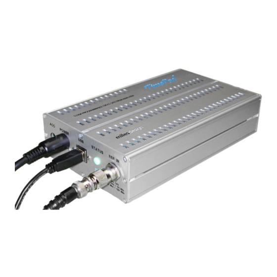
Page 17: Front Panel Features
Why the added complexity? Wouldn’t a single input jack be enough? The 5330A is really two identical instruments in one box. Each of these two “instruments” consists of a pair of software-defined HF receivers for the DUT and reference input signals. All four receiver channels are implemented with high performance 16-bit RF ADCs.
Page 19: Rear Panel Features
USB 2.0 High Speed support is required for all 5330A acquisitions. In most cases the use of passive or active USB hubs with the 5330A is acceptable, but if connection problems occur, you may find it helpful to connect the supplied USB cable directly to the host PC.
Page 20: Choosing An External Reference
Choosing an external reference In addition to the host PC and an appropriate power source, all measurements made with the 5330A require an external reference to be supplied at the REF IN jack. Virtually all aspects of measurement performance – accuracy, repeatability, noise floor, spurious responses – depend on your ability to provide the best reference signal possible.
Page 21: Making Your First Measurements
, TimeLab is not a large program, and it’s not well served by a large manual. Likewise, the TimePod 5330A hardware is easy to work with after some basic measurement concepts are understood. As an introductory exercise – or a quick operational check – you may wish to perform a measurement using the default acquisition parameters in TimeLab.
Page 22 Assuming the appropriate TimePod 5330A instrument is selected, the acquisition parameters are all valid, you’ve connected stable reference and DUT input sources to the 5330A, and you’ve allowed at Start Measurement least a few minutes’ warmup time, all you need to do is press the button.
Page 23 associated with a given measurement. This data includes the entire phase record, as well as the FFT bins from the phase noise and AM noise plots. You don’t have to wait for the measurement to end; at any time during a measurement, you can save the available data to a .TIM file or load another .TIM file for display alongside the existing plot(s) that have been loaded or acquired.
Page 24: Tips For New Users
TimeLab v1.003 (RC4) contains new versions of both files, MD5330A_100.bit and MD5330A_100.fx2. These files are present in the directory where TimeLab was installed – normally c:\Program Files\Miles Design\TimeLab. Users of TimePod 5330As prior to S/N 55985 should upgrade their hardware with both of these files, particularly if USB connectivity problems have been encountered.
Page 25 This is subject to available memory and CPU resources, of course. A typical TimePod 5330A acquisition takes about 16 MB/sec of USB bandwidth and about one core's worth of CPU horsepower.
Page 27: A Brief Architectural Note
A brief architectural note It can be helpful to understand some basic details about the TimePod 5330A’s DSP topology, especially when measurements may be constrained by available memory and CPU resources. A key observation is that each of the three basic measurement types...
Page 28 xDEV and frequency-difference plots will be recalculated, but nothing will happen to the phase noise or AM noise plots. These graphs are created by calculating phase and/or amplitude differences for all four baseband streams -- Q0,I0, Q1,I1, Q2,I2, and Q3,I3 –...
Page 29: Making Measurements
Making measurements Three views of the same TimePod 5330A measurement, in which a GPS-disciplined oscillator was used as a reference to measure a high-quality HP 10811 OCXO. The Allan Deviation plot can reveal frequency stability at timescales from milliseconds to days, while the Phase Noise plot can show you the signal’s USB...
Page 31: What's All This Adev Stuff, Anyhow
“What’s all this ADEV stuff, anyhow?” With apologies to the late Bob Pease and his editors at Electronic Design, here are a few tips to help you understand what Allan deviation (ADEV) graphs really tell you, and how to get the most out of the statistical deviation measurements made by TimeLab.
Page 32: Allan Deviation (A)
You’re fairly certain you’ll get a different result if you calculate the Allan deviation for a set of readings taken one week apart, and still another result for a series of readings taken annually. So you record at least a few data points at these intervals as well. Now you’d like to draw a graph that shows off your watch’s performance, perhaps for bragging rights at the neighborhood pub.
Page 33: Hadamard Deviation (H)
Deviation (m) will render the two noise types separately, at the timescales where they belong. As an example, here are ADEV and MDEV plots showing the residual noise of an HP 5370B time interval counter. For this test, the counter’s START input was fed with a 1-pps divider, which was driven by a 10 MHz clock that was also connected to the STOP input using an RF splitter.
Page 34: Examining Changes In Stability Over Time
Examining changes in stability over time To make basic “dynamic ADEV” measurements , refer to the help text for the Duration Run Until fields in the acquisition dialog, as well as the Trace History field. (In the TimePod dialog, Trace History is found on the Frequency Stability tab.)
Page 35: Common Artifacts In Adev And Related Measurements
Common artifacts in ADEV and related measurements High-resolution plots captured by the 5330A can reveal artifacts that don’t seem to be present when the same measurement is made by other instruments. For example, spurs due to AC power coupling or ground loops, discussed below, appear very different when acquired at high sample rates and rendered with 20 or more ADEV bins per decade.
Page 36 Additionally, beginning with version 1.1 of TimeLab, the TimePod 5330A driver can decimate the phase-difference data it acquires. Readings are collected by sampling the Output Decimation internal phase-difference data stream at a rate determined by the field in the acquisition dialog. This feature is primarily for convenience. It can be used to reduce the size of phase records generated by very long acquisitions, for example, or when high data rates must be used in order to track drifting sources.
Page 37 probably no cure besides identifying the offending source(s) and moving sensitive equipment and cables away. Ground loops are a more likely offender, since all ports on the 5330A have ground pins or shields that are bonded to the instrument’s metal enclosure. If you can identify the offending loop, you may be able to break its RF path with a coaxial balun You can also attack the source of the loop by bonding all equipment to a common ground that’s connected to the building’s power distribution network in only one place.
Page 38 Crosstalk Finally, don’t confuse power-line spurs or other sources of low-frequency interference with crosstalk. This is an insidious artifact that may be observed in high-performance measurements – or worse, may go unnoticed. When working with the 5330A, crosstalk tends to appear when the signal frequencies at the INPUT and REF IN ports are nearly the same, but not precisely.
Page 39 trace… but when the GPSDO was powered down for the magenta trace, the spurious response vanished. Likewise, as the green trace shows, replacing the RG58 input cable with an equal length of RG400 also eliminated the interference from the house standard. As can be seen, the recommendation to use double-shielded cables with the TimePod is not born of excessive caution.
Page 40: Hints For Xdev Measurements
Hints for xDEV measurements • The TimePod 5330A does not display its own measurement floor in the ADEV, MDEV, HDEV, or TDEV views. Instead, you can (and should) make residual plots for measurements that may approach the instrument floor, using similar frequencies and signal levels.
Page 41 In the example at left, two copies of the same 3600-sample .TIM file have blue been loaded. The trace was rendered with the default Threshold of 4, while the shorter magenta trace was rendered with Threshold set to 2000. Enabling Trace→Show xDEV error bars (Ctrl-e) reveals the blue...
Page 43: Working With Phase- And Frequency-Difference Traces
Working with phase- and frequency-difference traces Phase and frequency stability data acquired by TimeLab is represented internally as an array of phase- difference samples. This is true regardless of whether the data came from a frequency counter, a time- interval counter, or a direct-digital timing analyzer. (Frequency readings are converted to phase- difference samples on the basis of their deviation from the first frequency reading acquired.) In addition to the statistical measurements such as Allan deviation that TimeLab provides, “strip chart”...
Page 44: Frequency Difference (F)
discontinuities are removed by adding or subtracting the input signal’s period whenever the sample-to-sample time difference exceeds half of that period. It’s seldom necessary to refer to the original phase-difference graph except when troubleshooting configuration problems with live TI counter measurements. In most cases you should select the Measurement→Phase difference (Unwrapped) (p) view...
Page 45: How Does Timelab Measure Frequency
Phase/frequency measurements with the TimePod For TimePod 5330A users, the situation is a bit more complex. First it must be emphasized that the values on the Measurement→Frequency difference (f)
Page 46: Measurement Initialization
Start Measurement button. Refer to the figure above, taken from the Acquire→Miles Design TimePod acquisition dialog. 1) Using the nominal ADC clock frequency specified in the acquisition dialog -- typically 78.050 MHz or 76.050 MHz -- zero-crossing detectors are used to obtain a rough estimate of the signal frequencies at the INPUT and REF IN jacks.
Page 47 Some of the implications are rather subtle. For example, if you don’t enter an explicit reference frequency, the accuracy of your frequency-count chart entries will depend on how close the actual reference frequency is to the 1-kHz rounded estimate used by TimeLab.
Page 48: Examining Traces In Detail
Examining traces in detail In the example below, a crystal oscillator was measured over a 12-hour period. The Measurement→Phase difference (p) Measurement→Frequency difference (f) views appear side-by-side for comparison. Not much detail is visible in either trace. Some sporadic frequency jumps are present, but they’re not easily examined since their height is such a small fraction of the plot’s overall magnitude.
Page 49: Navigating Zoomed Graphs
Essentially, Subtract global linear frequency trend (drift line) (Ctrl-l) removes the quadratic trend from the phase record, which has the effect of removing the linear trend from the frequency-difference plot. But there’s still an arbitrary offset in the frequency-difference view that’s forcing the Y-axis scale to +/- 1E-9, and the artifacts we’d like to examine are much smaller than this.
Page 50 In this case, though, unlocking the Y axis and drawing a box requires a lot of user interaction. Worse, you’ll end up with an “unfriendly” Y-axis scale whose random- looking values make the graph difficult to interpret. Once again, Trace→Phase/frequency traces begin at zero (z) offers a better alternative with a single keystroke: To sum up, selecting...
Page 51: Hints For Phase/Frequency Stability Measurements
Hints for phase/frequency stability measurements • Due to slight variations in FPGA/USB interface temperature that occur when acquisition begins, the 5330A’s own impact on critical residual-phase measurements can be minimized Acquire→Enable deferred acquisition (ctrl-d) if you use to force the acquisition to throw away incoming data until you press Enter to 'trigger' it.
Page 53: Phase Noise, Am Noise, And Jitter
Thanks to the magic of cross-spectrum averaging, the TimePod 5330A can measure phase noise and AM noise on HF signals at exceptionally low levels. Below are some guidelines to help you make the most of...
Page 54: Integrated Noise And Jitter Measurement
Integrated noise and jitter measurement You can display various measures of integrated phase noise between two arbitrary offsets by enabling any or all of the following Legend menu fields: Residual FM  RMS Integrated Noise (Degs)  RMS Integrated Noise (Rads) ...
Page 55: The Spur Table
The spur table The spur table is a list of all coherent amplitude- or phase-modulated spectral components detected by the instrument in the course of measuring AM noise or phase noise, respectively. Each plot acquired from an instrument that supports spur detection has its own spur table.
Page 56: Spur Measurement Options
Spur measurement options Noise and Jitter tab in the TimePod 5330A’s acquisition dialog contains two parameters that influence how spurs are recognized and recorded. First, the Spur Threshold field defines the amplitude level, relative to the average level of nearby FFT bins, below which a given bin’s amplitude will not be considered...
Page 57: Is It A Spur, Or Isn't It
Is it a spur, or isn’t it? Identifying genuine spurs while disregarding false ones can be a challenge. The 5330A’s DSP software may fail to detect spurs when they occur in clusters near the FFT segment’s resolution limits, in steeply-sloped areas of the noise trace, or near segment boundaries.
Page 58 At left, the phase noise of a very high quality crystal oscillator has been measured over the course of several hours. Most of the visible spurs are well below the 5330A’s specified limits, so it isn’t clear which ones the instrument may be responsible for. However, because complex signals are used throughout the 5330A’s DSP pipeline, we can take advantage of a mathematical observation.
Page 59: Hints For Noise Measurements
(Trace→Smooth noise traces (ctrl-w)) but it’s often not needed with a cross-correlating analyzer such as a TimePod 5330A or a TSC 5120A/5125A. The best way to obtain a smoother trace with these instruments is to let your measurement run longer. Low-level residual plots can benefit from Trace→Smooth noise traces...
Page 61: Timelab Command Reference
TimeLab command reference Most of the menu-based commands in TimeLab also have single-key shortcuts for faster, more interactive workflow. When present, the shortcut key is shown after the name of the menu option.
Page 63: File Menu
File menu The File menu helps you work with data files and images. Supported actions include opening, saving, closing, and deleting plots stored in .TIM files, saving image files, printing or copying the currently displayed window contents, and importing and exporting raw measurement data. Various “user preference”...
Page 64: Copy Image To Clipboard (Ctrl-C)
Copy image to clipboard (Ctrl-c) This command offers a handy shortcut for cutting/pasting TimeLab screen images into other programs via the operating system’s clipboard, avoiding the need to save an image file. When copying the screen image to the clipboard, all visible status and error messages, notifications, prompts, and mouse-cursor query values are removed.
Page 65: Export Ascii Phase Data (X)
Export ASCII phase data (x) This command is supported only when viewing the selected plot’s phase record contents using Measurement→Phase difference (p) Measurement→Frequency- difference (f). It will save an ASCII text file containing phase difference data in seconds, one entry per line, at 16 digits of precision to the right of the decimal point. If a selected or zoomed area has been defined by dragging with the mouse, only that portion of the phase record will be exported.
Page 66: Export Binary Phase Data
Export binary phase data This command is supported only when viewing the selected plot’s phase record contents using Measurement→Phase difference (p) Measurement→Frequency- difference (f). It will save a binary file containing phase difference data in seconds, represented as a block of double-precision IEEE 754 values in little-endian (Intel) format. If a selected or zoomed area has been defined by dragging with the mouse, only that portion of the phase record will be exported.
Page 67: Export Xdev Trace
Export xDEV trace Available in the Measurement→Allan Deviation (a), Measurement→Modified Allan Deviation (m), Measurement→Hadamard Deviation (h), Measurement→Time views, this command creates an ASCII text file containing a tau, sigma(tau) Deviation (t) value pair for each visible xDEV bin in the selected plot. One value pair is written per line;...
Page 68: Print Image
.INI files varies depending on the operating system version. In Windows 7, these files are normally located at c:\Users\<user name>\AppData\Local\Miles Design\TimeLab, also accessible at %LOCALAPPDATA%\Miles Design\TimeLab. In Windows XP, the .INI files are normally located in the hidden directory c:\Documents and Settings\<user name>\Local Settings\Application Data\Miles Design\TimeLab.
Page 69: Close All Visible Plots (Home)
.INI files varies depending on the operating system version. In Windows 7, these files are normally located at c:\Users\<user name>\AppData\Local\Miles Design\TimeLab, also accessible at %LOCALAPPDATA%\Miles Design\TimeLab. In Windows XP, the .INI files are normally located in the hidden directory c:\Documents and Settings\<user name>\Local Settings\Application Data\Miles Design\TimeLab.
Page 71: Edit Menu
Edit Menu Plots that have been loaded or acquired in TimeLab may be displayed with a variety of options and transforms. However, any changes to the measurement data or display parameters associated with a specific plot must be made through the commands in the Edit menu. Trace properties (e) Edit→Trace properties (e) As seen above, the...
Page 73: Flatten Selected Or Zoomed Phase Data (Ctrl-F)
Flatten selected or zoomed phase data (Ctrl-f) Above, the Flatten selected or zoomed phase data (Ctrl-f) command has replaced the selected region of the phase record with a straight line. The result appears as a flat spot in the Frequency Difference measurement view. This command is supported only when viewing the selected plot’s phase-record Measurement→Phase difference (p) Measurement→Frequency-...
Page 74: Remove Selected Or Zoomed Phase Data (F4)
Remove selected or zoomed phase data (F4) Like Edit→flatten selected or zoomed phase data (Ctrl-f), this command is useful for removing glitches and outliers from the selected plot’s phase record. Instead of replacing the affected region with a straight line, however, Edit→Remove selected or zoomed phase data (F4) shortens the phase record by removing the data altogether.
Page 75: Subtract Global Linear Phase Trend (Frequency Offset) (Ctrl-O)
Subtract global linear phase trend (frequency offset) (Ctrl-o) Subtract global linear frequency trend (drift line) (Ctrl-l) Subtract quadratic linear frequency trend (drift curve) (Ctrl-q) These related commands are used to remove global offsets and trends from the selected plot’s phase record. This is typically done to improve visibility of local trends and features whose magnitude is small compared to the Y-axis range.
Page 77: Trace Menu
Trace Menu Trace menu contains options that affect the way measurement data is processed and rendered as traces on the graph. Unlike the Edit menu options, the Trace options apply to all visible traces, rather than only the selected plot, and they never alter the underlying measurement data. Most options on the Trace menu apply only to a given measurement family –...
Page 78 When used in the Measurement→Frequency difference (f) view, the effect of Trace→Phase/frequency traces begin at zero (z) is somewhat similar to applying Edit→Subtract global linear phase trend (frequency offset) (Ctrl-o) to each visible plot. It’s not quite the same, though, because a trace’s first data point is not necessarily anywhere near its trend line.
Page 79: Show Linear Phase/Frequency Trend (Ctrl-T)
detail while preserving the graph’s original shape, while is better at revealing short- term noise and other effects that become harder to spot as the graph expands to accommodate a larger overall trend. Some additional usage examples can be found on page 48. Show linear phase/frequency trend (Ctrl-t) When enabled, this option causes TimeLab to display a dashed line on unzoomed phase- and frequency-difference traces to indicate the data’s linear trend.
Page 80: Phase/Frequency Y Axis Unlocked In Zoom Mode (Y)
Phase/frequency Y axis unlocked in zoom mode (y) By default, the Y axis in phase- and frequency-difference measurement graphs is automatically scaled to accommodate the largest absolute value in all visible traces. The peak magnitude is rounded up to the next decade, half decade, or quarter decade, then mirrored to place zero at center scale.
Page 81 Warning: Averaging introduces time lag which may cause unexpected results with some commands and display options. It’s recommend that averaging be disabled before selecting regions of the phase record for any operations, or when evaluating absolute phase differences or frequency differences. At long averaging times, a substantial baseline offset can exist between the beginning and end of the trace, since there’s less historical data to contribute to the average near the beginning of the record.
Page 82: Draw Xdev Traces With Spline Interpolation (I)
Draw xDEV traces with spline interpolation (i) By default, screenspace points corresponding to the tau bins in Allan deviation and related statistical views are connected with a cubic spline. Spline interpolation results in a smooth, visually-appealing curve, but it can distort or exaggerate ringing artifacts and Trace→Draw xDEV traces with spline other abrupt transitions in the graph.
Page 83: Clip Xdev Traces By Noise Bandwidth (Ctrl-B)
Intended primarily as a diagnostic aid, this option is supported when viewing phase noise or AM noise plots from instruments such as the TimePod 5330A that support real- time cross correlation. When enabled, the FFT segments in the selected phase noise or AM noise plot will be color-coded for identification.
Page 84: Show Imaginary Part Of Cross Spectrum (Ctrl-F3)
Show imaginary part of cross spectrum (Ctrl-F3) Show estimated instrument noise (F2) Phase noise and AM noise plots acquired with the TimePod 5330A and Symmetricom 512X analyzers can be displayed with a shaded area that provides an estimate of the instrument noise floor, if you enable Trace→Show estimated instrument noise...
Page 85: Mark Spurs In Noise Traces (Ctrl-M)
(Ctrl-s) command is used to toggle spur attenuation. To obtain a smoother trace with cross-correlating analyzers such as the TimePod 5330A and Symmetricom 512x models, it’s often better to let the measurement run longer. As the trace converges on the true noise level its variance will diminish, resulting in a more accurate measurement with less visible “grass.”...
Page 86: Show Am Noise In Pn View (F8)
Show AM noise in PN view (F8) When enabled, this command renders a copy of the AM noise trace in the Measurement→Phase noise (P) view, using a lighter color or trace weight. Both PM and AM spur tables are displayed, space permitting. Tick marks (k) This command toggles tick marks on and off.
Page 87: Toggle Trace Thickness For Current Measurement (T)
Toggle trace thickness for current measurement (T) This command switches between heavy and light traces in the currently-active measurement view. TimeLab keeps track of the requested trace thickness for each Measurement menu entry.
Page 89: Display Menu
Display Menu Display-related options that aren’t measurement-specific appear on the Display menu. Controls on this menu determine the visibility and selection status of loaded plots, the order in which plots appear in the legend table below the graph, and the choice of Display→Overlay (o) Display→Browse (b) mode that...
Page 90: Numeric Table (Ctrl-N)
Numeric table (Ctrl-n) The numeric table appears to the right of the graph area in each measurement view, unless toggled off with this command. The format of the table is different for each measurement type. In the Allan deviation and other statistical views, a chart displays the sigma(tau) values at assorted tau intervals.
Page 91: Browse Plots One At A Time (B)
Browse plots one at a time (b) Overlay all loaded plots (o) Toggle visibility of selected plot (v) Since TimeLab allows up to nine plots to be loaded and displayed at once, these three commands are needed to maintain a legible display. They are often used together in rapid succession, so they will be described together and referenced in abbreviated form.
Page 92: Zoom In ( ] )
X zoom in ( ] ) X zoom out ( [ ) Y zoom in ( } ) Y zoom out ( { ) The bracket and shift-bracket keys are useful for navigating zoomed phase- and frequency-difference traces on a laptop or other PC without a three-button scrolling mouse.
Page 93: Legend Menu
Legend Menu Legend menu determines which attributes are displayed for each visible plot in the legend table beneath the main graph. Some properties are flagged for display in the legend table by default, while others will not be displayed until you select them in the Legend menu.
Page 94 Imported From Name of file or device from which data was imported Incoming Sample Interval Time in seconds between successive data points from the instrument Input Amplitude Approximate input amplitude in dBm Input Estimated True if input frequency is a low-precision estimate that should be rounded for display Input Freq Input frequency Input Splitter...
Page 95: Measurement Menu
As discussed on page 27, TimeLab plots (and their associated .TIM files) use independent data records for different measurement classes. Some instruments like the TimePod 5330A can acquire data for all measurements supported by TimeLab, but most are limited to specific measurement types. For...
Page 97: Masks Menu
Masks Menu menu is almost entirely user-configurable. It consists of a list of mask definitions for optional Masks use in TimeLab. Masks are useful in production test applications where fast, reliable, and repeatable pass/fail judgments are required. You can also use mask testing for proof-of-performance verification of the TimePod and other instruments supported by TimeLab.
Page 98: Edit Mask Definitions
For detailed instructions and hints, carefully review the comments in masks.txt. The latest usage guidelines for the current TimeLab release will appear as comments in this file. Edit mask definitions . . . As noted above, the last command on the Masks menu opens masks.txt in Notepad for editing and review.
Page 99: Scripts Menu
Save measurement script. They exercise virtually all of the capabilities of the TimeLab script API as well as those of the TimePod 5330A itself. By default, script files are stored in the %ALLUSERSPROFILE%\Documents\TimeLab\Scripts folder. This folder’s location will vary from one Windows version to the next. For example, in a typical Windows 7...
Page 100: Run Script
Run script … To launch a test script, select Scripts→Run script . . . and choose the desired script’s JavaScript file (.js) in the file dialog that appears. TimeLab will load the script into memory and execute its “global scope” to initialize any variables declared outside of functions or event handlers.
Page 101: Toggle Script Console For Selected Plot (F11)
Toggle script console for selected plot (F11) When a measurement is started under script control, TimeLab will display an overlay containing any error or status messages issued by the script. This console overlay is shown by default whenever the measurement is otherwise visible on the graph.
Page 103: Acquire Menu
Acquire Menu TimeLab’s principal mission is to serve as the user interface for the TimePod® 5330A Programmable Cross Spectrum Analyzer from Miles Design, but support for many other instruments is also provided. Acquire menu includes a list of all instruments recognized by TimeLab, followed by a small number of commands that manage acquisition operations.
Page 104: Acquire From Live Ascii File
Acquire from live ASCII file Similar to the Talk-Only acquisition option described above, this option allows you to specify the location of a text file containing frequency, phase/TI, or timestamp data that’s being written by another process. TimeLab will open the file in read-only mode, process all existing data in the file if requested, and then continue to fetch data until the acquisition terminates.
Page 105: Symmetricom 5115A / 5120A / 5125A (Frequency Stability)
Symmetricom 5115A / 5120A / 5125A (Frequency stability) Symmetricom 5115A / 5120A / 5125A (Phase noise) These digital phase noise analyzers provide advanced features and specifications similar to the TimePod 5330A. However, separate options in the Acquisition menu must be used to obtain data for xDEV and phase/frequency-difference plots and the Fourier spectrum used for phase noise plots.
Page 106: Abort And Retrigger Selected Acquisition (Ctrl-A)
Abort and retrigger selected acquisition (Ctrl-a) Keep and retrigger selected acquisition (Ctrl-k) Like Acquire→Stop/repeat acquisition (Space) , these commands are normally accessed via their respective keyboard shortcuts. Often used when you accidentally disturb the equipment or remember an omitted step in the measurement procedure, Ctrl-a will restart the selected plot’s measurement immediately with no further interaction.
Page 107: Enable Deferred Acquisition (Ctrl-D)
When making deferred measurements with the TimePod 5330A, you should consider using scripting techniques instead, as demonstrated in the OCXO_2hr_stability_test.js example. Because the 5330A will not tolerate excessive DUT drift while waiting for a deferred measurement to begin, OCXO_2hr_stability_test.js delays the entire...
Page 109: Help Menu
TimeLab and access the latest edition of the TimePod 5330A Operation and Service manual (this file). When you install TimeLab, a local copy of the TimePod 5330A manual is also installed on your hard drive.
Page 111: Appendix: Some Examples Of Residual Performance
Appendix: Some examples of residual performance The gold-standard diagnostic resource for the TimePod 5330A is a simple residual test, conducted after at least a 1-hour warmup, in which you drive the inputs at >= 10 dBm using a clean signal (i.e., without excessive broadband noise) fed through a passive splitter (Mini-Circuits ZFSC-2-1 or similar).
Page 112 Despite visible HVAC cycling, overall phase stability is within +/- 1 ps over the entire 12-hour 5 MHz run. The 25 MHz residual trace, on the other hand, was taken with inadequate warmup time. It begins with about 30 minutes of noticeable phase drift (about three picoseconds) until the TimePod’s internal components reach thermal equilibrium.
Page 113 As expected, residual phase noise performance is improved when a strong 5 MHz signal is measured for hours, compared to a weaker 25 MHz signal measured for 3 hours. The difference in AM noise isn’t as pronounced in this case.
Page 115: Appendix: Javascript Api Function Reference
TimeLab includes an embedded JavaScript engine that can run automated test scripts using the TimePod 5330A. (Script-based access to other instruments such as time-interval counters is not currently supported.) The API functions listed below are useful in a variety of applications ranging from the standard TimePod performance verification procedures to user-developed test scripts.
Page 116 AcqGetAMSpurTable(Array offset_array, Array amplitude_array) Populates with a list of all detected AM spurs in the offset_array amplitude_array current measurement, returning the total number of AM spurs. AcqGetPMSpurTable(Array offset_array, Array amplitude_array) Populates with a list of all detected PM spurs in the offset_array amplitude_array current measurement, returning the total number of PM spurs.
Page 117 AcqParam(String key) Each script instance maintains a dictionary of acquisition parameters that can be used to override any or all of the default acquisition dialog parameters when AcqStartAcquisition() is called. returns the value for the specified acquisition parameter. AcqParam() If an existing plot is associated with the script instance, will return the specific AcqParam() value associated with the plot.
Page 118 Acquire menu, including any ellipsis (...) that follows it. Currently the only officially- supported instrument name for scripted measurements is the Miles Design TimePod ... entry, so this string should be supplied as the value. menu_entry With a script-initiated measurement, the acquisition parameters are recalled from the same driver-specific .INI file that provides the dialog defaults when the acquisition is...
Page 119 DisplayOverlayMode([Boolean overlay_mode]) Equivalent to the Display→Browse plots one at a time (b) Display→Overlay all loaded plots (o) command, depending on the parameter. overlay_mode is optional; if it is not provided by the script, the function simply returns overlay_mode true in Overlay mode or false in Browse...
Page 120 EventAcqTriggered() This is an optional user-supplied function. is called when a EventAcqTriggered() measurement initiated by begins collecting data. Typically this AcqStartAcquisition() happens a few seconds after is called by the user-provided AcqStartAcquisition() function, unless the deferred acquisition options on the Acquire menu EventRunScript()
Page 121 FileCloseAllPlots() Equivalent to calling on all loaded plots. For example, 5330A_ADC_test.js FileClosePlot() uses to ensure that enough slots are available in the legend table to hold FileCloseAllPlots() the four plots that it acquires for various ADC combinations. FileClosePlot([Number selection]) If the optional parameter is specified, closes the plot at the selection...
Page 122 FileNumUnsavedPlots() Returns the number of currently-loaded plots, from 0 to 9, that have not been saved since being acquired or modified. FileSave(String path, [String subdir,] String filename) Based on the (case-insensitive) suffix of saves either a screen image in filename FileSave() .TGA, .GIF, .BMP, .PCX, or .PNG format, or a .TIM file representing the measurement currently associated with the script.
Page 123 parameters, which will show ( ==true) or hide ( ==false) the specified status status field_name in the table and return its previous state. MaskResultMargin() Returns a Number value representing the margin by which the measurement associated with the script is passing (if positive) or failing (if negative) the mask test selected by The returned value is based on the most recently rendered frame, so it is MaskSelect().
Page 124 MaskSelect([String mask_name]) This function selects a mask for use with , returning MaskResultMargin() MaskResultValid() the previously-selected mask if any. If is omitted, the function returns the mask_name currently-selected mask name. In both cases, the function will return an empty string if no mask was selected.
Page 125 When a measurement initiated by a script specifies multiple stability channels, as in the TimePod 5330A validation scripts mentioned, it’s necessary to use ScriptBindToPlot() access the plots that represent all channels of the measurement.
Page 126 ScriptEnd() Marks the script for cleanup by the TimeLab runtime JavaScript engine. Scripts which are associated with loaded plots must be terminated with a call to when ScriptEnd() finished. Otherwise, they will continue to run (and consume resources) until one of the following conditions is true: - A script exception or other fatal error occurs - The...
Page 127 ScriptGetString(String heading, String message, Object user_text, String b1_text [, String b2_text [, String b3_txt]]) Presents a modal dialog box to the user that accepts freeform text entry. An example appears below. var trace_caption = { value:"(Some default text could go here)" }; if (ScriptGetString( "OCXO Stability Test", "Enter trace caption above, then click 'OK' to continue.",...
Page 128 ScriptMessageBox(String heading, String message, String b1_text [, String b2_text [, String b3_txt]]) Presents a modal dialog box to the user that accepts button presses. An example appears below. if (ScriptMessageBox( "Manufacturing Test", "Connect input signals and click 'OK' to continue.", "OK", "Cancel") != 0) ScriptEnd();...
Page 129 ScriptNumVal(String format_string, Number value) Returns a String consisting of the specified with an embedded numeric format_string value. In operation, passes its and floating-point arguments to ScriptNumVal() format_string value the standard C sprintf() function, returning the resulting formatted string. Example: The following statement Print(ScriptNumVal("Pi = %.2lf", 3.1415926535));...
Page 130 ScriptShowTTY([Boolean show]) Shows or hides the script TTY window that is associated with the plot(s) bound to the script instance, returning the previous visibility state. If the argument is omitted, show the function will return the current visibility state without changing it. The script TTY window becomes visible by default upon successful execution of .
Page 131 TimeSetTimer(Number msec) This function arranges for TimeLab to call the script’s handler at regular EventTimer() intervals of milliseconds. msec Because TimeLab’s scripting system relies on cooperative multitasking, most non-trivial scripts should carry out the majority of their processing work in their handler EventTimer() while their measurement(s) are in progress.
Page 132 TracePhaseFreqResid([Boolean status]) Sets and/or retrieves the of the flag controlled by Trace→Show linear status phase/frequency residual (r). Refer to this command for more information. To return the current flag value, call with no argument. TracePhaseFreqResid() TracePhaseFreqTrend([Boolean status]) Trace→Show linear Sets and/or retrieves the of the flag controlled by status phase/frequency trend...
Page 133 TraceShowSlopes([Boolean status]) Sets and/or retrieves the of the flag controlled by Trace→Show FFT segment filter status slope(s) (Ctrl-i). Refer to this command for more information. To return the current flag value, call with no argument. TraceShowSlopes() TraceSmoothNoise([Boolean status]) Trace→Smooth noise traces Sets and/or retrieves the of the flag controlled by status...
Page 134 TraceXDEVSpline([Boolean status]) Sets and/or retrieves the of the flag controlled by Trace→Draw xDEV traces with status spline interpolation (i). Refer to this command for more information. To return the current flag value, call with no argument. TraceXDEVSpline()
Page 135: Appendix: The Stream.exe Phase/Frequency Data Server
TimeLab includes a Windows console application, STREAM.EXE, which can be used to provide remote access to measurement data acquired by a TimePod 5330A. Continuous streams of phase-difference or frequency measurements acquired by STREAM.EXE can be written to a shared file or streamed...
Page 136: Launching Stream.exe
DOS session and changing the current directory to c:\Program Files\Miles Design\TimeLab. To do this, select Start → Run… in Windows and enter cmd as the name of the program to run. Once the DOS box appears, drag its lower edge to expand the window to a more comfortable size.
Page 137: Using Stream.exe
Using STREAM.EXE Because STREAM.EXE performs only phase/frequency stability measurements, its command-line options are relatively limited. Only one parameter is mandatory: you must specify the hardware driver’s filename as the first parameter on the command line. Currently, only the TimePod driver is supported, so all STREAM.EXE command lines must begin as follows: stream timepod.tll Additional options, described below, may be specified as needed.
Page 138: Logfile:
Additionally, the /notcp option Is used in this example to keep STREAM.EXE from attempting to open a network port. /logfile:<filename> Specifies the pathname for a logfile which will record status, warning, and error messages. If the /logfile parameter contains an absolute path specification, the log file is placed at that location.

Page 139: Msglvl:<0-5
/msglvl:<0-5> Specifies the “verbosity” of informational, warning, and error messages that STREAM.EXE will display on the server console. /msglvl:0 will display all available status messages and notices, including internal driver diagnostic messages, while /msglvl:5 will display only fatal error messages. The default message level is 3. Messages displayed at the server console are also written to the logfile.
Page 140: Window:
client(s) by STREAM.EXE for display in their status lines. In /format:TSC mode only the numeric phase data is transmitted, for compatibility reasons. See the /input and /ref descriptions below for important additional notes. /window:<samples> When the /format:F option is used to acquire a stream of absolute frequency measurements, each frequency reading is normally derived by subtracting the previous phase-difference reading from each incoming one and dividing the result by the reciprocal of the sampling interval.

Page 141: Rate:<1, 10, 100, 1000
Here, the frequency readings in green were displayed by turning Scroll Lock on to view the data in real time as it was acquired. After only 24 seconds, the results have converged to within about 3 parts in 10 of the expected value of 9999999.962747097 MHz.
Page 142 measurements of drift-prone sources may require /rate:100 or /rate:1000 to avoid acquisition failures. Note that measurements made at 1 reading per second are likely to fail if insufficient warmup time is allowed for the DUT, the reference source, or the TimePod itself.
Page 143: Timestamp:
/timestamp:<s, MJD> /sep:<character> These related options cause STREAM.EXE to timestamp each phase-difference or frequency reading sent to files or network clients. By default, no timestamps are emitted. When /timestamp:MJD is specified, the Modified Julian Date (MJD) associated with each phase-difference or frequency value will be written as the first numeric field on each line, followed by a space character (ASCII 32), then the measurement value itself.

Page 144: Ref:
/ref:<Hz> /input:<Hz> When acquiring data directly from a TimePod, TimeLab rounds its reference and input frequency estimates according to the process described on pages 43-45 (“Phase/frequency measurements with the TimePod”). The TimeLab acquisition dialog also allows you to enter explicit input and reference frequencies if desired. As explained in that section of the manual, the reference-rounding process provides the best achievable frequency count chart accuracy when highly-accurate references are in use, while the ability to enter explicit input and reference frequencies allows you to make...

Page 145: Autoupdate
/autoupdate The /autoupdate function is useful in scenarios where STREAM.EXE may need to be recompiled, upgraded, or otherwise replaced over a network without manual intervention at the server console. When /autoupdate is present on the command line, STREAM.EXE will periodically check for the presence of a file called STREAM.EX1 in the same directory as the executable.
Page 146: Noexit
/noexit By default, STREAM.EXE will disconnect any attached clients, close its destination file (if any), and terminate with exit(1) under a variety of abnormal conditions, including loss of input or reference signals, out-of-range signal frequencies or amplitude levels, or other acquisition errors.
Page 147: Appendix: Schematic Diagrams And Service Notes
Appendix: Schematic diagrams and service notes The TimePod® 5330A’s FPGA constraints file, timepod.ucf, is supplied in the drivers/TimePod subdirectory beneath the TimeLab installation folder. The USB interface API and Cypress FX2LP microcontroller source code is also supplied in XEM3005.zip. These resources are provided under the terms of the TimeLab software license (page 157) to support the development of custom measurement applications with the TimePod hardware.
Page 155: Appendix: Legal And Regulatory Notices
Appendix: Legal and regulatory notices...
Page 156: Federal Communications Commission Statement
Changes or modifications not expressly approved by the party responsible for compliance may void the user's authority to operate the equipment. EC Declaration of Conformity Manufacturer: Miles Design LLC, 16758 45 Ave NE, Lake Forest Park, Washington 98155 USA Product: MD 5330A Programmable Cross Spectrum Analyzer...
Page 157: Performance Certification And Validation
Miles Design LLC warrants the TimePod® 5330A Programmable Cross Spectrum Analyzer against all defects in materials and workmanship for a period of ONE (1) year from the date of original customer delivery. The sole responsibility of Miles Design LLC under this Warranty is limited to repair or replacement of the TimePod® 5330A Programmable Cross Spectrum Analyzer, at the sole discretion of Miles Design LLC.
Page 158: Software License: Fftss
Software License: FFTSS http://www.ssisc.org/fftss/index.html.en Copyright 2002-2007 Akira Nukada. All rights reserved. Copyright 2002-2007 The SSI Project. All rights reserved. The Scalable Infrastructure Project, supported by "Development of Software Infrastructure for Large Scale Scientific Simulation" Team, CREST, JST. Akira Nishida, Department of Computer Science, The University of Tokyo, 7-3-1 Hongo, Bunkyo-ku, Tokyo 113-8656, Japan. Redistribution and use in source and binary forms, with or without modification, are permitted provided that the following conditions are met: Redistributions of source code must retain the above copyright notice, this list of conditions and the following...
Page 159 receive source code or can get it if you want it; that you can change the software and use pieces of it in new free programs; and that you are informed that you can do these things. To protect your rights, we need to make restrictions that forbid distributors to deny you these rights or to ask you to surrender these rights.
Page 160 or a portion of it, either verbatim or with modifications and/or translated straightforwardly into another language. (Hereinafter, translation is included without limitation in the term "modification".) "Source code" for a work means the preferred form of the work for making modifications to it. For a library, complete source code means all the source code for all modules it contains, plus any associated interface definition files, plus the scripts used to control compilation and installation of the library.
Page 161 If distribution of object code is made by offering access to copy from a designated place, then offering equivalent access to copy the source code from the same place satisfies the requirement to distribute the source code, even though third parties are not compelled to copy the source along with the object code.
Page 162 a) Accompany the combined library with a copy of the same work based on the Library, uncombined with any other library facilities. This must be distributed under the terms of the Sections above. b) Give prominent notice with the combined library of the fact that part of it is a work based on the Library, and explaining where to find the accompanying uncombined form of the same work.
Page 163: Software License: V8 Javascript Engine
NO WARRANTY 15. BECAUSE THE LIBRARY IS LICENSED FREE OF CHARGE, THERE IS NO WARRANTY FOR THE LIBRARY, TO THE EXTENT PERMITTED BY APPLICABLE LAW. EXCEPT WHEN OTHERWISE STATED IN WRITING THE COPYRIGHT HOLDERS AND/OR OTHER PARTIES PROVIDE THE LIBRARY "AS IS" WITHOUT WARRANTY OF ANY KIND, EITHER EXPRESSED OR IMPLIED, INCLUDING, BUT NOT LIMITED TO, THE IMPLIED WARRANTIES OF MERCHANTABILITY AND FITNESS FOR A PARTICULAR PURPOSE.