
Related Manuals for Hioki 8847

Summary of Contents for Hioki 8847
- Page 1 Instruction Manual 8847 MEMORY HiCORDER December 2010 Revised edition 4 8847A981-04 10-12H...
-
Page 3: Table Of Contents
Contents Contents Usage Index ................1 Introduction.................2 Confirming Package Contents............2 Safety Information ..............3 Operating Precautions..............6 Chapter 1 Overview ___________________________________ 9 Product Overview ..............9 Names and Functions of Parts .......... 10 Screen Organization ............12 Basic Key Operations ............14 1.4.1 Example for Using the HELP Key ...........15 Chapter 2 Measurement Preparations___________________ 17 Install an input module ............ - Page 4 Contents Setting Measurement Configuration ......... 41 3.4.1 Measurement Function ............41 3.4.2 Time Axis Range and Sampling Rate ........43 3.4.3 Recording Length (number of divisions) ........ 46 3.4.4 Screen Layout ................ 48 Input Channel Setting ............49 3.5.1 Channel Setting Workflow ............50 3.5.2 Analog Channel ..............
- Page 5 Contents Chapter 6 Printing ___________________________________ 89 Printing Type and Workflow ..........90 Making Auto Print Settings ..........91 Manual Printing With PRINT key (Selective Printing) ..93 Setting the Print Concentration of the Waveform ....94 Making Printer Settings ............. 95 Miscellaneous Printing Functions ........98 6.6.1 Screen Hard Copy ..............98 6.6.2...
- Page 6 Contents Displaying Waveforms During Recording (Roll Mode) ... 124 Displaying New Waveforms Over Past Waveforms (Overlay) ................. 125 Setting Channels to Use (Extending the Recording Length) ........127 Converting Input Values (Scaling Function) ....128 8.5.1 Scaling Setting Examples ............ 130 Variable Function (Setting the Waveform Display Freely) 134 Fine Adjustment of Input Values (Vernier Function) ..
- Page 7 Contents Chapter 10 Numerical Calculation Functions _____________ 173 10.1 Numerical Calculation Workflow ........174 10.2 Settings for Numerical Value Calculation ......176 10.2.1 Displaying Numerical Calculation Results ......179 10.3 Judging Calculation Results ..........180 10.3.1 Display of Judgment Results and Signal Output ....182 10.4 Saving Numerical Calculation Results ......
- Page 8 Contents 13.3.8 Emphasizing Analysis Results (phase spectra only) ... 219 13.3.9 Analysis Mode Settings ............220 13.3.10Setting the Display Range of the Vertical Axis (Scaling) ..224 13.3.11Setting and Changing Analysis Conditions on the Waveform Screen ............. 225 13.4 Selecting Channels ............226 13.5 Setting Screen Displays ..........
- Page 9 Contents 15.7 Controlling the Instrument with Command Communications (LAN/USB) ..............282 15.7.1 Making Settings on the Instrument ........283 15.7.2 Communication Command Setting ........284 Chapter 16 External Control ___________________________ 287 16.1 Connecting External Control Terminals ......288 16.2 External I/O ..............289 16.2.1 External Input (START/EXT.IN1) (STOP/EXT.IN2) (PRINT/EXT.IN3) ..............289 16.2.2 External Output (GO/EXT.OUT1) (NG/EXT.OUT2) ....290 16.2.3 External Sampling (EXT.SMPL) ...........291...
- Page 10 viii Contents 18.2 Initializing the Instrument ..........314 18.2.1 Initializing System Settings (System Reset) ......314 18.2.2 Initializing Waveform Data ........... 314 18.3 Error Messages .............. 315 18.4 Self-Test (Self Diagnostics) ..........318 18.4.1 ROM/RAM Check ..............318 18.4.2 Printer Check ............... 319 18.4.3 Display Check ..............
-
Page 11: Contents 1
Usage Index Usage Index Basic Workflow p.17) Install & Connect Viewing Input Signals ( p.58) Install the instrument Catching Changes in Input Signals ( p.151) Install the input modules Applying a Manual Trigger ( p.165) Connect the cords Install the recording paper Adding Comments (... -
Page 12: Introduction
When you receive the instrument, inspect it carefully to ensure that no damage occurred during shipping. In particular, check the accessories, panel switches, and connectors. If damage is evident, or if it fails to operate according to the specifications, contact your dealer or Hioki representative. Confirm that these contents are provided. (One each) ... -
Page 13: Safety Information
Safety Information Safety Information This instrument is designed to comply with IEC 61010 Safety Standards, and has been thoroughly tested for safety prior to shipment. However, mishandling during use could result in injury or death, as well as damage to the instrument. However, using the instrument in a way not described in this manual may negate the provided safety features. - Page 14 Safety Information Symbols for Various Standards WEEE marking: This symbol indicates that the electrical and electronic appliance is put on the EU market after August 13, 2005, and producers of the Member States are required to display it on the appliance under Arti- cle 11.2 of Directive 2002/96/EC (WEEE).
- Page 15 Safety Information Overvoltage Categories (CAT) This instrument complies with CAT II safety requirements. This instrument’s input modules comply with CAT I or CAT II safety requirements. To ensure safe operation of measurement instruments, IEC 60664 establishes safety standards for various electrical environments, categorized as CAT I to CAT IV, and called overvoltage categories.
-
Page 16: Operating Precautions
Using the instrument in such conditions could cause an electric shock, so contact your dealer or Hioki representative for replacements. Instrument Installation Operating temperature and humidity: -10 to 40°C, 20 to 80%RH (non-condensating) When printing: 0 to 40°C, 20 to 80%RH (non-condensating) - Page 17 Never use abrasives or solvent cleaners. • Hioki shall not be held liable for any problems with a PC system that arises from the use of this CD, or for any problem related to the purchase of a Hioki product.
- Page 18 Operating Precautions...
-
Page 19: Chapter 1 Overview
1.1 Product Overview Chapter 1 Overview 1.1 Product Overview The Memory HiCorder 8847 is easy to operate and allows quick and efficient measurement and analysis. Major applications include equipment diagnosis, preventive maintenance, and troubleshooting. The product offers the following features. -
Page 20: Names And Functions Of Parts
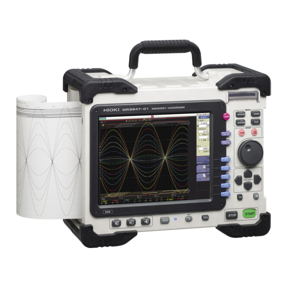
1.2 Names and Functions of Parts 1.2 Names and Functions of Parts Left Side Front Panel CF Card slot Handle Display (LCD) Printer Operating Keys ( p.11) Right Side USB Connector (Type B) Connect a USB cable here. p.278) External control terminals An external sampling signal can be USB Connector (Type A) - Page 21 1.2 Names and Functions of Parts Operating Keys STATUS DISP Displays the Status screen Displays the Waveform CHAN screen Displays the Channel screen SYSTEM FILE Displays the System screen Displays the File screen ( p.80) p.255) AB CSR CH.SET ...
-
Page 22: Screen Organization
1.3 Screen Organization 1.3 Screen Organization The screen configuration is as listed below. The display appears when a key is pressed. On the Waveform screen, the trigger settings window and channel settings window can be brought Waveform Screen This screen serves for observing the waveform. The settings window at the right shows the measurement parameters. - Page 23 1.3 Screen Organization Explanation of Screen Contents __________________________________ Waveform screen Title comment Trigger time Media icon Current date and time Shows the specified title Shows the date and time Shows the media status. Shows the date and time as set for ...
-
Page 24: Basic Key Operations
1.4 Basic Key Operations 1.4 Basic Key Operations Press the CURSOR key and move the cursor to the item on screen which you want to change. Check the GUI illustration and press the function key key) for the setting that you want to change. -
Page 25: Example For Using The Help Key
1.4 Basic Key Operations 1.4.1 Example for Using the HELP Key A simple explanation will appear at the cursor position. Help information can also be searched. Cursor Position Help Move the cursor to the item for which you want to display help. Press the HELP key. - Page 26 1.4 Basic Key Operations...
-
Page 27: Measurement Preparations
Measurement Chapter 2 Preparations Work Flow Install this instrument p.6) Install an input module p.18) (Adding or replacing an input module) Connect a logic probe to the Standard p.20) LOGIC terminals (When measuring logic signals) Connect the input cable(s) to the input ... -
Page 28: Install An Input Module
2.1 Install an input module 2.1 Install an input module Input modules specified at the time the instrument is ordered are supplied preinstalled. Use the fol- lowing procedures to add or replace input modules, or to remove them from the instrument. Preparations •... - Page 29 2.1 Install an input module If not installing another input module after removal Right Side Using the Phillips screwdriver, tighten the two mount- ing screws. Blank panel Measurements made without a blank panel installed may fail to meet specifications because of temperature instability within the instrument.
-
Page 30: Connecting Cords
2.2 Connecting Cords 2.2 Connecting Cords When measuring analog signals Connect the cables or sensors to the input module. When measuring logic signals Connect the logic probe(s) to the LOGIC terminal(s) on the instrument. When measuring power line voltage • The connection cords should only be connected to the secondary side of a breaker, so the breaker can prevent an accident if a short circuit occurs. - Page 31 2.2 Connecting Cords Measuring Voltage Applicable Input Modules Use to connect: Connection cords • 8966 Analog Unit • 8968 High Resolution Unit • 9197 Connection Cord • 8972 DC/RMS Unit (Maximum input voltage: 500 V) Large alligator clip type Connect to the BNC jack on an input mod- ule.
- Page 32 2.2 Connecting Cords Measuring frequency, number of rotations and Count Applicable Input Modules Use to connect: Connection cords • 8970 Freq Unit • 9197 Connection Cord (Maximum input voltage: 500 V) Connect to the BNC jack on an input mod- Large alligator clip type ule.
- Page 33 2.2 Connecting Cords Measuring Temperature Applicable Input Modules Use to connect: Thermocouple • 8967 Temp Unit (Compatible wire: AWG 16 to 26, 0.4 to 1.2 mm diameter) Connect to the terminal block on the input module. Connect to terminal block Insert to terminal block 25 mm Required item:...
- Page 34 Using a Strain Gauge to Measure Vibration or Displacement (Strain) Use to connect: Sensor Applicable Input Modules • 8969 Strain Unit • Strain Gauge Transducer (Not avail- able from Hioki) Connect Model 9769 Conversion Cable to • 9769 Conversion Cable the input module jack. Connecting using a 9769...
- Page 35 2.2 Connecting Cords Measuring Current Use to connect: Clamps Applicable Input Modules • 8971 Current Unit • Clamp-On Sensor 9272-10 Coneect Model 9318 Conversion Cable to • Universal Clamp-On CTs the input module jack. 9277, 9278, 9279 • AC/DC Current Sensors 9709, CT6862, CT6863 Example: 9272-10+9318...
- Page 36 2.2 Connecting Cords Measuring Logic Signals Use to connect: Logic Probe Applicable Input Modules • 8973 Logic Unit • 9320 Logic Probe LOGIC terminal • 9320-01 Logic Probe • MR9321 Logic Probe LA to LD are supplied as standard equip- •...
- Page 37 2.2 Connecting Cords Connect to LOGIC Terminals Example: Connecting the 9327 Logic Probe Right Side Required item: 9327 Logic Probe LOGIC terminals Connect the logic probe by aligning the groves on the plug and a LOGIC termi- nal. Connect to the measurement object. Connect to the measurement object...
-
Page 38: Recording Media Preparation
You may be unable to read from or save data to such cards. Hioki options PC cards (CF Card and adapter) 9726 PC Card 128M, 9727 PC Card 256M, 9728 PC Card 512M, 9729 PC Card 1G, 9830... - Page 39 Then pull the USB memory stick out. (No special steps are required at the instrument.) Depending on the intended use of the USB memory stick, connector types and settings at the instrument will differ, as listed in the table below. 8847 setting Connec- USB use Reference information...
-
Page 40: Formatting Storage Media
2.3 Recording Media Preparation 2.3.2 Formatting Storage Media Possible targets for formatting are CF Card, USB memory stick, hard disk, and internal memory. During the formatting process, a folder named "HIOKI8847" will be created. Note that formatting used storage media deletes all the information on the stor- age media and that deleted information is unrecoverable. -
Page 41: Loading Recording Paper
2.4 Loading Recording Paper 2.4 Loading Recording Paper The print head and surrounding metal parts can become hot. Be careful to avoid touching these parts. Be careful not to cut yourself with the paper cutter. • Please use only the specified recording paper. Using non-specified paper may not only result in faulty printing, but printing may become impossible. - Page 42 2.4 Loading Recording Paper Procedure Required item: 9231 Recording Paper, Paper roll axle (Supplied with the instrument) Press the Eject button to open the printer cover. Insert the paper roll axle into the paper roll core and mount the recording paper in the holder. Push the paper in until you hear a click.
-
Page 43: Supplying Power
Supplying Power 2.5.1 Connecting the Power Cord Connect the power cord to 8847 and plug it into an AC outlet. • When supplying power from an inverter or uninterruptible power supply (UPS), ensure that the following requirements are met. If the rated power supply voltage or frequency range is exceeded, or if a source with square wave output is used, the instrument may be fatally damaged and an electrical accident may occur. -
Page 44: Turning The Power On And Off
2.5 Supplying Power 2.5.3 Turning the Power On and Off This section explains the correct procedure for powering the unit up or down. Before turning the instrument on, make sure the supply voltage matches that indicated on the its power connector. Connection to an improper supply voltage may damage the instrument and present an electrical hazard. -
Page 45: Setting The Clocks
The instrument contains a built-in backup lithium battery, which offers a service life of about ten years. If the date and time deviate substantially when the instru- ment is switched on, it is the time to replace that battery. Contact your dealer or Hioki representative. -
Page 46: Adjusting The Zero Position (Zero-Adjust)
2.7 Adjusting the Zero Position (Zero-Adjust) 2.7 Adjusting the Zero Position (Zero-Adjust) This procedure compensates for input module differences and sets the reference potential of the instrument to 0 V. The compensation applies to the selected range. Before starting zero-adjust •... -
Page 47: Measurement Procedure
9790 Connection Cord 300 VAC/DC 300 VAC/DC 9197 Connection Cord 500 VAC/DC 600 VAC/DC L9198 Connection Cord 300 VAC/DC 600 VAC/DC 8847 Memory Input module Maximum rated HiCorder Maximum rated volt- input voltage age versus ground... -
Page 48: Measurement Workflow
3.2 Measurement Workflow 3.2 Measurement Workflow Pre-Measurement Inspection See: "3.3 Pre-Measurement Inspection" ( p.40) Make basic settings for measurement See: Select suitable recording method for "3.4.1 Measurement Function" ( p.41) measurement target "3.4.2 Time Axis Range and Sampling Rate" Set data acquisition speed ... - Page 49 3.2 Measurement Workflow Starting Measurement See: "3.6 Starting and Stopping Measurement" ( p.56) "Chapter 5 Saving/Loading Data & Managing Files" ( p.65) "Chapter 6 Printing" ( p.89) "7.1 Reading Measurement Values (Using the A/B Cursors)" ( p.102) ...
-
Page 50: Pre-Measurement Inspection
The following steps should be performed before measurement. Before using the instrument the first time, verify that it operates normally to ensure that the no damage occurred during storage or shipping. If you find any damage, contact your dealer or Hioki representative. -
Page 51: Setting Measurement Configuration
3.4 Setting Measurement Configuration 3.4 Setting Measurement Configuration Set measurement conditions as follows. By calling up the Waveform screen and then using the Settings window to make basic settings, you can immediately verify the effect of settings on the waveform. Basic settings can also be made by calling up the Status screen and selecting the [Status] sheet. - Page 52 3.4 Setting Measurement Configuration Description Recorder Function Values With the Recorder function, each data sample consists of the maximum and min- imum values acquired in the specified sampling period. So each data sample has its own amplitude breadth. Data of One Sample 1 2 3 4...
-
Page 53: Time Axis Range And Sampling Rate
3.4 Setting Measurement Configuration 3.4.2 Time Axis Range and Sampling Rate The timebase setting establishes the rate of input signal waveform acquisition, specified as time- per-division on the horizontal axis (time/div). The sampling setting specifies the interval from one sample to the next. (The setting is shown in brackets under the time axis range for the Memory function (see illustration at right). - Page 54 3.4 Setting Measurement Configuration Description Selecting the Refer to the table below when setting the time axis range. For example, to measure a 100 kHz waveform, the maximum display frequency set- time axis range ting range according to the table is 200 kHz - 800 kHz. If the maximum display fre- quency is set to 400 kHz, setting the time axis range to 10 μs/div is recommended.
- Page 55 3.4 Setting Measurement Configuration To automatically set the time axis range When you press the AUTO key, a suitable time range for the input sig- nal is selected and measurement starts. (This applies only to the Memory Function.) See: "3.7 Measurement With Automatic Range Setting (Auto-Ranging Func- ...
-
Page 56: Recording Length (Number Of Divisions)
3.4 Setting Measurement Configuration 3.4.3 Recording Length (number of divi- sions) Set the length (number of divisions) to record each time data is acquired. Procedure → To open the screen: Press the DISP Waveform screen Memory Function case Move the cursor to the [Shot] item. - Page 57 3.4 Setting Measurement Configuration Description Recording Length and Data Samples Each division of the recording length consists of 100 data samples. The total number of data samples for a specified recording length = set recording length (divisions) × 100 + 1. Recording Length and Number of Channels The available recording length is subject to limitations depending on the number of channels as selected from Status screen -...
-
Page 58: Screen Layout
3.4 Setting Measurement Configuration 3.4.4 Screen Layout You can specify the format in which the input signal is shown on the Waveform screen or printed out. Selecting X-Y1 screen or X-Y4 screen allows waveform X-Y synthesis. (This applies to the Memory function and X-Y recorder function.) ... -
Page 59: Input Channel Setting
3.5 Input Channel Setting 3.5 Input Channel Setting Set the analog channel and logic channel. Opening the Channel settings window See: "Displaying All Channels for Making the Variable Function Setting" ( p.135) Pressing [CH.SET] key repeat- edly displays the various sheets. [Analog] [Variable] [Logic]... -
Page 60: Channel Setting Workflow
3.5 Input Channel Setting 3.5.1 Channel Setting Workflow Explains the workflow to make settings for the analog channels (Ch1 - Ch16). Select the channels to use (Memory function) only) See: "8.4 Setting Channels to Use (Extending the Recording Length)" ( p.127) Make input and screen display related settings See:... - Page 61 3.5 Input Channel Setting • If the number of channels in use is low, not all channels may be selectable. • When input coupling is set to GND, the waveform will have no amplitude and range setting is not possible. •...
-
Page 62: Analog Channel
3.5 Input Channel Setting 3.5.2 Analog Channel Set the analog channel. For information on specific settings for 8967 Temp Unit, 8969 Strain Unit, and 8972 DC/RMS Unit, see "8.10"( p.140). Procedure → → → To open the screen: Press the DISP Waveform screen Press the... - Page 63 3.5 Input Channel Setting 4. Vertical axis Vertical axis (voltage axis) zoom-up or zoom-down settings can be made sepa- rately for each channel. The settings will be used for display and printout. (Voltage axis) Zooming is carried out using the zero position as reference. The measurement Zoom resolution does not change.
- Page 64 3.5 Input Channel Setting The zero position is as shown in the illustration below. (Example: 8966 Analog Unit) <Zoom factor ×1> Display screen Display screen Display screen (Zero position: 0%) (Zero position: 50%) (Zero position:100%) A/D Data 2047 100 % 2000 LSB 50 % A/D Data...
-
Page 65: Logic Channel
3.5 Input Channel Setting 3.5.3 Logic Channel Make settings for the logic channels. The channel settings window (Logic sheet) is shown when the display format is 1, 2, 4, or 8 screens. Procedure → → → To open the screen: Press the DISP Waveform screen Press the... -
Page 66: Starting And Stopping Measurement
3.6 Starting and Stopping Measurement 3.6 Starting and Stopping Measurement This section explains how to initiate and terminate a measurement. Procedure → To open the screen: Press the DISP Waveform screen Starting Measurement Press the START key to start measuring. •... - Page 67 3.6 Starting and Stopping Measurement Measurement and Internal Operations Measurement methods are normal measurement (start recording when measurement starts) and trigger measurement (start recording when trigger criteria START are satisfied).In this manual, "Measurement start" means the instant when you press the key, and "Recording start"...
-
Page 68: Measurement With Automatic Range Setting (Auto-Ranging Function)
3.7 Measurement With Automatic Range Setting (Auto-Ranging Function) 3.7 Measurement With Automatic Range Setting (Auto-Ranging Function) This applies only to the Memory function and analog modules. When you press the AUTO key after inputting a signal to an analog unit, and select [Auto Range], the horizontal axis (time axis) range, vertical axis (voltage... -
Page 69: X-Y Recorder Function
X-Y Recorder Chapter 4 Function • The X-Y waveform generated from the input signal is displayed in real time. • By saving the displayed data in memory, data can be stored as well as printed. • X-Similar to an X-Y pen recorder, waveform drawing can be controlled by simulated pen up/down operation. -
Page 70: Measurement Workflow
4.1 Measurement Workflow 4.1 Measurement Workflow Pre-Measurement Inspection See: "3.3 Pre-Measurement Inspection" ( p.40) Make basic settings for measurement See: Select X-Y recorder as measurement function "Function" ( p.61) Set sampling rate "Sampling" ( p.61) Determine screen layout format ... -
Page 71: Setting Measurement Configuration
4.2 Setting Measurement Configuration 4.2 Setting Measurement Configuration To set various measurement parameters, press the STATUS key to bring up the Status screen and select the [Status] sheet. (Settings for measurement function and sampling rate can also be made on the Waveform screen.) Description of setting items ______________________________________ Function Set the measurement function to X-Y recorder. -
Page 72: Starting And Stopping Measurement
4.3 Starting and Stopping Measurement 4.3 Starting and Stopping Measurement Press the DISP key to go to the Waveform screen. 1. Starting Measurement Press the START key to start measuring. 2. Pen Up/Down Operation Make this setting either during or before measurement. When the pen is set to Down, the waveform is being drawn. -
Page 73: Waveform Observation
4.4 Waveform Observation Redrawing with different waveform display settings • Also after clearing the waveform display, waveform data are still retained by the unit. This makes it possible to change settings for display format, display color, synthesis channels, channel zoom and offset before redrawing the waveform by selecting [Redraw]. - Page 74 4.4 Waveform Observation...
-
Page 75: Saving/Loading Data & Managing Files
Saving/Loading Data Chapter 5 & Managing Files Data can be saved and loaded and files can be managed. Before saving data, configure the save settings on the [File Save] sheet. Load data and manage files from the File screen. Opening the [File Save] sheet Pressing this key repeatedly... - Page 76 Opening the File screen The file order will be displayed. : Ascending order : Descending order Press this key. The selected file is indicated by a flashing cursor. Use the CURSOR keys to move between folder levels. Use the CURSOR keys to select a file.
-
Page 77: Data Capable Of Being Saved & Loaded
: File type cannot be handled by 8847. Files larger than 2 GB cannot be saved. Data Not Loadable on the Instrument ______________________________ • Data saved on devices other than the 8847 Memory HiCorder. • Image file ( • file... -
Page 78: Saving Data
5.2 Saving Data 5.2 Saving Data 5.2.1 Save Types and Workflow There are basically three types of save operations. To save data automatically To save data manually with the SAVE key ( p.74) during measurement Save data straight away Select data and save (... -
Page 79: Automatically Saving Waveforms
5.2 Saving Data 5.2.2 Automatically Saving Waveforms Measurement data are acquired for the recording length and then saved automatically each time. Save location and data type are selected before the measurement. Waveform data can be saved. Procedure → To open the screen: Press the SYSTEM [File Save] sheet... - Page 80 5.2 Saving Data Select the save area. Move the cursor to the [Save Area] item. Select Whole Save all recorded data. (default setting) Wave Save the data between the A and B cursors. If only the A cursor is Wave used, the range from the A cursor position to the end of the data is saved.
- Page 81 5.2 Saving Data Select the channel to save. Move the cursor to the [Save Channel] item. Select Disp Ch Saves the channels of all sheets for which waveform display is set to [On]. (default setting) All Ch Saves all measured channels (in the case of the memory function, channels has been set as [Used Ch] on the Status settings...
- Page 82 5.2 Saving Data Auto Save Operations __________________________________________ Example 1: Saving Files to the Topmost Directory of the Storage Media (A folder named "HIOKI8847" is created and file is saved there) 0000AUTO.MEM HIOKI8847 Save To: CF:\HIOKI8847 0001AUTO.MEM Save method: Normal Save File name will be "4-digit number Up to 5,000 files Folder to...
- Page 83 5.2 Saving Data Example 5: Saving data in an existing folder on the media using divided saving Save To: CF:\HIOKI8847\ HIOKI8847 0000AUTO.IDX TEST TEST 0000AUTO 0000AUTO.MEM Save method: Normal Save 0001AUTO.MEM Folder to 0001AUTO Folder name created au- save: Up to 5,000 files tomatically will be "4-digit number + folder name".
-
Page 84: Saving Data Selectively (Save Key)
5.2 Saving Data 5.2.3 Saving Data Selectively (SAVE Key) To use the SAVE key for quick saving, the saving conditions have to be set beforehand. The type of data to be saved are as following. (Settings data, waveform data, display screens, waveform screen, numerical calculation results) Procedure →... - Page 85 5.2 Saving Data Set the data to save. Move the cursor to the [Save Type] item. Select Save the settings data. Wave Save waveform data in binary format. Binary Select this to reload the waveform into the instrument. Wave Save waveform data in text format. Text Select this to use the waveform in a PC.
- Page 86 5.2 Saving Data Making advanced settings Available settings will differ, depending on the save type. Refer to the table below. Save Type Settings Description Setting Wave Division (Off, 16 M, 32 M) Binary Select this to divide a large file into several files for saving.
-
Page 87: Loading Data
5.3 Loading Data 5.3 Loading Data Data saved on media or in the internal memory of the instrument can be reloaded. Data Loading Workflow Before attempting to load data, make sure that the storage media is inserted and the loading target is correctly specified. - Page 88 Insert the storage media before making the media selection. Other limitations • Data saved with a Memory HiCorder model other than the 8847 cannot be loaded into the 8847. • When loading waveform data, the settings for the instrument are the same set- tings as when the data is saved.
-
Page 89: Automatically Loading Settings(Auto Setup Function)
5.4 Automatically Loading Settings (Auto Setup Function) 5.4 Automatically Loading Settings (Auto Setup Function) When settings are saved as described below, they can be loaded automatically at power-up. The Auto setup function is compatible with CF cards only. If the STARTUP file is on the HDD, USB memory stick, or RAM (internal mem- ory), it is not referenced. -
Page 90: Managing Files
5.5 Managing Files 5.5 Managing Files Press the key to display the File screen. Data saved to storage media can be managed on the FILE File screen. Use the keys to select a file from the file list. CURSOR Before performing an operation, insert the storage media (except for the optional hard disk). -
Page 91: Saving
PC. Data saved with this option cannot be loaded back into Specify the action if a file with the same name exists in the the 8847. To reload the data target folder. later into the 8847, use the "Binary" option. - Page 92 Saving divided data creates one or more waveform files and an index (IDX) file. Then by loading the IDX file, the data in the waveform file(s) is loaded as a batch. See: "Batch load of waveform data" ( p.78) Other limitations Text format data cannot be loaded into the 8847.
-
Page 93: Checking The Contents Of A Folder (Open A Folder)
5.5 Managing Files 5.5.2 Checking the Contents of a Folder (Open a Folder) See the contents of a selected folder (by opening that folder). Procedure → To open the screen: Press the FILE File screen To change the media: ( p.66) Move the cursor to the folder whose contents you want to see. -
Page 94: Deleting Files & Folders
5.5 Managing Files 5.5.4 Deleting Files & Folders Delete a file or folder. Procedure → To open the screen: Press the FILE File screen To change the media: ( p.66) Select the file or folder you want to delete. Select Select [Delete]. -
Page 95: Sorting Files
5.5 Managing Files 5.5.5 Sorting Files Sort files in the file list into a specified order. Procedure → To open the screen: Press the FILE File screen To change the media: ( p.66) Select [Sort], and select [Type] No sorting. Select Name Sorts files by file name characters. -
Page 96: Copying A File Into A Specified Folder
5.5 Managing Files 5.5.7 Copying a File Into a Specified Folder You can copy a file into a specified folder. Procedure → To open the screen: Press the FILE File screen To change the media: ( p.66) Move the cursor to the file you want to copy. Select Select [Copy]. -
Page 97: Printing The File List
5.5 Managing Files 5.5.8 Printing the File List The file list of the File screen can be printed. Details for all display items in the file list are printed. Only folder names are printed for folders. Information on the contents of folders is not printed. Before printing, make sure the recording paper is loaded correctly. - Page 98 5.5 Managing Files...
-
Page 99: Printing
Chapter 6 Printing [Printer] sheet lets you specify the print method and make other printing related settings. Opening the [Printer] sheet Pressing this key repeatedly displays the various sheets. [Environment] [Init] [File Save] [Printer] [Interface] Operations available from the [Printer] sheet Selecting the print method Making printer settings... -
Page 100: Printing Type And Workflow
6.1 Printing Type and Workflow 6.1 Printing Type and Workflow There are basically three types of printing operations. To print data in bulk after To print data automatically To selectively print data measurement by pressing during measurement after measurement PRINT Auto Print Selection Print Quick Print... -
Page 101: Making Auto Print Settings
6.2 Making Auto Print Settings Making Auto Print Settings This applies to the Memory function, Recorder function, and FFT function. Make these settings before measurement. Check to be sure that recording paper is loaded cor- rectly. Measurement data is printed automatically when you press the key to start measure- START ment. - Page 102 6.2 Making Auto Print Settings • When both Auto Print and Auto Save are enabled, Auto Save is executed first. • However, when the Roll Mode function (default setting: Auto) is used with the Memory function, Auto Print has priority. •...
-
Page 103: Manual Printing With Print Key (Selective Printing)
6.3 Manual Printing With PRINT key (Selective Printing) 6.3 Manual Printing With PRINT key (Selective Printing) Using the key from the Waveform screen, you can specify a range and data type for printing. PRINT This is also useful to prevent inadvertent printing due to operation errors. Procedure →... -
Page 104: Setting The Print Concentration Of The Waveform
6.4 Setting the Print Concentration of the Waveform 6.4 Setting the Print Concentration of the Wave- form The printing concentration of the waveform can be set for each channel. Procedure → To open the screen: Press the CHAN [Unit List] sheet, or [Each Ch] sheet... -
Page 105: Making Printer Settings
6.5 Making Printer Settings 6.5 Making Printer Settings Make settings on the [Printer] sheet of the System screen. Printer settings → To open the screen: Press the SYSTEM [Printer] sheet p.98) p.99) Select the print quality. Select Move the cursor to the [Print Speed] item. - Page 106 6.5 Making Printer Settings Printer settings → To open the screen: Press the SYSTEM [Printer] sheet p.98) p.99) Select the horizontal axis (time axis) display Select value. Time* Print the time from trigger event (unit is Move the cursor to the [Time Value] item.
- Page 107 6.5 Making Printer Settings Set the upper and lower limit value Select Move the cursor to the [Up/Low Print] item. Do not print upper and lower limits. (default setting) <Print Example> Print upper and lower limits. Upper and Lower Limit Set the zero-position comment Select Move the cursor to the...
-
Page 108: Miscellaneous Printing Functions
6.6 Miscellaneous Printing Functions 6.6 Miscellaneous Printing Functions You can produce a hard copy of the screen display, perform report printing or list printing. 6.6.1 Screen Hard Copy Press key while the screen to print is displayed. The printer will produce a hard copy of the COPY screen contents. -
Page 109: List Print
Create a text file using [Notepad] or another suitable application on the PC. The maximum size of the text comment that can be imported to the 8847 is 104 x 200. Print width will be adjusted to the widest line. Press the... - Page 110 6.6 Miscellaneous Printing Functions...
-
Page 111: Waveform Screen Monitoring And Analysis
Waveform Screen Monitoring Chapter 7 and Analysis Analytical operations such as display magnification, compression, and search are available on the Waveform screen. Opening the Waveform screen A cursor B cursor Scroll bar p.102) p.102) p.106) Upper Limit Value ... -
Page 112: Reading Measurement Values (Using The A/B Cursors)
7.1 Reading Measurement Values (Using the A/B Cursors) 7.1 Reading Measurement Values (Using the A/ B Cursors) • Time difference, frequency and potential difference (and when scaling is enabled, scaling values) can be read as numerical values using the A/B cursors on the Waveform screen. The cursors also allow specifying the calculation and print X-Y synthesis range. - Page 113 7.1 Reading Measurement Values (Using the A/B Cursors) Reading Measurement Values on Waveform Screen (for 1, 2, 4, 8 screens) → To open the screen: Press the DISP Waveform screen <Screen display (time axis cursor)> A Cursor B Cursor Values Between Cursor A Cursor B A/B cursors...
- Page 114 7.1 Reading Measurement Values (Using the A/B Cursors) Reading Measurement Values on Waveform Screen (for X-Y1, 4 screens) → To open the screen: Press the DISP Waveform screen <Screen display (X axis measurement value)> Cursor A Value X-Y synthesis of channel 1 and channel 2 waveform Channel A Cursor B Cursor...
-
Page 115: Specifying A Waveform Range (A/B Cursor)
7.2 Specifying a Waveform Range (A/B Cursor) 7.2 Specifying a Waveform Range (A/B Cursor) When the waveform is shown as a time display, the range can be specified with the div cursor or Trace cursor. The specified range will be used for file saving, printing, X-Y synthesis, and numerical calculation. The range selection will be retained also when the waveform display format is changed. -
Page 116: Moving The Waveform Display Position
7.3 Moving the Waveform Display Position Moving the Waveform Display Position This applies to the Memory function and Recorder function. 7.3.1 About Display Position From the scroll bar you can verify the relative position and size of the displayed portion of a wave- form within the overall recorded waveform. -
Page 117: Moving The Position (Jump Function)
7.3 Moving the Waveform Display Position 7.3.3 Moving the Position (Jump Function) You can specify the portion to be displayed immediately. Display location can be specified as follows: • Trigger point • A/B cursor location • Specified location (from the beginning [0%] to the end [100%]... -
Page 118: Performing Waveform X-Y Synthesis
7.4 Performing Waveform X-Y Synthesis Performing Waveform X-Y Synthesis This applies to the Memory function and X-Y recorder function. • To perform waveform X-Y synthesis, go to the Status screen, select the [Status] sheet, and set to X-Y1 screen or X-Y4 screen. By assigning any analog channel to the X axis and Y [Format] axis, up to 8 X-Y combo displays can be generated. - Page 119 7.4 Performing Waveform X-Y Synthesis Procedure → → → To open the screen: Press the DISP Waveform screen Press the CH.SET X-Y settings window Select Set the waveform color in the graph display. Waveform display is off. When a save channel Move the cursor to the for which you want to set the is specified as display channel, Auto Save will not be carried out.
-
Page 120: Magnifying And Compressing Waveforms
7.5 Magnifying and Compressing Waveforms Magnifying and Compressing Waveforms 7.5.1 Magnifying and Compressing Horizontal Axis (Time Axis) This applies to the Memory function and Recorder function. (However, with the Recorder function, waveform magnification is not available.) Data details can be observed by magnifying the waveform along the horizontal axis (time axis). Also, by compressing the time axis, overall waveform fluctuations can be readily seen. -
Page 121: Zoom Function (Magnifying A Section Of The Horizontal Axis (Time Axis)
7.5 Magnifying and Compressing Waveforms Zoom Function (Magnifying a Section 7.5.2 of the Horizontal Axis (Time Axis) This applies to the Memory function only. A magnified section of a waveform can be displayed together with the unmagnified view by splitting the screen horizontally. -
Page 122: Magnifying And Compressing Vertical Axis (Voltage Axis)
7.5 Magnifying and Compressing Waveforms To view the entire waveform (Memory function only) Move the cursor to the ratio item in the settings window and select [All Wave]. The waveform information for the entire recording length is displayed. Description About logic waveform display When the Zoom function is enabled, and the logic waveform display position is at less than [50pos], the logic waveform will not be displayed. -
Page 123: Monitoring Input Levels (Level Monitor)
7.6 Monitoring Input Levels (Level Monitor) 7.6 Monitoring Input Levels (Level Monitor) All input waveform levels can be monitored in real time. Analog channels and logic channels can be displayed at the same time. Procedure → the Menu To open : Press the DISP Display Menu... -
Page 124: Switching The Waveform Screen Display (Display Menu)
7.7 Switching the Waveform Screen Display (Display Menu) 7.7 Switching the Waveform Screen Display (Display Menu) The display menu allows you to bring up additional information such as upper/lower limit value indi- cation and comment display. It also allows you to set the waveform display width. ... -
Page 125: Seeing Block Waveforms
7.8 Seeing Block Waveforms 7.8 Seeing Block Waveforms This applies to the Memory function only. If recorded by memory division, the usage status of blocks can be checked. Furthermore, the desired block can be selected and the recorded waveform can be displayed. When memory division is not used, depending on the record length, it is possible to display the last 16 measured waveforms. - Page 126 7.8 Seeing Block Waveforms...
-
Page 127: Utility Functions
Chapter 8 Utility Functions Various utility functions are described in the section. Utility Functions Applicable measurements and settings Adding Comments ( p.118) • Displaying Waveforms During Recording Setting the channels to use p.124) (Making recording length longer) ( p.127) •... -
Page 128: Adding Comments
8.1 Adding Comments 8.1 Adding Comments This section explains how to enter title comments and channel comments. Information about alphanumeric input is also provided. 8.1.1 Adding a Title Comment When you enter a title comment, it can be displayed at the top of the Waveform screen, and it can also be printed. -
Page 129: Adding A Channel Comment
8.1 Adding Comments 8.1.2 Adding a Channel Comment Comments added for each channel can be displayed on-screen. Comments can also be printed on recording paper. (Allowed number of characters: up to 40) To copy a comment to another channel [Comment] sheet can be used to copy a comment. - Page 130 8.1 Adding Comments To select from preset terms Pressing the WAVE key after activating text input brings up a list of preset terms. It is also possible to select words from previously entered titles (History func- tion). See: "Entering Text From a Term List Or History List" ( p.122) Select the print content for each logic Select...
-
Page 131: Alphanumeric Input
8.1 Adding Comments 8.1.3 Alphanumeric Input Move the cursor to the setting item for which to make the input, and choose the content with the keys. Entering Text Move the cursor to the comment field and select [Enter Char]. A virtual keyboard appears. Select a character with the CURSOR key from the virtual keyboard, and select... - Page 132 8.1 Adding Comments Entering Text From a Term List Or History List While the virtual keyboard is displayed, pressing the WAVE key brings up a "Term List" and pressing the AB CSR key brings up a "History List". This can be used to enter preset terms or reuse text from a previous input session. Move the cursor to the comment field and select [Enter Char].
- Page 133 8.1 Adding Comments Entering Numerals By Up/Down Action Move the cursor to the numeric input field and select [Up-Down]. A virtual keyboard for digit input appears. Use the virtual keyboard to enter the numerals. (Use to move digit position, and use to increase or decrease the value.) Select...
-
Page 134: Displaying Waveforms During Recording (Roll Mode)
8.2 Displaying Waveforms During Recording (Roll Mode) 8.2 Displaying Waveforms During Recording (Roll Mode) This applies to the Memory function only. You can display and print the waveform at the same time as the data are acquired (if Auto Print is ... -
Page 135: Displaying New Waveforms Over Past Waveforms (Overlay)
8.3 Displaying New Waveforms Over Past Waveforms (Overlay) 8.3 Displaying New Waveforms Over Past Waveforms (Overlay) This applies to the Memory function only. Displayed waveforms are retained on-screen and overlaid with new waveforms. • Use this to compare new waveforms with those recorded immediately before. (When the trigger mode is [Repeat] or [Auto]) (... - Page 136 8.3 Displaying New Waveforms Over Past Waveforms (Overlay) Description When the Overlay function is enabled ([Auto] or [Manual]). • The Roll Mode function ( p.124) and Overlay functions ( p.125) cannot both be enabled at the same time. When the Roll Mode is enabled, the Over- lay function is automatically set [Off].
-
Page 137: Setting Channels To Use (Extending The Recording Length)
8.4 Setting Channels to Use (Extending the Recording Length) 8.4 Setting Channels to Use (Extending the Recording Length) This applies to the Memory function only. Select the analog and logic channels to use. Maximum recording length is available when the fewest necessary channels are enabled for use. Minimizing the number of channels in use allows memory to be reallocated to those channels being used. -
Page 138: Converting Input Values (Scaling Function)
8.5 Converting Input Values (Scaling Function) 8.5 Converting Input Values (Scaling Function) About the Scaling Use the scaling function to convert the measured voltage units output from a sensor Function to the physical units of the parameter being measurement. Hereafter, "scaling" refers to the process of numerical value conversion using the Scaling function. - Page 139 [Scale P2]. • When saving text or results of numerical calculation, some characters and symbols used for display on the instrument will be converted as follows. (8847 display → saved string) → ^2, → ^3 , μ → ~u, Ω→ ~o, ε→ ~e, °→ ~c , •...
-
Page 140: Scaling Setting Examples
8.5 Converting Input Values (Scaling Function) To reset Scaling settings: Move the cursor to the [Method], and select [Reset]. To copy the scaling setting to another channel The Channel screen - [Scaling] sheet can be used to copy a setting. ... - Page 141 8.5 Converting Input Values (Scaling Function) However, you may need to switch the vertical axis (voltage axis) range to suit actual input values. For example, to display ±0.2 V at full scale, set the vertical display to 20 mV per division (the instrument's 20 mV/div range) With scaling, signals from the sensor are acquired as current values.
- Page 142 8.5 Converting Input Values (Scaling Function) When a calibration factor is stated in the sensor's inspection records __ Set the [Method] item on the [Scaling] sheet to [Ratio]. Example 3 Measure using a sensor with a calibration factor of 0.001442 G / 1 x 10 strain , and display the measured data in [G] units.
- Page 143 8.5 Converting Input Values (Scaling Function) Using the dB value Example 5 Acquiring the conversion rate to convert 40 dB input to 60 dB 1. For scaling, set the [Method] to [Ratio]. 2. Point the cursor to the conversion rate setting. Select [dB Scaling] in the function column.
-
Page 144: Variable Function (Setting The Waveform Display Freely)
8.6 Variable Function (Setting the Waveform Display Freely) Variable Function (Setting the Waveform Dis- play Freely) The waveform height and display position can be arbitrarily set along the vertical axis (voltage axis) Precautions for using the Variable Function • Verify that the vertical axis (voltage axis) range is set properly for the input sig- nal. - Page 145 8.6 Variable Function (Setting the Waveform Display Freely) Make the Valiable Function Setting per channel _____________________ Procedure → To open the screen: Press the CHAN [Each Ch] sheet Enable the Variable function. Move the cursor to the [Variable], and select [On]. Set the display range per division Move the cursor to the [Range(div)], and enter numerical value.
- Page 146 8.6 Variable Function (Setting the Waveform Display Freely) Description When setting combined use of the Scaling and Variable functions When Auto-Correction of the Variable function is enabled (On, default set- ting) ( p.257) The Variable function settings change according to Scaling and vertical axis (voltage axis) range settings.
-
Page 147: Fine Adjustment Of Input Values (Vernier Function)
8.7 Fine Adjustment of Input Values (Vernier Function) 8.7 Fine Adjustment of Input Values (Vernier Function) Fine adjustment of input voltage can be performed arbitrarily on the Waveform screen. When recording physical values such as noise, temperature and acceleration using sensors, amplitude can be adjusted to facilitate calibration. -
Page 148: Inverting The Waveform (Invert Function)
8.8 Inverting the Waveform (Invert Function) 8.8 Inverting the Waveform (Invert Function) This applies to the analog channels only. You can invert the plus and minus sides of the waveform. Example: With a spring or similar, if pulling it towards the observer is taken as the minus direction and pushing it away from the observer as the plus direction, the output will be minus (negative) for pulling and plus (positive) for pushing. -
Page 149: Copying Settings To Other Channels (Calculation No.) (Copy Function)
8.9 Copying settings to other channels (calculation No.) (Copy function) 8.9 Copying settings to other channels (calcula- tion No.) (Copy function) At the following screens, settings can be copied to other channels and calculation No. (When the FFT function is used). •... -
Page 150: Making Detailed Settings For Input Modules
8.10 Making Detailed Settings for Input Modules 8.10 Making Detailed Settings for Input Modules Using the [Each Ch] sheet accessed from the Channel screen, you can make detailed settings. Opening the [Each Ch] sheet, Making a Channel Selection Shows the chan- nel number and channel position. -
Page 151: Making Settings For The Anti-Aliasing Filter (A.a.f.) (8968 High Resolution Unit)
8.10 Making Detailed Settings for Input Modules 8.10.1 Making Settings for the Anti-Aliasing Filter (A.A.F.) (8968 High Resolution Unit) See: Opening the [Each Ch] sheet, Making a Channel Selection ( p.140) A.A.F Enable the anti-aliasing filter to remove aliasing distortion. The cutoff frequency automatically changes according to the time axis range or (when the FFT function is used) the frequency range setting. -
Page 152: Settings For The 8967 Temp Unit
8.10 Making Detailed Settings for Input Modules 8.10.3 Settings for the 8967 Temp Unit See: Opening the [Each Ch] sheet, Making a Channel Selection ( p.140) Mode Set to match the type of thermocouple being used. Select Selections Measurement Range Selections Measurement Range Temp- K... - Page 153 8.10 Making Detailed Settings for Input Modules Renew Data The data refresh rate can be set to Fast, Normal, or Slow. (Data Refresh) The default setting is [Normal]. This allows stable measurement while removing noise. For quicker response, select [Fast], but note that this will make the mea- surement more susceptible to noise.
-
Page 154: Settings For The 8969 Strain Unit
8.10 Making Detailed Settings for Input Modules 8.10.4 Settings for the 8969 Strain Unit The 8969 Strain Unit can perform auto balance. When auto balance is performed, the reference output level of the conversion unit can be matched with the specified zero position. It is applicable only to a 8969 Strain Unit. -
Page 155: Settings For The 8970 Freq Unit
8.10 Making Detailed Settings for Input Modules 8.10.5 Settings for the 8970 Freq Unit When the display of standard logic channels (LA, LB, LC, and LD) is on, the 8970 Freq Unit installed on unit 1 or 2 can no longer be used. ... - Page 156 8.10 Making Detailed Settings for Input Modules Slope For each measurement mode, set the direction the specified level is exceeded. Select Selections Description ↑ Rises above the specified level are detected. (default setting) ↓ Drops below the specified level are detected. Devide Determines the frequency for each set pulse.
- Page 157 8.10 Making Detailed Settings for Input Modules Level This is enabled only when [Mode] [Pulse Width] or [Duty]. In pulse width/ duty rate measurements, set which level is detected when the threshold is exceeded. Select Selections Description High Measures above the threshold value. (default setting) Measures below the threshold value.
-
Page 158: Settings For The 8971 Current Unit
8.10 Making Detailed Settings for Input Modules 8.10.6 Settings for the 8971 Current Unit See: Opening the [Each Ch] sheet, Making a Channel Selection ( p.140) Mode There is no need to change the setting since it is set when the clamp sensor is automatically recognized. -
Page 159: Settings For The 8972 Dc/Rms Unit
8.10 Making Detailed Settings for Input Modules 8.10.7 Settings for the 8972 DC/RMS Unit See: Opening the [Each Ch] sheet, Making a Channel Selection ( p.140) Mode Switches between voltage measurement and RMS measurement. Select Selections Description Voltage measurement (default setting) RMS measurement Response Response can be set to three speeds: Fast, Normal and Slow. - Page 160 8.10 Making Detailed Settings for Input Modules...
-
Page 161: Chapter 9 Trigger Settings
Chapter 9 Trigger Settings Triggering is the process of controlling the start and stop of recording by specific signals or condi- tions (criteria). When recording is started or stopped by a specific signal, we say the trigger is "applied" or "triggering occurs". Trigger settings are made in the Trigger settings window of the Waveform screen. -
Page 162: Setting Workflow
9.1 Setting Workflow 9.1 Setting Workflow The procedure for making trigger settings is as follows. Trigger Mode Settings Set whether to continue to accept triggers after measuring. ( p.153) Make trigger source-related settings. Trigger Type Settings • Analog trigger p.154) ... -
Page 163: Setting The Trigger Mode
9.2 Setting the Trigger Mode 9.2 Setting the Trigger Mode Set whether to continue to accept triggers after measuring. If all trigger sources are disabled (Off, with no trigger setting), measurement starts immediately (free-running). Procedure key → Waveform screen To open the screen: Press the DISP Move the cursor to the [Trigger]... -
Page 164: Triggering By Analog Signals
9.3 Triggering by Analog Signals 9.3 Triggering by Analog Signals 9.3.1 Analog Trigger Settings and Types The steps for making settings and selecting the type of analog trigger are described below. The Trigger settings window ([Analog Trg.] sheet) is used. Procedure key →... - Page 165 9.3 Triggering by Analog Signals 1. Level Trigger ________________________________________________ A trigger is applied when an input signal crosses the specified trigger level (threshold voltage). Trigger Level Input Waveform ↑ ↓ Trigger Slope: In this manual, indicates a "trigger point", as the time at which a trigger is applied.
- Page 166 9.3 Triggering by Analog Signals Procedure key → Waveform screen → Press the key → Trigger settings To open the screen: Press the DISP TRIG.SET window ([Analog Trg.] sheet) 1. Level Trigger ( p.155) 2. In-Window Trigger Out-of-Window Trigger ( p.155) ...
- Page 167 9.3 Triggering by Analog Signals 4. In-Period Trigger, Out-of-Period Trigger __________________________ The rising edge and falling edge cycle of the reference voltage is measured, and triggering occurs when the cycle enters the preset range (In) or leaves the preset range (Out). ...
- Page 168 9.3 Triggering by Analog Signals When Using Noisy Signals for Triggering Method 1: Enable the trigger filter By setting the filter width to prevent triggering on noise, triggering occurs only when the trigger criteria continue to be met for at least the specified width (interval).
- Page 169 9.3 Triggering by Analog Signals Description About period range settings The period range settings for period triggering depend on the sampling period (sampling rate). (Changing the timebase also changes the period setting range.) The sampling rate setting can be verified on the Status screen - Status sheet. The upper threshold of the period range cannot be set below the lower threshold, and vice-versa.
-
Page 170: Triggering By Logic Signals (Logic Trigger)
9.4 Triggering by Logic Signals (Logic Trigger) 9.4 Triggering by Logic Signals (Logic Trigger) The steps for making settings and selecting the type of logic trigger are described below. The Trigger settings window ([Logic Trig] sheet) is used. • Input signals on logic channels serve as the trigger source. Triggering occurs when the specified trigger pattern and logical probe combining criteria (AND/ OR) are met. - Page 171 9.4 Triggering by Logic Signals (Logic Trigger) 3. Trigger Pattern Make the settings of the logic trigger pattern. Select Ignore signal. (default setting) Trigger at LOW signal level. Trigger at HIGH signal level. To copy the setting to another channel The Trigger settings window ([Logic Trig] sheet) can be used to copy a setting.
-
Page 172: Trigger By Timer Or Time Intervals (Timer Trigger)
9.5 Trigger by Timer or Time Intervals (Timer Trigger) 9.5 Trigger by Timer or Time Intervals (Timer Trigger) Set this to record at fixed times. • Triggering occurs at the specified interval from the specified Start time until the Stop time. •... - Page 173 9.5 Trigger by Timer or Time Intervals (Timer Trigger) Description About start and stop times • Start and Stop times should be set as times elapsed since the START key was pressed. • When the trigger mode is [Single] and the timer trigger is [On], only one timer trigger specified as the Start trigger is recognized.
- Page 174 9.5 Trigger by Timer or Time Intervals (Timer Trigger) When a trigger is applied from a trigger source other than a timer trigger Trigger sources set to On are all enabled. However, trigger timing depends on the trigger source settings. •...
-
Page 175: Applying An External Trigger (External Trigger)
9.6 Applying an External Trigger (External Trigger) 9.6 Applying an External Trigger (External Trig- ger) An external signal applied to the External Control terminal can serve as a trigger source. It can also be used to synchronously drive parallel triggering of multiple instruments. Procedure key →... -
Page 176: Pre-Trigger Settings
9.8 Pre-Trigger Settings 9.8 Pre-Trigger Settings This applies to the Memory function, and FFT function only. By setting a portion (number of divisions or percentage) of the recording length to occur before trig- gering, the waveform is recorded before as well as after the trigger point. You can also set the duration of a waveform to be recorded after a trigger point. - Page 177 9.8 Pre-Trigger Settings Description About pre-triggering and the recording period (recording length) Trigger Point Pre-Trigger setting examples 95% of the recording length is recorded before the trigger point 50% of the recording length is recorded before and 50% after the trigger point -95% 95% of the recording length is recorded after the trigger point •...
-
Page 178: Setting Trigger Acceptance (Trigger Priority)
9.8 Pre-Trigger Settings Setting Trigger Acceptance (Trigger 9.8.2 Priority) This applies to the Memory function only. You can set whether a trigger is recognized (accepted) if trigger criteria are met during this period. • When pre-triggering is enabled, trigger events are normally ignored for a cer- tain period after measurement starts (while recording the specified pre-trigger period). -
Page 179: Setting Trigger Timing
9.9 Setting Trigger Timing 9.9 Setting Trigger Timing This applies to the Memory function only. Set waveform recording operation when a trigger event occurs. Procedure key → Waveform screen → Press the key → Trigger settings window To open the screen: Press the DISP TRIG.SET Move the cursor to the... -
Page 180: Setting Combining Logic (And/Or) For Multiple Trigger Sources
9.10 Setting Combining Logic (AND/OR) for Multiple Trigger Sources 9.10 Setting Combining Logic (AND/OR) for Multiple Trigger Sources Analog, logic, external and timer trigger criteria can be combined by AND/OR logic to define com- plex trigger criteria. Procedure key → Waveform screen → Press the key →... -
Page 181: Using Trigger Settings To Search Measurement Data
9.11 Using trigger settings to search measurement data 9.11 Using trigger settings to search measure- ment data Trigger settings can be used to search measurement data. Locations that match the set trigger criteria in the measurement data are searched for and displayed sequentially. - Page 182 9.11 Using trigger settings to search measurement data Description Search results Locations that match the criteria are displayed in the center of the screen and an S mark is displayed in this position. When no matches are found, a message stating that no matches were found is dis- played.
-
Page 183: Numerical Calculation Functions
Numerical Calculation Chapter 10 Functions Numerical calculations can only be used with the Memory function. Results calculated from the acquired waveform are displayed as numerical values on the Waveform screen. Numerical calculation settings are made on the Status screen - [Num Calc] sheet. -
Page 184: Numerical Calculation Workflow
10.1 Numerical Calculation Workflow 10.1 Numerical Calculation Workflow There are two different ways of performing calculation. • Calculating While Measuring: Settings for numerical calculation must be made before the measurement. • Applying Calculations to Existing Data: Calculation is possible for waveform data after measurement is completed, and for data saved on media. - Page 185 10.1 Numerical Calculation Workflow Applying Calculations to Existing Data (Load the Data) (To load measurement data from storage media for calcu- p.77) lation) Make calculation settings on the Numerical Calculation p.176) Make Calculation Settings sheet ([Num Calc] sheet) ...
-
Page 186: Settings For Numerical Value Calculation
10.2 Settings for Numerical Value Calculation 10.2 Settings for Numerical Value Calculation Procedure → To open the screen: Press the STATUS [Num Calc] sheet Enable the Numerical Calculation function. Move the cursor to the [Numerical Calc] item. Select [On]. Specify the Numerical Calculation range. Move the cursor to the [Calc Area] item. - Page 187 10.2 Settings for Numerical Value Calculation When printing or saving calculation re- Select the channel for calculations. sults during measurement Move the cursor to the item for the calculation target, and Settings must be made before the mea- select the channel. surement.
- Page 188 10.2 Settings for Numerical Value Calculation Parameter table________________________________________________ Calculation Type Parameter Parameter description Period L (Level) Calculation is based on the interval (time) when this level is crossed. Frequency Only when the measurement signal has crossed the level and has not crossed the Pulse Width F (Filter) level again within the specified filter width, it is taken as a valid event.
-
Page 189: Displaying Numerical Calculation Results
10.2 Settings for Numerical Value Calculation 10.2.1 Displaying Numerical Calculation Results Numerical calculation results are displayed on the Waveform screen Calculation Results Press the DISP key. If the display is hard to view because of Numerical values and waveforms are displayed overlapping numerical values and wave- separately. -
Page 190: Judging Calculation Results
10.3 Judging Calculation Results 10.3 Judging Calculation Results Set the judgment criteria (upper and lower threshold values) by which to judge numerical calculation results. Judgment criteria can be set for every numerical calculation. Waveform acquisition processing depends on the trigger mode setting (Single or Repeat) and the criteria specified to stop measuring upon judgment (GO, NG or GO &... - Page 191 10.3 Judging Calculation Results Procedure → To open the screen: Press the STATUS [Num Calc] sheet Make calculation settings. ( p.176) Enable the judgment function. Lower limit Upper limit value value Move the cursor to the [Judge] setting for Calculation No. to judge, and select [On].
-
Page 192: Display Of Judgment Results And Signal Output
10.3 Judging Calculation Results 10.3.1 Display of Judgment Results and Signal Output Judgment results of numerical calculations are displayed on the Waveform screen. Within the judgment threshold range: GO judgment Out of the judgment threshold range: NG judgment (displayed in red) When printing, judgment results for each parameter are also printed. -
Page 193: Saving Numerical Calculation Results
10.4 Saving Numerical Calculation Results 10.4 Saving Numerical Calculation Results Calculate and automatically save during data acquisition. Before measurement begins, the calcula- tion settings need to be set. When using auto save during measurement, do not remove the storage media specified as the save destination until the measurement operation is completely finished. -
Page 194: Printing Numerical Calculation Results
10.5 Printing Numerical Calculation Results Example for saving numerical calculation results ___________________ If you save numerical calculation results, characters or display items used on the instrument are converted as shown below. Characters used on the instrument Saved characters μ Ω °... -
Page 195: Numerical Calculation Type And Description
10.6 Numerical Calculation Type and Description 10.6 Numerical Calculation Type and Description Numerical Calculation Description Type Obtains the average value of waveform data. AVE: Average value Average -- - n: Data count di: Data on channel number i Obtains the RMS value of waveform data. If Scaling is enabled, calculations are applied to the waveform after scaling. - Page 196 10.6 Numerical Calculation Type and Description Numerical Calculation Description Type The rise time of the acquired waveform from A% to B% (or fall time from B% to A%) is ob- tained by calculation using a histogram (fre- quency distribution) of the 0 and 100% levels of the acquired waveform.
- Page 197 10.6 Numerical Calculation Type and Description Numerical Calculation Description Type Finds the point where the signal crosses a speci- fied level from the start of the calculation range, Level Time to Level and obtains the time elapsed from the last trigger (Time-Lev) event.
- Page 198 10.6 Numerical Calculation Type and Description...
-
Page 199: Waveform Calculation Functions
Waveform Calculation Chapter 11 Functions Waveform calculations can only be used with the Memory function. A pre-specified calculation equation is applied to acquired waveform data, and the calculation results are displayed as a waveform on the Waveform screen. Waveform calculation settings are made on the Status screen - [Wave Calc] sheet. -
Page 200: Waveform Calculation Workflow
11.1 Waveform Calculation Workflow 11.1 Waveform Calculation Workflow There are two different ways of performing calculation. • Calculating While Measuring: Settings for waveform calculation must be made before the measurement. • Applying Calculations to Existing Data: Calculation is possible for waveform data after measurement is completed, and for data saved on media. - Page 201 11.1 Waveform Calculation Workflow Applying Calculations to Existing Data p.77) After measurement with calcula- (To load measurement data from storage media for calcu- tion OFF (Or with data loading) lation) p.192) Make Calculation Settings Make calculation settings on the Waveform Calculation sheet ([Wave Calc] sheet)
-
Page 202: Settings For Waveform Calculation
11.2 Settings for Waveform Calculation 11.2 Settings for Waveform Calculation Procedure → To open the screen: Press the STATUS [Wave Calc] sheet Enable the Waveform Calculation function. Move the cursor to the [Wave Calculation] item, and select [On]. Specify the waveform calculation range. Move the cursor to the [Calc Area] item. -
Page 203: Displaying The Waveform Calculation Results
11.2 Settings for Waveform Calculation [Confirm]. When finished entry, select The entered equation is displayed in the field. [Equation] The scale (maximum and minimum vales) of the calculation results has a default setting of [Auto]. If you want to scale the results, set the maximum and minimum values under [Manual]. - Page 204 11.2 Settings for Waveform Calculation About calculation equations _____________________________________ Operators Operator Name Operator Name Absolute Value DIF2 Derivative Exponent INT2 Integral Common Logarithm Sine Square Root Cosine Moving Average Tangent Movement parallel to the ASIN Inverse Sine time axis Derivative ACOS Inverse Cosine Integral...
-
Page 205: Setting Constants
11.2 Settings for Waveform Calculation 11.2.2 Setting constants Procedure → To open the screen: Press the STATUS [Wave Calc] sheet Move the cursor to the No. to be set as [CONST.]. Select an entry method, and enter the constant. Setting range: -9.9999E+29 to +9.9999E+29 ... -
Page 206: Changing The Display Method For Calculated Waveforms
11.2 Settings for Waveform Calculation 11.2.3 Changing the display method for calculated waveforms Procedure → To open the screen: Press the STATUS [Wave Calc] sheet Calculation No. To copy settings between Calculation Nos.: Select F1 [Copy]. Waveform Display Upper and Displayed Graph to display color... - Page 207 11.2 Settings for Waveform Calculation Waveform Calcu- Calculate the RMS waveform from the instantaneous waveform The RMS values of the waveform input on Channel 1 are calculated and dis- lation Example played. This example describes the calculation of waveform data measured for one cycle over two divisions.
-
Page 208: Waveform Calculation Operators And Results
11.3 Waveform Calculation Operators and Results 11.3 Waveform Calculation Operators and Results : ith member of calculation result data, d : ith member of source channel data Waveform Calculation Type Description Executes the corresponding arithmetic operation. Four Arithmetic Opera- tors ( +, -, *, / ) Absolute Value (ABS) = | d (i = 1, 2, .. - Page 209 11.3 Waveform Calculation Operators and Results : ith member of calculation result data, d : ith member of source channel data Waveform Calculation Type Description When d > 1, ≤ ≤ When -1 = acos(d Arccosine (ACOS) π When d <...
- Page 210 11.3 Waveform Calculation Operators and Results : ith member of calculation result data, d : ith member of source channel data Waveform Calculation Type Description First and second integrals are calculated using the trapezoidal rule. to d are the integrals calculated for sample times t to t Calculation formulas for the first integral Point t...
-
Page 211: Memory Division Function
Memory Division Chapter 12 Function Memory division function can only be used with the Memory function. Memory division settings are made on the Status screen - [Memory Div] sheet. p.115). Blocks to be displayed can also be selected on the Waveform screen Opening the [Memory Div] sheet... - Page 212 Operations available from the [Memory Div] sheet • Waveforms can be recorded into individual blocks by dividing memory space into multiple blocks. • You can record waveforms beginning at any block (Start Block), choose which blocks to display (Display Block), or display multiple overlaid blocks (Reference Block). •...
-
Page 213: Recording Settings
12.1 Recording Settings 12.1 Recording Settings Procedure → To open the screen: Press the STATUS [Memory Div] sheet Enable the Memory Division function. Move the cursor to the item. [Memory Div] Select [On]. Memory Division is disabled.(default setting) Memory Division is enabled. Set the number of divisions. -
Page 214: Display Settings
12.2 Display Settings 12.2 Display Settings Procedure → To open the screen: Press the STATUS [Memory Div] sheet To display any block on the Waveform screen Set the display blocks Set after measurement is complete.(This can also be set on the ... - Page 215 12.2 Display Settings Getting Details on Each Block: The trigger time and measurement status of each block can be viewed on the list. [Map/List] [List] Move the cursor to the , and select Block No. A block can be selected by the CURSOR keys or keys.
- Page 216 12.2 Display Settings Difference Between Dead Times During Normal and Memory Division Recording When both printer recording (Auto Print) and Auto Save are set for continuous triggering [Repeat] Anomalous phenomena occurring during dead times are not detected. Recording Dead Times Length Times during which sampling is inhibited due to internal processing, printing or saving When the Trace Waveform Display is disabled (Off) during Memory Division...
-
Page 217: Chapter 13 Fft Function
13.1 Overview and Features FFT Function Chapter 13 13.1 Overview and Features FFT analysis can only be used with the FFT function. The FFT (Fast-Fourier Transform) functions provide frequency analysis of input signal data. Use these functions for frequency analysis of rotating objects, vibrations, sounds and etc. ... -
Page 218: Operation Workflow
13.2 Operation Workflow 13.2 Operation Workflow Installation & Connections Turn Power On "Chapter 2 Measurement Preparations" ( p.17) Set the Function to FFT ( p.209) Settings Measure with New Settings Measure with Existing Settings [Status] sheet Set FFT analysis ( p.209) Set FFT analysis ( p.209) -
Page 219: Setting Fft Analysis Conditions
13.3 Setting FFT Analysis Conditions 13.3 Setting FFT Analysis Conditions Status screen [Status] sheet Basic measurement configuration settings are performed on the . Measure- p.225). ment configuration can be performed from the Waveform screen Opening the [Status] sheet Selecting the FFT Function 13.3.1 The FFT function can be selected at screens other than the file screen. -
Page 220: Selecting The Data Source For Analysis
13.3 Setting FFT Analysis Conditions 13.3.2 Selecting the Data Source for Analysis Select the data to be used for FFT analysis. There are two analysis methods: analysis using new measurements and analysis of data measured using the memory function. Procedure →... -
Page 221: Setting The Frequency Range And Number Of Analysis Points
13.3 Setting FFT Analysis Conditions 13.3.3 Setting the Frequency Range and Number of Analysis Points ___________________ About the frequency range and number of analysis points • The settings for the frequency range and number of analysis points determine the input signal acquisition time and frequency resolution. •... - Page 222 13.3 Setting FFT Analysis Conditions Relationship Between Frequency Range, Resolution and Number of Analysis Points Number of FFT Analysis Points Sampling Timebase 1,000 2,000 5,000 10,000 Range Sampling frequency [/div] [Hz] period Acquisi- Acquisi- Acquisi- Acquisi- [Hz] (MEM) Resolu- Resolu- Resolu- Resolu- tion...
-
Page 223: Thinning Out And Calculating Data
13.3 Setting FFT Analysis Conditions 13.3.4 Thinning Out and Calculating Data When performing FFT analysis of data measured using the memory function, the measurement data can be thinned before calculation. If the sampling frequency is too high and the expected results are not obtained, thin the data before calculation to increase the frequency resolution. -
Page 224: Setting The Window Function
13.3 Setting FFT Analysis Conditions 13.3.5 Setting the Window Function The window function defines the segment of the input signal to be analyzed. Use the window function to minimize leakage errors. There are three general types of window functions: • Hann window •... -
Page 225: Setting Peak Values Of Analysis Results
13.3 Setting FFT Analysis Conditions 13.3.6 Setting Peak Values of Analysis Results Either local or global maxima ([maximal]/ [maximum]) of the input signal and analysis results can be displayed on the Waveform screen. However, if Nyquist display is selected on the Status screen- [Status] sheet, no peak values are displayed. -
Page 226: Averaging Waveforms
13.3 Setting FFT Analysis Conditions 13.3.7 Averaging Waveforms The averaging function calculates the average of the values obtained from multiple measurements of a peri- odic waveform. This can reduce noise and other non-periodic signal components. Averaging can be applied to a time-domain waveform or to a spectrum. Procedure →... - Page 227 13.3 Setting FFT Analysis Conditions When averaging time-domain waveform values: Waveforms are acquired and averaged within the time domain. After averaging, FFT calculation is performed. When the trigger mode is [Auto]: Data is acquired when the START key is pressed, even if trigger criteria are not met after a certain interval.
- Page 228 13.3 Setting FFT Analysis Conditions Trigger Modes and Averaging If the trigger mode is [Single] or the calculation setting is [Once] Measurements continue until the specified number of averaging points is acquired. (Spectrum averaging) (Waveform averaging) Start Measurement Trigger analysis analysis START...
-
Page 229: Emphasizing Analysis Results (Phase Spectra Only)
13.3 Setting FFT Analysis Conditions 13.3.8 Emphasizing Analysis Results (phase spectra only) By specifying a setting factor (rate) to be applied to the input signal, the display of data exceeding the result- ing threshold can be emphasized. This feature is useful for viewing waveforms that may otherwise be obscured by noise. -
Page 230: Analysis Mode Settings
13.3 Setting FFT Analysis Conditions 13.3.9 Analysis Mode Settings Select the type of FFT analysis, channel(s), waveform display color and x and y axes. Procedure → To open the screen: Press the STATUS [Status] sheet See: To set from the Waveform screen ( p.225) Analysis Setting Contents... - Page 231 13.3 Setting FFT Analysis Conditions When [Parameter] setting contents are displayed Set the parameter. Move the cursor to the [Parameter] column of the Analysis No. to set. Select Analyze Parameter Setting Contents Filter: Normal nables the octave filter. 1/1 Octave, ...
- Page 232 13.3 Setting FFT Analysis Conditions Octave Filter Setting Filter features are based on JIS C1513-2002 class 1, class 2 (IEC61260). Sharp Normal Only those spectral component within the Filter characteristics approximate those octave band are used for analysis. Spec- of an analog filter.
- Page 233 13.3 Setting FFT Analysis Conditions Total harmonic distortion (THD) When the analysis mode is one of the following, the cursor appears and the distortion rate is calculated. (Linear spectrum, RMS spectrum, power spectrum) The distortion rate calculates the cursor position as the fundamental wave. When 2 cursors appear, the A cursor becomes the fundamental wave.
-
Page 234: 10Setting The Display Range Of The Vertical Axis (Scaling)
13.3 Setting FFT Analysis Conditions 13.3.10Setting the Display Range of the Vertical Axis (Scaling) The display range of the vertical (y) axis can be set to automatically suit analysis results, and can be freely expanded and compressed. Procedure → To open the screen: Press the STATUS [Status] sheet... -
Page 235: 11Setting And Changing Analysis Conditions On The Waveform Screen
13.3 Setting FFT Analysis Conditions 13.3.11Setting and Changing Analysis Conditions on the Waveform Screen The following settings can be made on the Waveform screen. Changes to the displayed analysis results become effective when the settings are changed. • Available settings are frequency range, number of analysis points, type of win- dow function, trigger mode and pre-triggering •... -
Page 236: Selecting Channels
13.4 Selecting Channels 13.4 Selecting Channels Channel selection is the same for all functions. For the setting method, refer to "3.5 Input Channel Setting" ( p.49) and "8.10 Making Detailed Settings for Input Modules" ( p.140). Scaling The scaling setting allows values displayed on this instrument to match the actual values read directly on a sound level meter or vibration meter. -
Page 237: Setting Screen Displays
13.5 Setting Screen Displays 13.5 Setting Screen Displays Set the display method for FFT calculation results. Procedure → To open the screen: Press the STATUS [Status] sheet Select the display format. Move the cursor to the [Format] item. Select the format of data to be displayed. The display format depends on the input data selected for analysis. - Page 238 13.5 Setting Screen Displays When “Drawing failed”: • NG: Nyquist, Running Spectrum The display format settings and analysis mode do not match. • NG: X-Axis Either change the [Format] setting and increase the number of screen divisions or change the display setting of the X-axis.
-
Page 239: Displaying Running Spectrums
13.5 Setting Screen Displays 13.5.1 Displaying running spectrums [Format] is set to [Running spectrum], changes in frequency over time can be observed. Procedure → To open the screen: Press the STATUS [Status] sheet Select the reference data. Move the cursor to the [Reference], and select [New Data]. - Page 240 13.5 Setting Screen Displays Procedure → To open the screen: Press the DISP Waveform screen Stopping waveform movement during measurement If the AUTO key is pressed during mea- surement, waveform movements can be stopped temporarily. The latest calculation results are displayed in the foreground.
- Page 241 13.5 Setting Screen Displays Changing the grid display The display format of the grid can be switched. Press the WAVE key on the panel of the unit. Move the cursor to the [Display]. Change the grid display Press F1 [Change Grid] key and change the grid display.
-
Page 242: Saving Analysis Results
13.6 Saving Analysis Results 13.6 Saving Analysis Results The saving procedure is the same as for the Memory and Recorder functions. See: "Chapter 5 Saving/Loading Data & Managing Files" ( p.65) The size of saved files depends on the save format and analysis method. ... -
Page 243: Printing Analysis Results
13.7 Printing Analysis Results 13.7 Printing Analysis Results The printing procedure is the same as for the Memory and Recorder functions. See: "Chapter 6 Printing" ( p.89) Example of Waveform Printout... -
Page 244: Analysis With The Waveform Screen
13.8 Analysis with the Waveform Screen 13.8 Analysis with the Waveform Screen 13.8.1 Analyzing after Specifying an Analysis Starting Point The FFT function can specify the calculation start position for waveforms measured by the memory function before calculation. Operation differs by calculation execution settings. ... - Page 245 13.8 Analysis with the Waveform Screen Specify the location of the analysis input data using the jog and shuttle controls. Moves the analysis starting point. Shuttle Memory Waveform Scrolls the Memory waveform. The analysis segment of the memory waveform for one pass is displayed. Select analysis conditions as occasion demands.
-
Page 246: Fft Analysis Modes
13.9 FFT Analysis Modes 13.9 FFT Analysis Modes 13.9.1 Analysis Modes and Display Examples For the functions of each analysis mode, see"13.9.2 Analysis Mode Functions" ( p.254). Storage Displays the time axis waveform of the input signal. When the window function setting is other than rectangular, the window function is applied to the waveform and displayed. - Page 247 13.9 FFT Analysis Modes Linear Spectrum The linear spectrum plots the input signal frequency. It can be displayed as a Nyquist plot. Main uses: • To inspect the peak frequency contents of a waveform • To inspect signal amplitudes at each frequency ...
- Page 248 13.9 FFT Analysis Modes Nyquist display • If the cursor is displayed, the total harmonic distortion (THD), which sets the fundamental wave as the cursor position, is displayed. When 2 cursors appear, the one with the low frequency becomes the fundamental. When results can- not be obtained, [---%] is displayed.
- Page 249 13.9 FFT Analysis Modes Normal display X axis: Log Y axis: Log-Mag Normal display X axis: Log Y axis: Lin-Real Normal display X axis: Log Lin-Imag Y axis: Lin-Imag If the cursor is displayed, the total harmonic distortion (THD), which sets the fun- damental wave as the cursor position, is displayed.
- Page 250 13.9 FFT Analysis Modes Power Spectrum Displays input signal power as the amplitude component. Main uses: • To inspect the peak frequency contents of a waveform • To inspect the power level at each frequency See: About the Functions"13.9.2 Analysis Mode Functions" ( p.254) Axis Display Type...
- Page 251 13.9 FFT Analysis Modes Power Spectrum Density Indicates the power spectrum density of the input signal with only the amplitude component included. This is the power spectrum divided by the frequency resolution. Main uses: To acquire a power spectrum with 1-Hz resolution for highly irregular waveforms such as white noise ...
- Page 252 13.9 FFT Analysis Modes LPC (Power Spectrum Density ) When the spectrum shape is complex and hard to comprehend with either linear or power spectra, a rough spectrum structure can be obtained.Main uses: To obtain a spectral envelope using statistical methods ...
- Page 253 13.9 FFT Analysis Modes Transfer Function From the input and output signals, the transfer function (frequency characteristic) of a measurement system can be obtained. It can also be displayed as a Nyquist plot. Main uses: • To inspect a filter’s frequency characteristic •...
- Page 254 13.9 FFT Analysis Modes Cross Power Spectrum The product of the spectra of two input signals can be obtained. The common frequency components of two signals can be obtained. Using the voltage and current waveforms as input signals, active power, reactive power and apparent power can be obtained at each frequency.
- Page 255 13.9 FFT Analysis Modes Impulse Response The transfer characteristic of a system is obtained as a time-domain waveform. Utilizing both output and input signals of the measurement system, a unit impulse is applied to the system and the corresponding response waveform is obtained. Main uses: To inspect circuit time constants ...
- Page 256 13.9 FFT Analysis Modes Coherence Function This function gives a measure of the correlation (coherence) between input and output signals. Val- ues obtained are between 0 and 1. Main uses: • To evaluate transfer functions • In a system with multiple inputs, to inspect the effect of each input on the output ...
- Page 257 13.9 FFT Analysis Modes Phase Spectrum Shows the phase characteristics of the input signal. Main uses: • To inspect the phase spectrum of channel 1. Displays the phase of a cosine waveform as a reference (0º). • To inspect the phase difference between channels 1 and 2. ...
- Page 258 13.9 FFT Analysis Modes Auto Correlation Function Shows the correlation of two points on the input signal at time differential t. Main uses: • To detect periodicy in irregular signals (improving and detecting SNR) • To inspect periodic components in a noisy waveform. ...
- Page 259 13.9 FFT Analysis Modes Cross-Correlation Function Using two input signals, shows the correlation of two points on the input signal at time differential t. Output is displayed as a function of differential time t. Main uses: • To determine the phase shift of two signals per unit of time •...
- Page 260 13.9 FFT Analysis Modes 1/1 Octave X axis: Log Y axis: Log-Mag Filter: Sharp 1/3 Octave X axis: Log Y axis: Log-Mag Filter: Normal 1/3 Octave X axis: Log Y axis: Log-Mag Filter: Sharp Not available with external sampling enabled. ...
- Page 261 13.9 FFT Analysis Modes Measurable Ranges with Octave Analysis...
- Page 262 13.9 FFT Analysis Modes...
- Page 263 13.9 FFT Analysis Modes...
-
Page 264: Analysis Mode Functions
13.9 FFT Analysis Modes 13.9.2 Analysis Mode Functions Analysis Mode Internal analysis formula (linear, real, imag [imaginary], log [logarithm]) No analysis. Storage Waveform A waveform obtained by applying the window function to a time-domain waveform. Histogram Counts amplitude data. Linear Spectrum RMS Spectrum Power Spectrum δ... -
Page 265: System Environment Settings
System Environment Chapter 14 Settings Use the System screen [Environment] sheet to make system-related settings. Opening the [Environment] sheet Pressing this key repeatedly displays the various sheets. [Environment] [Init] [File Save] [Printer] [Interface] See: "Chapter 16 External Control" ( p.287) - Page 266 Setting Descriptions____________________________________________ Grid Select the grid (graticule) type for the waveform screen. No grid displayed. Dotted Line Display a dotted-line grid. (default setting) Solid Line Display a solid-line grid. Time Value Display the time from the trigger point on the display. Time Display the time from the trigger point (fixed units).
- Page 267 Display Color Screen background and character colors on the Waveform screen can be set as desired. Select [Color Edit] change the (red), (green) and (blue) values p.258) of each item to change its color. Color 1 / Color 2 / Color 3 / Color Edit Beep Sound This function audibly indicates warnings and operating conditions by beep sounds.
- Page 268 Additional Description __________________________________________ Selecting a Select [Color Edit] to display the [Custom Color] screen. Screen Color Change the (red), (green) and (blue) values of each item to change its color. See: "8.1.3 Alphanumeric Input" ( p.121) [Custom Color] screen Color setting for each waveform Grid (graticule) color Colors of cursor A and B lines...
-
Page 269: Connection To A Computer
Connection to a Chapter 15 Computer This instrument is equipped with an Ethernet 100BASE-TX interface for LAN communications. You can control the instrument from PCs and other devices by connecting it to a network with 10BASE-T or 100BASE-TX cable (maximum length 100 m). It is also possible to directly connect the instrument to a computer via USB. -
Page 270: Lan Settings And Connection (Before Using Ftp/ Internet Browser/Command Communications)
15.1 LAN Settings and Connection (Before Using FTP/Internet Browser/Command Communications) 15.1 LAN Settings and Connection (Before Using FTP/ Internet Browser/Command Communications) The required settings are different, depending on whether the instrument is to be connected to an existing network or directly to a PC. Always make LAN settings before connecting to the network. -
Page 271: Setting Items
15.1 LAN Settings and Connection (Before Using FTP/Internet Browser/Command Communications) Setting Items Interface Select LAN or USB. Use DHCP* DHCP is a protocol that allows devices to automatically obtain and set their own IP addresses. *: Short for "Dynamic Host If you enable DHCP and there is a DHCP server operating in the same network, the Configuration Protocol"... - Page 272 15.1 LAN Settings and Connection (Before Using FTP/Internet Browser/Command Communications) LAN Setup Workflow Press the SYSTEM key and bring up the Communications sheet. According to the intended use, make set- tings as outlined below. Use the CURSOR keys to move the settings cursor, and use the keys to select a setting item.
-
Page 273: Connecting Instrument And Pc With Lan Cable
15.1 LAN Settings and Connection (Before Using FTP/Internet Browser/Command Communications) 15.1.2 Connecting Instrument and PC With LAN Cable Connect the instrument to a PC with a LAN cable as follows. Plug the LAN cable (100BASE-TX compliant) into the 100BASE-TX connector on the right side of the instrument. - Page 274 15.1 LAN Settings and Connection (Before Using FTP/Internet Browser/Command Communications) 2. Making 1:1 Connections Between the Instrument and a PC (Connecting the Instrument to a PC) You can monitor and control the instrument from a PC by connecting the instru- ment to the PC with LAN cable (100BASE-TX cable) Connection cable: Use one of the following.
-
Page 275: Performing Remote Operations On The Instrument (Use An Internet Browser)
15.2 Performing Remote Operations on the Instrument (Use an Internet Browser) 15.2 Performing Remote Operations on the Instrument (Use an Internet Browser) You can perform remote operations on the instrument from a PC by using an Internet browser. Attempting to control the instrument simultaneously from multiple computers may result in unintended operation. -
Page 276: Connecting To The Instrument With An Internet Browser
15.2 Performing Remote Operations on the Instrument (Use an Internet Browser) 15.2.2 Connecting to the Instrument With an Internet Browser The following example shows how to use the IE (Internet Explorer) browser on Windows XP. Launch IE on the PC and enter "http://" plus the IP address of the instrument in the address bar. If the IP address of the instrument is "192.168.0.2"... -
Page 277: Operating The Instrument With An Internet Browser
15.2 Performing Remote Operations on the Instrument (Use an Internet Browser) 15.2.3 Operating the Instrument With an Internet Browser Start/Stop Measurement You can start and stop a measurement. Measurement start/stop screen To open the screen: Click [Start/Stop] on list of operations. Procedure Click [Start]... -
Page 278: Remote Operation
15.2 Performing Remote Operations on the Instrument (Use an Internet Browser) Remote Operation The instrument can be controlled from a remote location. Remote Control Screen To open the screen: Click [Remote Control] on list of operations. The remote control screen is divided into the instrument display section and operation panel. Zoom in or out Operation panel Instrument display... - Page 279 15.2 Performing Remote Operations on the Instrument (Use an Internet Browser) Downloading Memory Data From Instrument You can download all data or data for a range specified by the A/B cursors. The data format can be binary, text, or Excel *: Microsoft Excel Memory Data Download Screen To open the screen: Click...
- Page 280 15.2 Performing Remote Operations on the Instrument (Use an Internet Browser) Downloading Data By FTP You can use FTP to download data from CF Card, HDD, or a USB memory stick. Data Download Screen for FTP To open the screen: Click [Acquire data by FTP] on list of operations.
- Page 281 15.2 Performing Remote Operations on the Instrument (Use an Internet Browser) Entering a Comment You can specify strings to be used as title comment, logic channel comment, and analog channel comment. Information about the module type and channel (installation location in the instrument) can be obtained and used only for the respective channel.
-
Page 282: Accessing The Files On The Instrument From A Computer (Using Ftp)
15.3 Accessing the Files on the Instrument From a Computer (Using FTP) 15.3 Accessing the Files on the Instrument From a Computer (Using FTP) By using a PC FTP client, you can transfer files from the instrument's media to the PC and perform other file operations. -
Page 283: Making Ftp Settings At The Instrument
15.3 Accessing the Files on the Instrument From a Computer (Using FTP) 15.3.1 Making FTP Settings at the Instrument Procedure → To open the screen: Press the SYSTEM [Interface] sheet Set the access restrictions. Move the cursor to the [Access Ctrl] item. -
Page 284: Using Ftp To Connect To The Instrument
You can also enter the user name and password, delimited by ':' and '@', in front of the normal IP address. [ftp:// Username:Password@ instrument IP address] Example: When the user name is "hioki" and the password is "1234": Enter [ftp://hioki:1234@192.168.0.2]. If the connection fails Check the communications settings of the instrument. -
Page 285: Using Ftp For File Operations
15.3 Accessing the Files on the Instrument From a Computer (Using FTP) 15.3.3 Using FTP for File Operations Downloading Files Select the file to download from the folder list and drag and drop* it on the down- load destination (the desktop or a folder outside the IE window). *: Click the file and hold the button down. -
Page 286: Transferring Data To The Pc
15.4 Transferring Data to the PC 15.4 Transferring Data to the PC The supplied USB Cable can be used to transfer data from the HDD to a PC. For information on how to use the supplied application software for data analysis, refer to the application's Help function. -
Page 287: Wave Viewer (Wv)
From the Windows Start button, open the [control panel] and click on [Add or remove programs]. Select [HIOKI Wave Viewer (Wv)] and uninstall the application. To upgrade to a newer version, uninstall the old version first and then install the new version. -
Page 288: Usb Settings And Connection (Before Command Communications)
15.6 USB Settings and Connection (Before Command Communications) 15.6 USB Settings and Connection (Before Com- mand Communications) Use the USB cable supplied with the instrument to connect the instrument to the PC. The instrument can then be controlled from the PC. Before command communication is possible, certain USB set- tings must be made and the connection must be established. - Page 289 15.6 USB Settings and Connection (Before Command Communications) After the "Found New Hardware" window appears, the [Found New Hardware Wizard] dialog box will appear. 8847 Memory HiCorder USB cable If after installing the driver you connect the instrument to the personal PC using a different USB port, the "Found New Hardware"...
- Page 290 (if there are check- marks next to any other items, uncheck them). Insert the included CD into the PC's CD-ROM derive and entering [X:/Driver/ 8847] in the location field. ([X] in the above file location indicates the CD-ROM drive. The letter allocated to the CD-ROM drive may vary by PC.)
- Page 291 15.6 USB Settings and Connection (Before Command Communications) Click [Continue Anyway]. After Windows XP checks the software, it will display a warning stating that the software has not been certified by Microsoft. Click [Continue Anyway]. Click Windows will begin copying the driver files. When installation is complete, the next dialog will appear.
-
Page 292: Controlling The Instrument With Command Communications (Lan/Usb)
15.7 Controlling the Instrument with Command Communications (LAN/USB) 15.7 Controlling the Instrument with Command Communications (LAN/USB) You can control the instrument remotely over the communications interface (LAN or USB). • For details, see the communications related documentation on the supplied application disc. -
Page 293: Making Settings On The Instrument
15.7 Controlling the Instrument with Command Communications (LAN/USB) 15.7.1 Making Settings on the Instrument Set items related to command communications. Procedure → To open the screen: Press the SYSTEM [Interface] sheet Select Set the delimiter. Send character code 0x0a. Move the cursor to the [Delimiter] item. -
Page 294: Communication Command Setting
15.7 Controlling the Instrument with Command Communications (LAN/USB) 15.7.2 Communication Command Setting The following example shows how to make a connection using the telnet software (HyperTerminal) supplied with Windows XP. Launch HyperTeminal. Click [Start], [Programs] [Accessories] [Com- munications] - [HyperTerminal], and then click [HyperTerminal]. - Page 295 15.7 Controlling the Instrument with Command Communications (LAN/USB) Make detailed connection settings. 1. Select [Properties] in the [File] menu. The Properties dialog for the specified connection name ap- pears. 2. Click the [Settings] tab. 3. Click the [ASCII Setup...] button. [ASCII Setup] dialog appears.
- Page 296 15.7 Controlling the Instrument with Command Communications (LAN/USB)
-
Page 297: Chapter 16 External Control
Chapter 16 External Control This chapter describes how to operate the instrument using the external control terminals. We use the term external control terminals generically to refer to all of the terminals. To avoid electrical hazards and damage to the instrument, do not apply voltage exceeding the rated maximum to the input terminals. -
Page 298: Connecting External Control Terminals
16.1 Connecting External Control Terminals 16.1 Connecting External Control Terminals The method for connecting to the external control terminals is as follows. Connecting External I/O Terminals (Connector Blocks) Cables to connect Recommended cables: single strand diameter: φ 1.0 mm (AWG18) 10 mm Single strand multi-strand: 0.75 mm... -
Page 299: External I/O
16.2 External I/O 16.2 External I/O 16.2.1 External Input (START/EXT.IN1) (STOP/EXT.IN2) (PRINT/EXT.IN3) External control signals can be applied to start and stop measurement, and to print and save data. The factory-default settings are to [Start], [Stop], and [Print]. Signal Input Procedure Connect the cables for the corresponding external input signals to START/ EXT.IN1, STOP/EXT.IN2, PRINT/EXT.IN3, and GND terminals. -
Page 300: External Output (Go/Ext.out1) (Ng/Ext.out2)
16.2 External I/O 16.2.2 External Output (GO/EXT.OUT1) (NG/EXT.OUT2) Signals can be output that indicate the instrument's judgment state. Signal Output Procedure Connect the GO/EXT.OUT1, NG/EXT.OUT2, and GND terminals to the device(s) to be controlled by single wires. See: "16.1 Connecting External Control Terminals" ( p.288) Press the SYSTEM... -
Page 301: External Sampling (Ext.smpl)
16.2 External I/O 16.2.3 External Sampling (EXT.SMPL) External sampling is possible only when the Memory Function is enabled. The sampling speed can be controlled by applying an external signal. Signal Input Procedure Connect the cables for the corresponding output signals to EXT.SMPL and GND terminals. -
Page 302: Trigger Output (Trig Out)
16.2 External I/O 16.2.4 Trigger Output (TRIG OUT) You can output a signal when a trigger event occurs. In addition, multiple instruments can be con- trolled for parallel synchronous operation. Signal Output Procedure Connect the cables for the output signals to TRIG OUT and GND terminals. ... -
Page 303: External Trigger Terminal (Ext.trig)
16.2 External I/O 16.2.5 External Trigger terminal (EXT.TRIG) You can input external signals as trigger sources. In addition, multiple instruments can be controlled for parallel synchronous operation. Signal Input Procedure Connect the cables for the corresponding external input signals to the EXT.TRIG and GND terminals. - Page 304 16.2 External I/O...
-
Page 305: Chapter 17 Specifications
17.1 General Specifications Chapter 17 Specifications 17.1 General Specifications Basic Specifications Measurement functions • Memory Function (high-speed data saving) • Recorder Function (real time recording) • X-Y Recorder Function • FFT Function No. of channels (max.) Analog 16 channels + Logic 16 channels (using the included logic probe input connector, ground is common with the GND terminal) or Analog 10 channels + Logic 64 channels (using supplied equipment plus up to three Model 8973 Logic Units) Memory capacity... -
Page 306: Display Section
17.1 General Specifications Display Section Display character Japanese/English Display type 10.4-in TFT Color LCD (800 × 600 dots) Display resolution T-Y waveform display: Normal 25 div (horizontal axis (time axis)) × 20 div (vertical axis (voltage axis)) X-Y waveform display: Normal 20 div (X axis) × 20 div (Y axis) Dot pitch 0.264 (Vertical) ×... - Page 307 17.1 General Specifications Waveform display magnifica- Horizontal axis (Time axis): ×10, ×5, ×2, ×1, ×1/2, ×1/5, ×1/10, ×1/20, ×1/50, ×1/100, ×1/200, tion ×1/500, ×1/1000, ×1/2000, ×1/5000, ×1/10000, ×1/20000 (expansion only with Memory function) Vertical axis (Voltage axis): ×100, ×50, ×20, ×10, ×5, ×2, ×1, ×1/2, ×1/5, ×1/10 Variable display function Included (Upper and lower display limits, or specified vertical divisions) Scaling...
-
Page 308: Measurement Specifications
17.2 Measurement Specifications 17.2 Measurement Specifications 17.2.1 Memory Function 5, 10, 20, 50, 100, 200, 500 μs/div Timebase 1, 2, 5, 10, 20, 50, 100, 200, 500 ms/div 1, 2, 5, 10, 30, 50, 100 s/div 1, 2, 5 min/div External sampling (100 S/div, adjustable settings) Time axis resolution 100 points/div... -
Page 309: X-Y Recording
17.2 Measurement Specifications 17.2.3 X-Y Recording Sampling period 1, 10, 100 ms Recording length Continuous Screen and Printing Settings X-Y 1 screen, X-Y 4 screens No. of X-Y display Up to 8 phenomena X-Y setting Select 8 channels out of 16 for X axis and Y axis Interpolation function Dot/Line (smooth trace) Waveform Clear... -
Page 310: Trigger Section
17.3 Trigger Section 17.3 Trigger Section Trigger method Digital comparison Trigger modes • Memory Function, FFT Function: Single, Repeat, or Automatic • Recorder Function: Single or Repeat Trigger source Analog Unit (Ch1 to Ch16), Standard Logic 16 Channels + Logic Unit (Max. 3 units, 48 Channels) External Trigger occurs by applying a 2.5 V falling edge signal, or shorted terminals Independent trigger criteria settable for each channel Free-run operation occurs when all trigger types are off. -
Page 311: File Specifications
17.4 File Specifications 17.4 File Specifications Data Saving Supported storage media CF Card, HDD, USB memory stick, Internal RAM Saved data Setting data, Measurement data, Analysis data, Screen image, Print image Saving types • Setting data (.SET) Setting configurations can only be saved to internal RAM •... -
Page 312: Built-In Functions
17.5 Built-In Functions 17.5 Built-In Functions Calculation-related functions Calculation functions Memory Function supported Number of calculations Up to 16 calculations can be applied to any channel Calculation range Whole range, or between A/B cursors Calculation types Average, RMS or P-P values, maximum, minimum and time to max/min values, period, frequency, rise time, fall time, standard deviation, squared value, X-Y squared value, time to level, level at time, pulse width, duty ratio, pulse count, four basic arithmetic operations, Time difference calcu- lation, phase contrast calculation, High level calculation, Low level calculation... - Page 313 17.5 Built-In Functions Position Display (VIEW) Functions Display function All types of positions, memory division blocks (only when using memory division), waveform search results, past waveform history (when memory division is OFF, depends on record length) Relative position display Displays the relative position of the currently displayed waveform within the overall recording length, and locations of cursors and trigger events Block display Block usage status (when memory division is ON) or past waveform history status (when memory...
-
Page 314: Input Modules Specifications
17.6 Input Modules Specifications 17.6 Input Modules Specifications 17.6.1 8966 Analog Unit Temperature and humidity range 23 ± 5°C (73 ± 9F°), 20 to 80% RH (when zero adjustment is executed 30 minutes after power on) for guaranteed accuracy Period of guaranteed accuracy 1 year No. -
Page 315: 8967 Temp Unit
17.6 Input Modules Specifications 17.6.2 8967 Temp Unit Temperature and humidity range 23 ± 5°C (73 ± 9F°), 20 to 80% RH (when zero adjustment is executed 30 minutes after power on) for guaranteed accuracy Period of guaranteed accuracy 1 year No. -
Page 316: 8968 High Resolution Unit
17.6 Input Modules Specifications 17.6.3 8968 High Resolution Unit Temperature and humidity range 23 ± 5°C (73 ± 9F°), 20 to 80% RH (when zero adjustment is executed 30 minutes after power on) for guaranteed accuracy Period of guaranteed accuracy 1 year No. -
Page 317: 8969 Strain Unit
17.6 Input Modules Specifications 17.6.4 8969 Strain Unit Temperature and humidity range 23 ± 5°C (73 ± 9F°), 20 to 80% RH (when auto balance is executed 30 minutes after power on) for guaranteed accuracy Period of guaranteed accuracy 1 year No. -
Page 318: 8970 Freq Unit
17.6 Input Modules Specifications 17.6.5 8970 Freq Unit Temperature and humidity range 23 ± 5°C (73 ± 9F°), 20 to 80% RH for guaranteed accuracy Measurement functions Based on voltage input, measures frequency, rotation speed, power frequency, integral values, pulse duty ratio, and pulse width. Connection terminal Insulated BNC terminal Input resistance... -
Page 319: 8971 Current Unit
For connecting the clamp sensor: Model 9318 Conversion Cable x 2, Instruction Manual Number of the 8971 available for Max. 4 unit (for Model 8847) Memory HiCoder *: During current measurement, add the accuracy and characeristic of clamp sensor using with Model 8971. -
Page 320: 8972 Dc/Rms Unit
17.6 Input Modules Specifications 17.6.7 8972 DC/RMS Unit Temperature and humidity range for 23 ± 5°C (73 ± 9F°), 20 to 80% RH (when zero adjustment is executed 30 minutes after power on) guaranteed accuracy Period of guaranteed accuracy 1 year No. -
Page 321: Maintenance And Service
The fuse is housed in the power unit of the instrument. If the power does not turn on, the fuse may be blown. If this occurs, a replacement or repair cannot be per- formed by customers. Please contact your dealer or Hioki representative. -
Page 322: Trouble Shooting
18.1 Trouble Shooting 18.1 Trouble Shooting If damage is suspected, check the "Troubleshooting" section before contacting your dealer or Hioki representative. If Power and Operating Keys Malfunction Symptom Check Item, or Cause Remedy and Reference display does Verify that the power cord is connected Is the power cord disconnected? properly. - Page 323 If Saving is Not Possible Symptom Check Item, or Cause Remedy and Reference "2.3 Recording Media Preparation" • Is your CF card Hioki certified? p.28) • Is the storage media inserted properly? • Is the storage media formatted? If saving is not possible to ...
-
Page 324: Initializing The Instrument
18.2 Initializing the Instrument 18.2 Initializing the Instrument 18.2.1 Initializing System Settings (System Reset) Select groups of settings currently in force on the instrument, and initialize the settings. Initialization returns the instrument to the factory default state. By default, the setting of [Setting (Stat, Ch, Trig)] and [Setting (Env)] are selected for initialization in this screen. -
Page 325: Error Messages
18.3 Error Messages 18.3 Error Messages A screen message appears whenever an error occurs. In either case, take the remedial action indicated. A beep may sound if the beeper setting on the [Environment] sheet is [Warn] [Warn+Action]. See: "Chapter 14 System Environment Settings" ( p.255) Warning Display Appears just once when an error... - Page 326 18.3 Error Messages Displayed Warnings Message Remedial Action Reference As other dialogs are displayed, selective sav- "5.2.3 Saving Data When executing, select "No" as the ing cannot be carried out. Either set the selec- Selectively (SAVE Key)" save property. tive saving during execution to [No] or close ...
- Page 327 18.3 Error Messages Displayed Warnings Message Remedial Action Reference "8.3 Displaying New Wave- The overlay function is not available when us- Cannot use.(Overlay) forms Over Past Waveforms ing the Roll mode. (Overlay)" ( p.125) "8.2 Displaying Waveforms Cannot use. (Overlay, Memory Division, If roll mode is used, these functions cannot be During Recording (Roll Wave Calculation)
-
Page 328: Self-Test (Self Diagnostics)
18.4 Self-Test (Self Diagnostics) 18.4 Self-Test (Self Diagnostics) The following self-test checks are available. Procedure → To open the screen: Press the SYSTEM [Init] sheet Check the instrument's internal memory (ROM and RAM). The results are displayed on the screen. ( p.318) ... -
Page 329: Printer Check
18.4 Self-Test (Self Diagnostics) Procedure (Common for Printer Check, Display Check, Key Check, System Configuration Check) → To open the screen: Press the SYSTEM [Init] sheet 18.4.2 Printer Check This check tests the condition of the printer. Before executing, check to be sure that recording paper is loaded. Things to check for after printer Move the cursor to the [Printer Check]... -
Page 330: System Configuration Check
18.4 Self-Test (Self Diagnostics) 18.4.5 System Configuration Check The list of installed options and other system information appears in a separate window. Move the cursor to the [System Information] item. Select [Exec]. The System Configuration List appears. To reappear the original screen: Press any key. -
Page 331: Cleaning
18.5 Cleaning 18.5 Cleaning Print Head Cleaning The print head and surrounding metal parts can become hot. Perform cleaning only after making sure that the parts have fully cooled down.Be careful to avoid touching these parts. Normally, no maintenance is required. However, depending on usage condi- tions, dirt and paper dust may accumulate on the thermal head over the long term, causing light or smeared printing. - Page 332 18.5 Cleaning About the Print Head Note the following precautions to avoid discoloring or deforming the instrument. • Do not use organic solvents such as thinner or benzene. • After washing, allow the printer to dry completely before use. About the Roller Surface •...
-
Page 333: Disposing Of The Instrument (Lithium Battery Removal)
18.6 Disposing of the Instrument (Lithium Battery Removal) 18.6 Disposing of the Instrument (Lithium Battery Removal) The instrument contains a lithium battery for memory backup. Remove this battery before disposing of the instrument. • To avoid electric shock, turn off the power switch and disconnect the power cord and connection cords before removing the lithium battery. - Page 334 18.6 Disposing of the Instrument (Lithium Battery Removal) Lithium Battery Removal Phillips screwdriver Slotted screwdriver Screw Upper side Handle cover Protector Front side Back side Remove Panel Back side Upper side Slide Lithium Battery Lead Circuit board...
-
Page 335: Appendix
Appendix 1 Default Values for Major Settings Appendix Appendix 1 Default Values for Major Settings Default values for major settings are listed below. Screen Sheet / Window Items Settings Timebase 5 μs/div Memory Recorder 10 ms/div Sampling (X-Y Recorder) 100 ms/S Shot 25 div Format... -
Page 336: Appendix 2 Reference
Appendix 2 Reference Appendix 2 Reference Appendix 2.1 Waveform File Sizes Refer to the following table for information about the waveform file sizes. References File Type Function Sizes Calculation method MEM File Memory Function p.A2) p.A4) REC File Recorder Function p.A2) - Page 337 Appendix 2 Reference FFT File Size (FFT Function) File size = header size + The size of the time axis data + the size of the mid-term data Calculation method:"FFT File" ( p.A4) Number of calculations Data Quantity 1,000 360KB 694KB 2,000...
- Page 338 Appendix 2 Reference Waveform File Size Calculation Method____________________________ MEM File File size (bytes) = setting size + data size *1: Setting size =23552 + 512 (analog channel portion + 4 x logic channel portion +Number of waveform calculation channels ) *2: Data size = 2 x (analog channel portion+logic channel portion + 2 xNumber of waveform calculation channels) x num- ber of data REC File...
-
Page 339: Appendix 2.2 Setting Configuration And Image Data File Sizes
Appendix 2 Reference Appendix 2.2 Setting Configuration and Image Data File Sizes For information on the size of setting and image data files, see the table below. File Size Setting file 33 KB BMP (No color compression) 470 KB BMP (Gray scale/No compression) 470 KB BMP (B/W/No compression) 59 KB... -
Page 340: Appendix 2.3 Timebase And Maximum Recordable Time
Appendix 2 Reference Appendix 2.3 Timebase and Maximum Recordable Time The maximum available recording time depends on the selected timebase. The maximum recording time can be obtained by the following formula. Recordable time can be verified on the Status Recordable Time = Timebase x Recording Length screen - [Status] sheet. - Page 341 Appendix 2 Reference Memory Function Channels used Timebase Sampling Maximum Recording Length (Time/div) Speed 16 channels 8 channels 4 channels 2 channels 40,000 div 80,000 div 160,000 div 320,000 div 5 μs 50 ns 200 ms 400 ms 800 ms 1.6 s 10 μs 100 ns...
-
Page 342: Appendix 2.4 Maximum Record Length And Number Of Divisions (Memory Division Function)
Appendix 2 Reference Appendix 2.4 Maximum record length and number of divisions (Memory division function) The maximum record length is automatically determined by settings for the number of channels used and the number of divisions. Desired record length Channels used The number of divisions 1-2 channels... -
Page 343: Appendix 2.5 Scaling Method When Using Strain Gauges
Appendix 2 Reference Appendix 2.5 Scaling Method When Using Strain Gauges This section describes how to determine the scaling conversion ratio when measuring with strain gauges and the Model 8969 Strain Unit. The appropriate conversion formula for stress depends on how the strain gauges are used. -
Page 344: Appendix 3 About Options
Items indicated "specify when ordering" are not user-installable. For new pur- chases, contact your supplier (agent) or nearest Hioki office. Input modules (Measurement amplifiers) These are installed by insertion into the compartments on the right side of the instrument. Modules can be swapped out as needed. - Page 345 Appendix 3 About Options (1),(2) 9277 Universal Clamp-On CT 20 A, DC to 100 kHz (1),(2) 9278 Universal Clamp-On CT 200 A, DC to 100 kHz AC/DC (1),(2) 9279 Universal Clamp-On CT* 500 A, DC to 20 kHz Following item (1) or (2) is (1),(2) 9709 AC/DC Current Sensor 500 A, DC to 100 kHz...
-
Page 346: Appendix 3.2 Model 9783 Carrying Case
• The case includes flammable materials, so do not place it near open flame or any object hotter than 100°C, as the case could catch fire. Parts Names 8847 Instrument Storage Compartment Manual Storage Compartment Option Storage Compartment Hinge Stopper... -
Page 347: Appendix 4 If The Model 9784 Dc Power Unit Is Installed
100 MΩ or more @ 500 V DC (between input and output, and between input and instrument chassis) Dimensions Adds approx. 29 mm (D) (1.14"D) to dimensions of Models 8847 Mass Adds approx. 1.20 kg (42.3 oz.) to the weight of Models 8847... - Page 348 Appendix 4 If the Model 9784 DC Power Unit is Installed • When using the DC Power Unit, printer specifications change as follows. 1. Maximum paper feed rate is 1 cm/s. (Consequently, real-time printing for continuous recording length operation is available at timebase settings slower than 1 s/div.) 2.
-
Page 349: Appendix 5 Fft Definitions
Appendix 5 FFT Definitions Appendix 5 FFT Definitions What is FFT? __________________________________________________ FFT is the abbreviation for Fast Fourier Transform, an efficient method to calcu- late the DFT (Discrete Fourier Transform) from a time-domain waveform. Also, the reverse process of transforming frequency data obtained by the FFT back into its original time-domain waveform is called the IFFT (Inverse FFT). - Page 350 Appendix 5 FFT Definitions Representing the above relationship on a complex flat surface produces the fol- lowing figure. Imaginary component φ 実数部 Real component Linear Time-Invariant Systems __________________________________ Consider a linear time-invariant (LTI) system y(n) that is a response to discrete time-domain signal (n).
- Page 351 Appendix 5 FFT Definitions Number of Analysis Points_______________________________________ The FFT functions of this instrument can perform frequency analysis of time- domain waveforms consisting of 1000, 2000, 5000, or 10,000 points. However, when the following conditions are satisfied, previously analyzed data can be reanalyzed with a different number of analysis points.
- Page 352 Appendix 5 FFT Definitions Aliasing ______________________________________________________ When the frequency of a signal to be measured is higher than the sampling rate, the observed frequency is lower than that of the actual signal, with certain fre- quency limitations. This phenomena occurs when sampling occurs at a lower fre- quency than that defined by the Nyquist-Shannon sampling theorem, and is called aliasing.
- Page 353 Appendix 5 FFT Definitions Anti-Aliasing Filters ____________________________________________ When the maximum frequency component of the input signal is higher than one- half of the sampling frequency, aliasing distortion occurs. To eliminate aliasing distortion, a low-pass filter can be used that cuts frequencies higher than one- half of the sampling frequency.
- Page 354 Appendix 5 FFT Definitions Imaging ______________________________________________________ When the instrument is set to a measurement frequency range that requires a higher sampling rate than the maximum capability of the input module, interme- diate data points are interpolated between successive data samples. In this case, the time-domain waveform exhibits a stair-step shape.
- Page 355 Appendix 5 FFT Definitions Averaging_____________________________________________________ With the FFT function, averaging is performed according to the following analyti- cal expressions. Averaging in the time domain produces meaningless data if per- formed with inconsistent trigger criteria. 1. Simple Averaging (Time and Frequency Domains) Sequences of acquired data are summed and divided by the number of acquisi- tions.
- Page 356 Appendix 5 FFT Definitions Window Function ______________________________________________ The Fourier transform of a continuous system is defined by the integral Calculus in expression (14) for the time range from minus infinity to plus infinity. ∞ π ε − (14) − ∞...
- Page 357 Appendix 5 FFT Definitions The following figure presents an example of spectral analysis by applying a win- dow function to a time-domain waveform. Using the window function, discontinuous points on the time-domain waveform are eliminated, so the wave shape approaches a line spectrum. When a Blackman-Harris window function is applied to a time-domain waveform (...
- Page 358 Appendix 5 FFT Definitions Exponential window 0.1% 0.1% 99.9% 99.9% Frequency (1/W) Time-Domain Waveform Spectrum Hamming window Frequency (1/W) Time-Domain Waveform Spectrum Blackman window Frequency (1/W) Time-Domain Waveform Spectrum Blackman-Harris window Frequency (1/W) Time-Domain Waveform Spectrum...
- Page 359 Appendix 5 FFT Definitions Flat top window Frequency (1/W) Time-Domain Waveform Spectrum The following example shows input sine waves of 1050 and 1150 Hz analyzed with different window functions. Because the frequencies in this example are close to one another, a rectangular window with a narrow main lobe is able to separate and display both frequencies, but a Hann window with a wide main lobe displays the two as a single spectral component.
- Page 360 Appendix 5 FFT Definitions Octave Filter Characteristics _____________________________________ Octave filter characteristics are determined according to IEC61260 standards. The figures below show these standards and the filter characteristics of this instrument. 1/1 Octave Filter Characteristic Gain [dB] Gain [dB] Normal filter ノ...
- Page 361 Appendix 5 FFT Definitions Linear Predictive Coding (LPC) ___________________________________ In the following figure, linear predictive coding is implemented by passing a sam- ple of the input signal through the prediction filter while altering the filter so as to minimize errors in the original signal. Input Signal Error Signal 入力信号...
- Page 362 Appendix 5 FFT Definitions...
-
Page 363: Index
Index Index Index Numerics Communications ..........259 Access ............273 Command Communications ......282 100BASE-TX .............263 Delimiter ........... 283 2-Point ...............129 Header ............. 283 8969 Strain Unit ..........144 Command Port (Port number) ...... 282 9769 Conversion cable ......24, 27 Deleting and Renaming Files ....... - Page 364 Index Index Hanning Window ..........214 Hard Disk (HDD) ..........29 Entering Numerals ........... 123 Help ..............15 Entering Text ............ 121 HELP Key ............15 ESC key ............. 11 High Level ............187 Event Count ............. 158 Highlight ............219 Exponential ............
- Page 365 Index Index Power spectrum density ........241 POWER Switch ..........34 Magnifying and Compressing ......110 Pre-Trigger ............166 Zoom Function ..........111 Pre-trigger ............166 Manual Trigger ..........165 Print ..............89 Maximal .............215 Auto print ............90 Comments ............ 118 Maximam ............215 Data to save ...........
- Page 366 Index Index Using a Clamp-On Probe ......130 Time to Maximum Value (Max-Time) ....185 Using a strain gauge ........132 Time to Minimum Value (Min-Time) ....185 Using Model 8969 Strain Unit ...... 131 Timebase ............212 Using strain gauges ........
- Page 367 Index Index Waveform Calculations Settings ............192 Waveform Color ..........196 Waveform color ..........225 Waveform File Sizes .......... A2 Waveform Screen ..........234 Window Compensation ..........214 Window Function ..........214 Window function ....... 214, 225, A22 Window trigger ..........155 X Axis ..............221 X-Y Area ...........176, 186 Y Axis ..............221...
- Page 368 Index Index...
- Page 372 HIOKI USA CORPORATION 6 Corporate Drive, Cranbury, NJ 08512, USA TEL +1-609-409-9109 FAX +1-609-409-9108 Edited and published by Hioki E.E. Corporation Technical Support Section • All reasonable care has been taken in the production of this manual, but if you find any points which are unclear or in error, please contact your supplier or the International Sales and Marketing Department at Hioki headquarters.
Need help?
Do you have a question about the 8847 and is the answer not in the manual?
Questions and answers