Texas Instruments TI-92 Getting Started
Hide thumbs
Also See for TI-92:
- Installing instruction (7 pages) ,
- Replacing instructions (5 pages) ,
- Manual (7 pages)
Advertisement
Quick Links
C H A P T E R
5
T
I
TI-92
EXAS
NSTRUMENTS
5.1 Getting Started with the TI-92
In this book, the key with the green diamond symbol inside a green border will be indicated by
, the key with the
white arrow pointing up inside a white border (the shift key) will be indicated by
, and the key with the white
arrow (the backspace key) pointing to the left will be indicated by
. Although the cursor pad allows for
movements in eight directions, we will mainly use the four directions of up, down, right, and left. These directions
will be indicated by
,
,
, and
, respectively
There are eight blue keys on the left side of the calculator labeled F1 through F8. These function keys have different
effects depending on the screen that is currently showing. The effect or menu of the function keys corresponding to
a screen are shown across the top of the display.
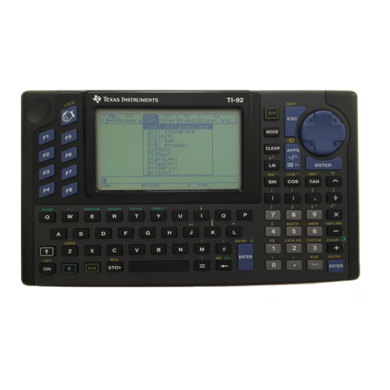
5.1.1 Basics: Press the ON key to begin using your TI-92. If you need to adjust the display contrast, first press
,
then press – (the minus key) to lighten or + (the plus key) to darken. To lighten or darken the screen more, press
then + or – again. When you have finished with the calculator, turn it off to conserve battery power by pressing 2nd
and then OFF. Note that the TI-92 has three ENTER keys and two 2nd keys which can be used interchangeably.
Check your TI-92's settings by pressing MODE. If necessary, use the cursor pad to move the blinking cursor to a
setting you want to change You can also use F1 to go to page 1 or F2 to go to page 2 of the MODE menu. To
change a setting, use
to get to the setting that you want to change, then press
to see the options available. Use
or
to highlight the setting that you want and press ENTER to select the setting. To start with, select the options
shown in Figures 5.1 and 5.2: function graphs, main folder, floating decimals with 10 digits displayed, radian
measure, normal exponential format, real numbers, rectangular vectors, pretty print, full screen display, Home
screen showing, and approximate calculation mode. Note that some of the lines on page 2 of the MODE menu are
not readable. These lines pertain to options that are not set as above. Details on alternative options will be given later
in this guide. For now, leave the MODE menu by pressing
HOME or 2nd QUIT. Some of the current settings are
shown on the status line of the Home screen.
Figure 5.1: MODE menu, page 1
Figure 5.2: MODE menu, page 2
Copyright © Houghton Mifflin Company. All rights reserved.
Advertisement

Related Manuals for Texas Instruments TI-92


Summary of Contents for Texas Instruments TI-92
- Page 1 5.1.1 Basics: Press the ON key to begin using your TI-92. If you need to adjust the display contrast, first press then press – (the minus key) to lighten or + (the plus key) to darken. To lighten or darken the screen more, press then + or –...
- Page 2 HOME, or APPS ENTER. Figure 5.3: APPS menu 5.1.2 Editing: One advantage of the TI-92 is that you can use the cursor pad to scroll in order to see a long calculation. For example, type this sum (Figure 5.4): 1 + 2 + 3 + 4 + 5 + 6 + 7 + 8 + 9 + 10 + 11 + 12 + 13 + 14 + 15 + 16 + 17 + 18 + 19 + 20 Then press ENTER to see the answer.
- Page 3 To edit a previous expression that is no longer on the entry line, press 2nd and then ENTRY to recall the prior expression. Now you can change it. In fact, the TI-92 retains as many entries as the current history area holds in a “last entry”...
- Page 4 5.1.3 Key Functions: Most keys on the TI-92 offer access to more than one function, just as the keys on a computer keyboard can produce more than one letter (“g” and “G”) or even quite different characters (“5” and “%”). The primary function of a key is indicated on the key itself, and you access that function by a simple press on the key.
- Page 5 Figure 5.7: ANS variable 5.1.7 The MATH Menu: Operators and functions associated with a scientific calculator are available either immediately from the keys of the TI-92 or by the 2nd keys. You have direct access to common arithmetic –1 , ∧), trigonometric functions (SIN, COS, TAN), and their inverses (2nd SIN...
- Page 6 2nd MATH 7[Probability] 1[!] ENTER. On the TI-92 it is possible to do calculations with complex numbers. To enter the imaginary number i, press 2nd i. For example, to divide 2 + 3i by 4 – 2i, press ( 2 + 3 2nd i ) ÷ (4 – 2 2nd i ) ENTER. The result is 0.1 + 0.8i (Figure 5.9).
- Page 7 Home screen, with cSolve( on the entry line. To complete the computation, press X ∧ 3 – 4 X ∧ 2 + 14 X – 20 = 0 , X) ENTER. The TI-92 will display the real and complex roots of the equation, as shown in Figure 5.10.
- Page 8 Figure 5.14: Table of values 5.2.2 Functions in a Graph Window: Once you have entered a function in the Y= screen of the TI-92, just press GRAPH to see its graph. The ability to draw a graph contributes substantially to our ability to solve problems.
- Page 9 + 4x extends infinitely far left and right and also infinitely far up and down, the TI-92 can display only a piece of the actual graph. This displayed rectangular part is called a viewing rectangle. You can easily change the viewing rectangle to enhance your investigation of a graph.
- Page 10 Enter a new value to over-write a previous value and then press ENTER. Remember that a minimum must be less than the corresponding maximum or the TI-92 will issue an error message. Also, remember to use the (-) key, not –...
- Page 11 5.2.3 Graphing Step and Piecewise-Defined Functions: The greatest integer function, written [[x]] , gives the greatest integer less than or equal to a number x. On the TI-92, the greatest integer function is called floor( and is located under the Number sub-menu of the MATH menu (Figure 5.8). From the Home screen, calculate [[6.78]] = 6 by pressing 2nd MATH 6[floor(] 6.78) ENTER.
- Page 12 Figure 5.29 shows this graph in a viewing rectangle from –5 to 5 in both directions. This was done in Dot style, since the TI-92 will (incorrectly) connect the two sides of the graph at x = 0 if the function is graphed in Line style.
- Page 13 Figure 5.34: A “square” circle horizontal The two semicircles in Figure 5.34 do not meet because of an idiosyncrasy in the way the TI-92 plots a graph. 5.2.5 TRACE: Graph the function y = –x + 4x from Section 5.2.2 using the standard viewing rectangle. (Remember to clear any other functions in the Y= screen.) Press any of the cursor directions...
- Page 14 Graphing Technology Guide: TI-92 Press F3[TRACE] to enable the left and right directions to move the cursor along the function. The cursor is no longer free-moving, but is now constrained to the function. The coordinates that are displayed belong to points on the function’s graph, so the y-coordinate is the calculated value of the function at the corresponding x-coordinate.
- Page 15 Check the WINDOW screen to see that the xmin and xmax are automatically updated. The TI-92 has a display of 239 horizontal columns of pixels and 103 vertical rows, so when you trace a curve across a graph window, you are actually moving from xmin to xmax in 238 equal jumps, each called ∆x. You would −...
- Page 16 Figure 5.48: After a zoom in As you see in the F2[Zoom] menu (Figure 5.43), the TI-92 can zoom in (press F2[Zoom] 2) or zoom out (press F2[Zoom] 3). Zoom out to see a larger view of the graph, centered at the cursor position. You can change the horizontal and vertical scale of the magnification by pressing F2[Zoom] C[SetFactors] (see Figure 5.49) and...
- Page 17 FACTORS menu and go back to the graph. (Pressing 2nd QUIT will take you back to the Home screen.) Technology Tip: The TI-92 remembers the window it displayed before a zoom. So if you should zoom in too much and lose the curve, press F2[Zoom] B[Memory] 1[ZoomPrev] to go back to the window before. If you want to execute a series of zooms but then return to a particular window, press F2[Zoom] B[Memory] 2[ZoomSto] to store the current window’s dimensions.
- Page 18 Then the accuracy of your approximation will be such that the error is less than the distance between two tick marks. Change the x-scale on the TI-92 from the WINDOW menu. Move the cursor down to xscl and enter an appropriate value.
- Page 19 – 36x + 17 in a window large enough to exhibit all its x-intercepts, corresponding to all the equation’s zeros (roots). Then use trace and zoom, or the TI-92’s zero finder, to locate each one. In fact, this equation has just one solution, approximately x = –1.414.
- Page 20 The TI-92 has a solve( function. To use this function, you must be in the Home screen. To use the solve( function, press S O L V E ( 24 X ∧ 3 – 35 X + 17 = 0 , X) ENTER. The TI-92 displays the value of the zero (Figure 5.59).
- Page 21 TI-92 will prompt for the function that you want to have the shading above. Use to move the cursor to the graph of x – 4, then press ENTER. The TI-92 will then prompt for the function that you want to have the shading −...
- Page 22 ENTER The first line of keystrokes sets the TI-92 in degree mode and calculates the sine of 45 degrees. While the calculator is still in degree mode, the second line of keystrokes calculates the sine of π degrees, approximately 3.1415°. The third line changes to radian mode just before calculating the sine of π...
-
Page 23: Scatter Plots
(as noted in Section 5.1.3) can affect the outcome of calculations. In the previous example, the degree sign must be inside of the parentheses so that when the TI-92 is in radian mode, it calculates the tangent of 45 degrees, rather than converting the tangent of 45 radians into an equivalent number of degrees. - Page 24 Graphing Technology Guide: TI-92 and press F1 [Manage] 1 [Delete] ENTER. The TI-92 will ask you to confirm the deletion by pressing ENTER once more. Now press APPS 6[Data/Matrix Editor] 3[New] P R I Z E ENTER to open a new variable called PRIZE (Figure 5.66).
- Page 25 Data/Matrix Editor, press F5[Calc]. For the Calculation Type, choose 5[LinReg] and set the x variable to c1 and the y variable to c2. In order to have the TI-92 graph the regression equation, set Store RegEQ to as y1(x) as shown in Figure 5.70.
- Page 26 Remember to clear or deselect the plot before viewing graphs of other functions. 5.6 Matrices 5.6.1 Making a Matrix: The TI-92 can work with as many different matrices as the memory will hold. Here’s how − ...
- Page 27 multiplication of c by a, press C × A ENTER. If you tried to multiply a by c, your TI-92 would notify you of an error because the dimensions of the two matrices do not permit multiplication in this way.
- Page 28 RowAdd(expression, matrix1, Index1, Index2). Note that your TI-92 does not store a matrix obtained as the result of any row operation. So, when you need to perform several row operations in succession, it is a good idea to store the result of each one in a temporary place.
- Page 29 Thus z = 2, so y = –1, and x = 1. Technology Tip: The TI-92 can produce a row-echelon form and the reduced row-echelon form of a matrix. The row-echelon form of matrix a is obtained by pressing 2nd MATH 4[Matrix] 3[ref(] A) ENTER and the reduced row-echelon form is obtained by pressing 2nd MATH 4[Matrix] 4[rref(] A) ENTER.
- Page 30 Continue to use each answer as n in the next calculation. Here are keystrokes to accomplish this iteration on the TI-92 calculator. (See the results in Figure 5.84.) Notice that when you use ANS in place of n in a formula, it is sufficient to press ENTER to continue an iteration.
- Page 31 Y= to edit any of the TI-92’s sequences, u1 through u99. Make u1(n) = u1(n – 1) + 4 and u1(1) = 7 by pressing U 1 ( N – 1) + 4 ENTER 7 ENTER (Figure 5.85). Press 2nd QUIT to return to the Home screen. To find the 18th term of this sequence, calculate u1(18) by pressing U 1 ( 18 ) ENTER (Figure 5.86).
- Page 32 5.8 Parametric and Polar Graphs 5.8.1 Graphing Parametric Equations: The TI-92 plots parametric equations as easily as it plots functions. Up to ninety nine pairs of parametric equations can be plotted. In the first page of the MODE menu (Figure 5.1) change the Graph setting to PARAMETRIC.
- Page 33 Figure 5.92: Polar to rectangular coordinates 5.8.3 Graphing Polar Equations: The TI-92 graphs polar functions in the form r = f (θ) . In the Graph line of the MODE menu, select POLAR for polar graphs. You may now graph up to ninety nine polar functions at a time. Be sure that the angle measure has been set to whichever you need, RADIAN or DEGREE.
- Page 34 Graphing Technology Guide: TI-92 Figure 5.93 shows rectangular coordinates of the cursor’s location on the graph. You may sometimes wish to trace along the curve and see polar coordinates of the cursor’s location. The first line of the Graph Format menu (Figure 5.24) has options for displaying the cursor’s position in rectangular (RECT) or polar (POLAR) form.
- Page 35 In the program, each line begins with a colon : supplied automatically by the calculator. Any command you could enter directly in the TI-92’s Home screen can be entered as a line in a program. There are also special programming commands.
- Page 36 Graphing Technology Guide: TI-92 : (–b + (d) )/(2a) → m ( (-) B + 2nd D) ) ÷ ( 2 A) STO➧ M ENTER calculates one root and stores it as m : (–b – (d))/(2a) → n ( (-) B – 2nd D) ) ÷...
- Page 37 If you need to interrupt a program during execution, press ON. After the program has run, the TI-92 will display the appropriate message and the root(s). The TI-92 will be on the Program I/O screen not the Home screen. The F5 key toggles between the Home screen and the Program I/O screen or you can use 2nd QUIT, HOME to go to the Home screen, or the APPS menu to go any screen.
- Page 38 ∆ → a good approximation to the limit. Figure 5.97: Using nDeriv( The TI-92 has a function , nDeriv(, which is available in the Calculus sub-menu of the MATH menu, that will + ∆ − − ∆ calculate the symmetric difference, .
- Page 39 The | is found on the keyboard above the K, so press 2nd K to enter it. If no value for ∆x is provided, the TI-92 automatically uses ∆x = 0.001. If no value for x is given, the TI- 92 will give the symmetric difference as a function of x.
- Page 40 Press ENTER repeatedly until two successive approximations differ by less than some predetermined value, say 0.0001. Note that each time you press ENTER, the TI-92 will use the current value of x, and that value is changing as you continue the iteration.
- Page 41 5.12.2 Areas: You may approximate the area under the graph of a function y = f (x) between x = A and x = B with your TI-92. To do this you use the F5[Math] menu when you have a graph displayed. For example, here are the keystrokes for finding the area under the graph of the function y = cos x between x = 0 and x = 1.